Downloaded 707 times
![• comma or space separated values between brackets
»row = [1 2 5.4 -6.6]
»row = [1, 2, 5.4, -6.6];
• Command window:
• Workspace:
Row Vector:](https://image.slidesharecdn.com/matlab-150220160218-conversion-gate01/75/MATLAB-Programming-26-2048.jpg)
![• Semicolon separated values between brackets
»column = [4;2;7;4]
• Command window:
• Workspace:
Column vector:](https://image.slidesharecdn.com/matlab-150220160218-conversion-gate01/75/MATLAB-Programming-27-2048.jpg)
![• Make matrices like vectors
• Element by element
» a= [1 2;3 4];
• By concatenating vectors or matrices (dimension matters)
Matrix:](https://image.slidesharecdn.com/matlab-150220160218-conversion-gate01/75/MATLAB-Programming-30-2048.jpg)
![• ones:
>> x = ones(1,7) % All elements are ones
• zeros:
>> x = zeros(1,7) % All elements are zeros
• eye:
>> Y = eye(3) % Create identity matrix 3X3
• diag:
>> x = diag([1 2 3 4],-1) % diagonal matrix with main
diagonal shift(-1)](https://image.slidesharecdn.com/matlab-150220160218-conversion-gate01/75/MATLAB-Programming-31-2048.jpg)
![• magic:
>> Y = magic(3) %magic square matrix 3X3
• rand:
>> z = rand(1,4) % generate random numbers
from the period [0,1] in a vector 1x4
• randint:
>> x = randint(2,3, [5,7]) % generate random integer
numbers from (5-7) in a matrix 2x3](https://image.slidesharecdn.com/matlab-150220160218-conversion-gate01/75/MATLAB-Programming-32-2048.jpg)
![• Addition and subtraction are element-wise ‛ sizes must match‛:
• All the functions that work on scalars also work on vectors
»t = [1 2 3];
»f = exp(t);
is the same as
»f = [exp(1) exp(2) exp(3)];](https://image.slidesharecdn.com/matlab-150220160218-conversion-gate01/75/MATLAB-Programming-34-2048.jpg)
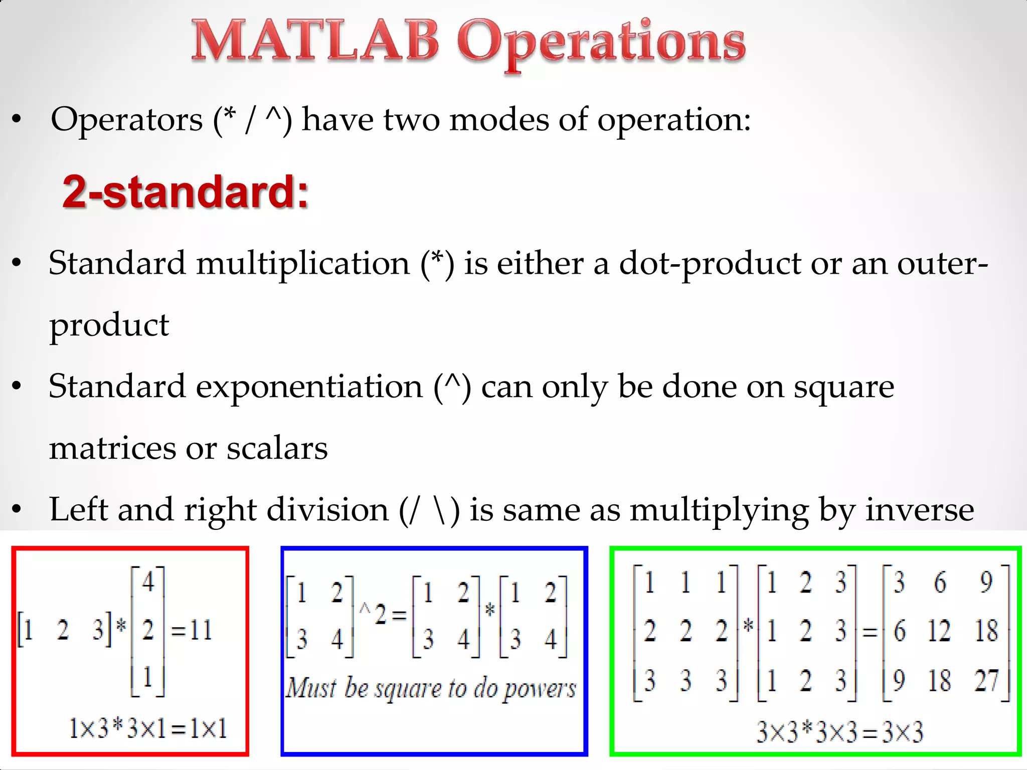
![• Operators (* / ^) have two modes of operation:
1-element-wise :
• Use the dot: .(.*, ./, .^). ‚BOTH dimensions must match.‛
»a=[1 2 3]; b=[4;2;1];
»a.*b, a./b, a.^b all errors
»a.*b', a./b’, a.^(b’) all valid](https://image.slidesharecdn.com/matlab-150220160218-conversion-gate01/75/MATLAB-Programming-35-2048.jpg)
![o min(x); max(x) % minimum; maximum elements
o sum(x); prod(x) % summation ; multiplication of all elements
o length(x); % return the length of the vector
o size(x) % return no. of row and no. of columns
o anyVector(end) % return the last element in the vector
o find(x==value) % get the indices
o [v,e]=eig(x) % eign vectors and eign values
Exercise:
>>x = [ 16 3 2 13 ; 5 10 11 8 ; 9 6 7 12 ; 4 15 14 1 ]](https://image.slidesharecdn.com/matlab-150220160218-conversion-gate01/75/MATLAB-Programming-37-2048.jpg)
![o fliplr(x) % flip the vector left-right
o Z=X*Y % vectorial multiplication
o y= sin(x).*exp(-0.3*x) % element by element multiplication
o mean %Average or mean value of every column.
o transpose(A) or A’ % matrix Transpose
o sum((sum(A))')
o diag(A) % diagonal of matrix
Exercise:
>>x = [ 16 3 2 13 ; 5 10 11 8 ; 9 6 7 12 ; 4 15 14 1 ]](https://image.slidesharecdn.com/matlab-150220160218-conversion-gate01/75/MATLAB-Programming-38-2048.jpg)
![• To get the minimum value and its index:
»[minVal , minInd] = min(vec);
maxworks the same way
• To find any the indices of specific values or ranges
»ind = find(vec == 9);
»[ind_R,ind_C] = find(vec == 9);
»ind = find(vec > 2 & vec < 6);
Indexing:](https://image.slidesharecdn.com/matlab-150220160218-conversion-gate01/75/MATLAB-Programming-43-2048.jpg)
![>> X =[ 16 3 2 13 ; 5 10 11 8 ; 9 6 7 12 ; 4 15 14 1 ]
>>X(:,2) = [] % delete the second column of X
X =
16 2 13
5 11 8
9 7 12
4 14 1
Deleting Rows & Columns:](https://image.slidesharecdn.com/matlab-150220160218-conversion-gate01/75/MATLAB-Programming-44-2048.jpg)
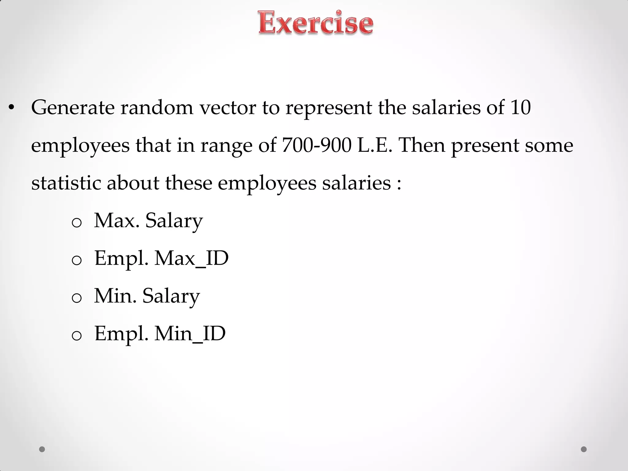
![• Generate random vector to represent the salaries of 10
employees that in range of 700-900 L.E.
clear;
clc;
close all;
Salaries =randint(1,10,[700,900]);
MaxSalary = max(Salaries); % Max. Salary
EmplMax_ID = find(Salaries==MaxSalary); %Empl. Max_ID
MinSalary = min(Salaries); %Min. Salary
EmplMin_ID = find(Salaries==MinSalary); %Empl. Min_ID](https://image.slidesharecdn.com/matlab-150220160218-conversion-gate01/75/MATLAB-Programming-49-2048.jpg)

![Plot surface in the 3D :
x = linspace(1,10,20);
y = linspace(1,5,10);
[XX,YY] = meshgrid(x,y);
ZZ = sin(XX)./exp(YY);
mesh(ZZ)
0
2
4
6
8
10
12
14
16
18
20
0
2
4
6
8
10
-0.4
-0.3
-0.2
-0.1
0
0.1
0.2
0.3
0.4](https://image.slidesharecdn.com/matlab-150220160218-conversion-gate01/75/MATLAB-Programming-62-2048.jpg)
![Specialized Plotting Functions:
polar : to make polar plots
»polar(0:0.01:2*pi,cos((0:0.01:2*pi)*2))
•bar : to make bar graphs
»bar(1:10,rand(1,10));
•stairs : plot piecewise constant functions
»stairs(1:10,rand(1,10));
•fill : draws and fills a polygon with specified vertices
»fill([0 1 0.5],[0 0 1],'r');](https://image.slidesharecdn.com/matlab-150220160218-conversion-gate01/75/MATLAB-Programming-63-2048.jpg)
![Axes Control:
• For tow-dimensional graphs:
>>axis([xmin xmax ymin ymax])
• For three-dimensional graphs:
>>axis([xmin xmax ymin ymax zmin zmax])
• To reenable MATLAB automatic limit selection:
>>axis auto
• makes the x-axis and y-axis the same length:
>>axis square](https://image.slidesharecdn.com/matlab-150220160218-conversion-gate01/75/MATLAB-Programming-64-2048.jpg)
![Cell Array:
• Used to store different data type (classes) like vectors, matrices,
strings,<etc in single variable.
• Variables declaration:
>> X=3
>> Y=[1 2 3;4 5 6]
>> Z(2,5)=15
>> A(4,6)=[3 4 5] %…..(wrong)
• cell array:
>> C{1}=[2 3 5 10 20]
>> C{2}=‘hello’
>> C{3}=eye(3)
1 0 0
0 1 0
0 0 1
C
2 3 5 10 20 h e l l o](https://image.slidesharecdn.com/matlab-150220160218-conversion-gate01/75/MATLAB-Programming-90-2048.jpg)
![Cell Array:
Z{2,5} = linspace(0,1,10)
Z{1,3} = randint(5,5,[0 100])
Z{1,3}(4,2) =77
Note:
• The default for cell array elements is empty
• The default for matrix elements is zero
77
Z](https://image.slidesharecdn.com/matlab-150220160218-conversion-gate01/75/MATLAB-Programming-91-2048.jpg)
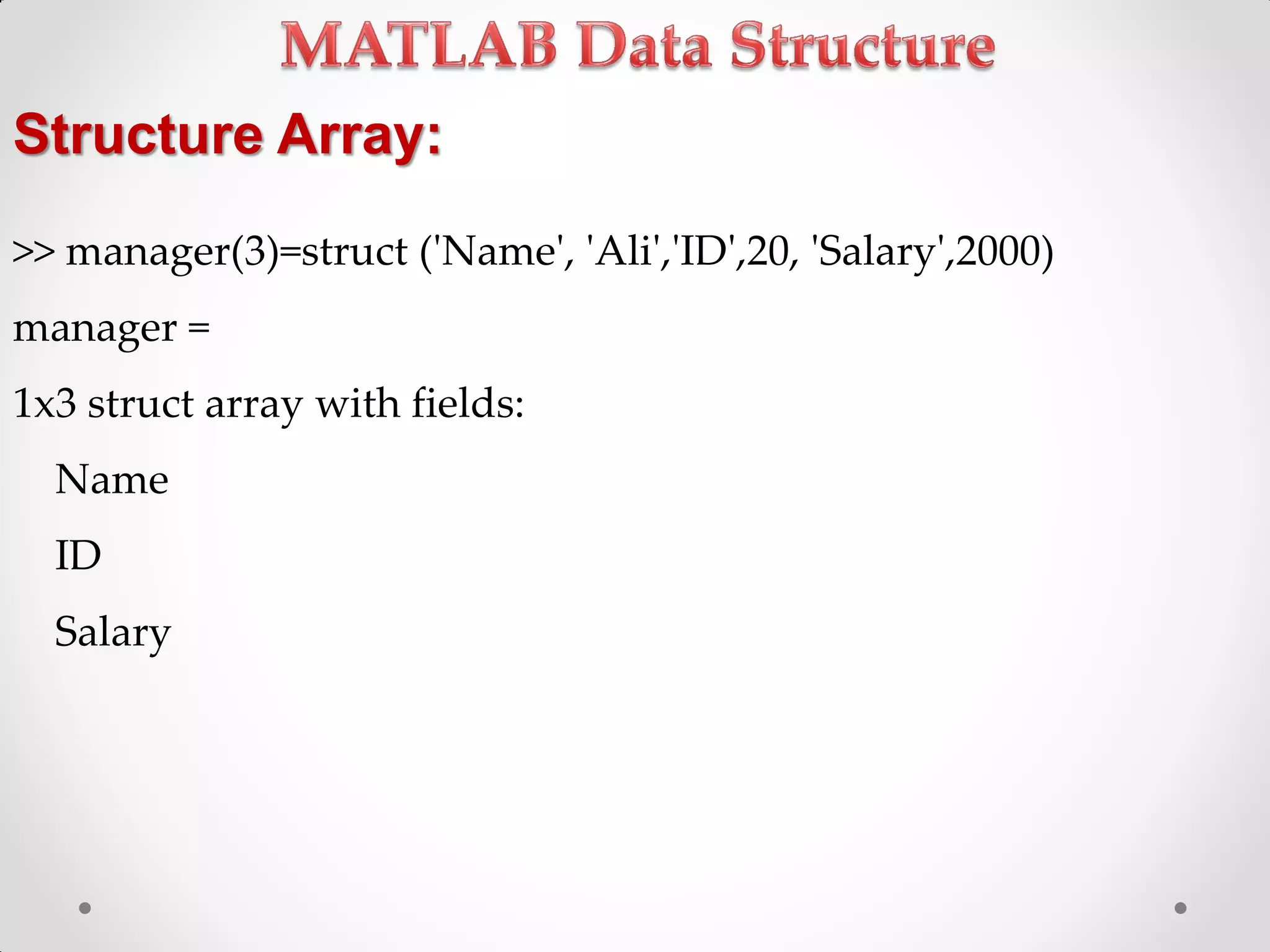
![Structure Array:
• The need of Structure Array
x.y.z = 3
x.y.w = [ 1 2 3]
x.p = ‘hello’
• Note: x can be array](https://image.slidesharecdn.com/matlab-150220160218-conversion-gate01/75/MATLAB-Programming-95-2048.jpg)
![Symbolic Matrix:
>> syms a b c
>> A = [a b c; b c a; c a b]
A =[ a, b, c ]
[ b, c, a ]
[ c, a, b ]
>> sum(A(1,:))
ans = a+b+c
>> sum(A(1,:)) == sum(A(:,2)) % This is a logical test.
ans =1](https://image.slidesharecdn.com/matlab-150220160218-conversion-gate01/75/MATLAB-Programming-99-2048.jpg)
![Symbolic Plots:
• ezplot(...)
• Symbolic expression plot in the 2D
>> y = sin(x)*exp(-0.3*x)
>> ezplot(y,0,10)
• ezmesh(..)
• Symbolic expression plot in the 3D
>> z = sin(a)*exp(-0.3*a)/(cos(b)+2)
>> ezmesh(z,[0 10 0 10])](https://image.slidesharecdn.com/matlab-150220160218-conversion-gate01/75/MATLAB-Programming-101-2048.jpg)
![Differentiation diff :
• Numerical Difference or Symbolic Differentiation
>> z = [1, 3, 5, 7, 9, 11];
>> dz = diff(z)
>> Syms x t
>> x=t^4;
>> xd3 = diff(x,3)](https://image.slidesharecdn.com/matlab-150220160218-conversion-gate01/75/MATLAB-Programming-103-2048.jpg)
![solve equation solve(...):
>> syms x y real
>> eq1 = x+y-5
>> eq2 = x*y-6
>> [xa, ya] = solve(eq1, eq2)
OR
>> answer = solve(eq1, eq2)
answer.x
answer.y
>> syms x y real
>> s = solve('x+y=9','x*y=20')](https://image.slidesharecdn.com/matlab-150220160218-conversion-gate01/75/MATLAB-Programming-106-2048.jpg)
![Differential Equations dsolve(..):
• Symbolic solution of ordinary differential equations
>> syms x real
>> diff_eq_sol = dsolve('m*D2x+b*Dx+k*x=0','Dx(0)=-1','x(0)=2')
>> syms m b k real
>> subs(diff_eq_sol, [m,b,k], [2,5,100])](https://image.slidesharecdn.com/matlab-150220160218-conversion-gate01/75/MATLAB-Programming-107-2048.jpg)


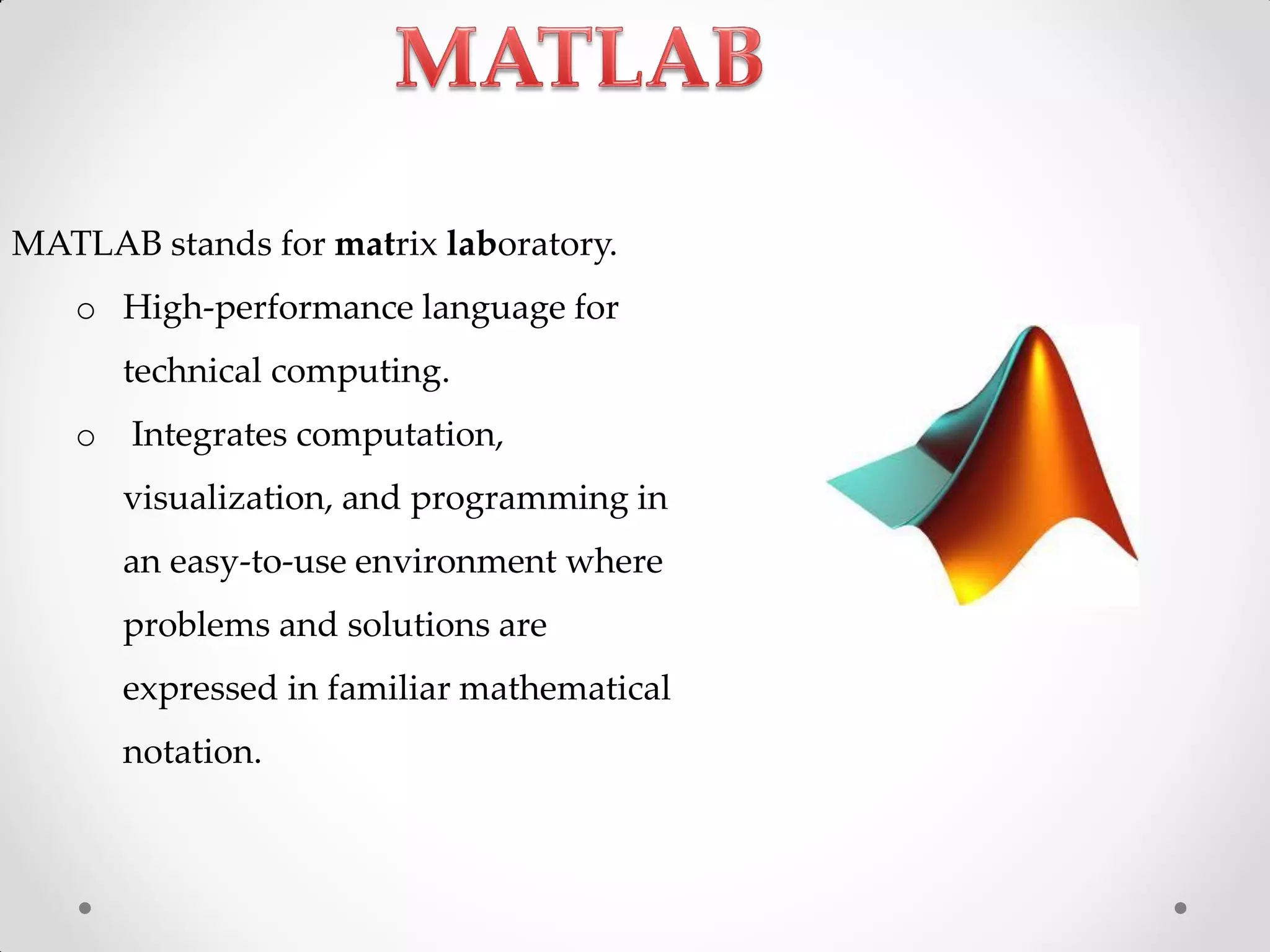
This document provides an overview of MATLAB including its history, applications, development environment, built-in functions, and toolboxes. MATLAB stands for Matrix Laboratory and was originally developed in the 1970s at the University of New Mexico to provide an interactive environment for matrix computations. It has since grown to be a comprehensive programming language and environment used widely in technical computing across many domains including engineering, science, and finance. The key components of MATLAB are its development environment, mathematical function library, programming language, graphics capabilities, and application programming interface. It also includes a variety of toolboxes that provide domain-specific functionality in areas like signal processing, neural networks, and optimization.
Introduction of Mohamed Abd Elhay, a professional Embedded Software Engineer.
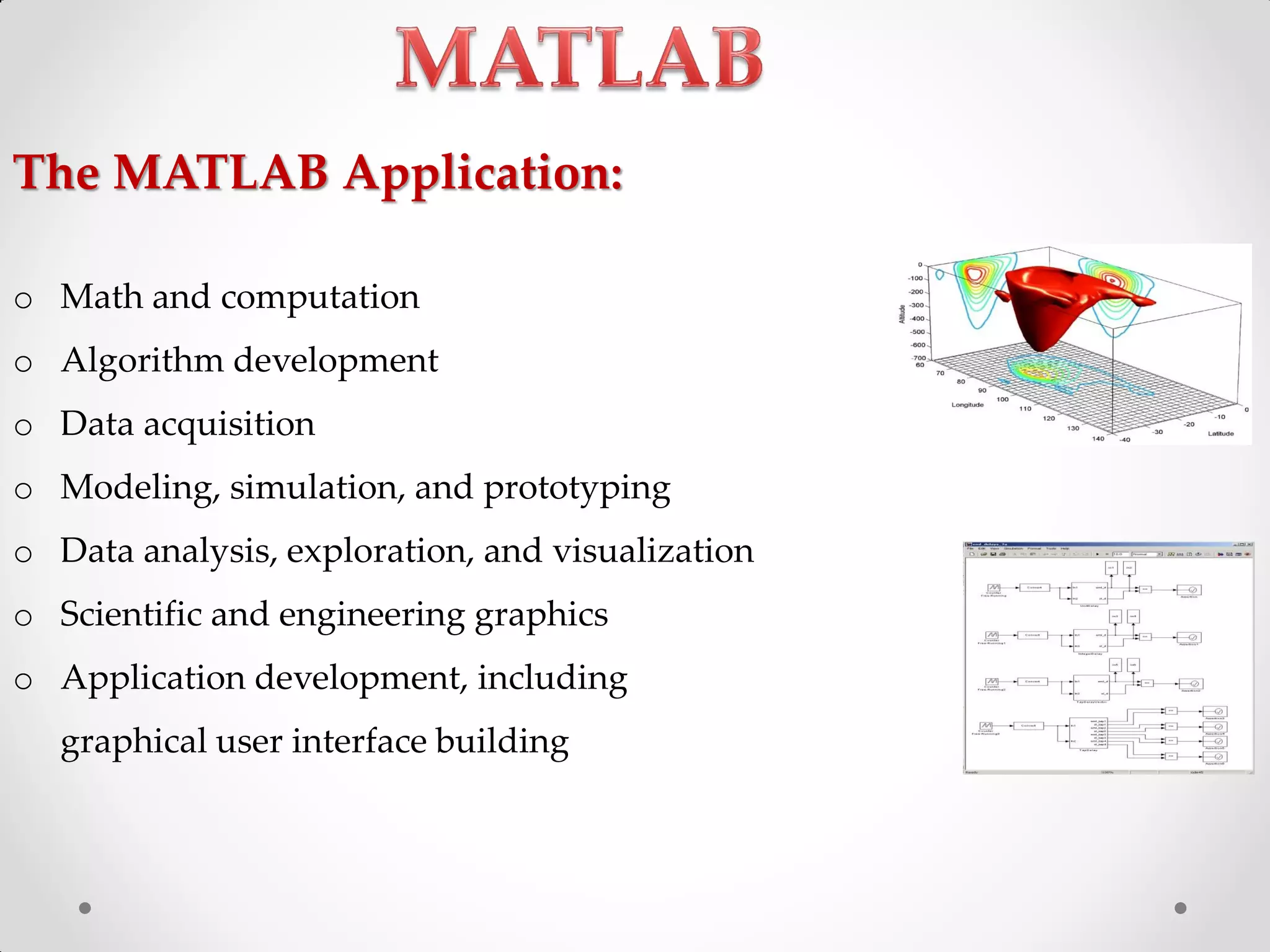
An introduction to MATLAB, its applications, including technical computing, visualization, and programming.
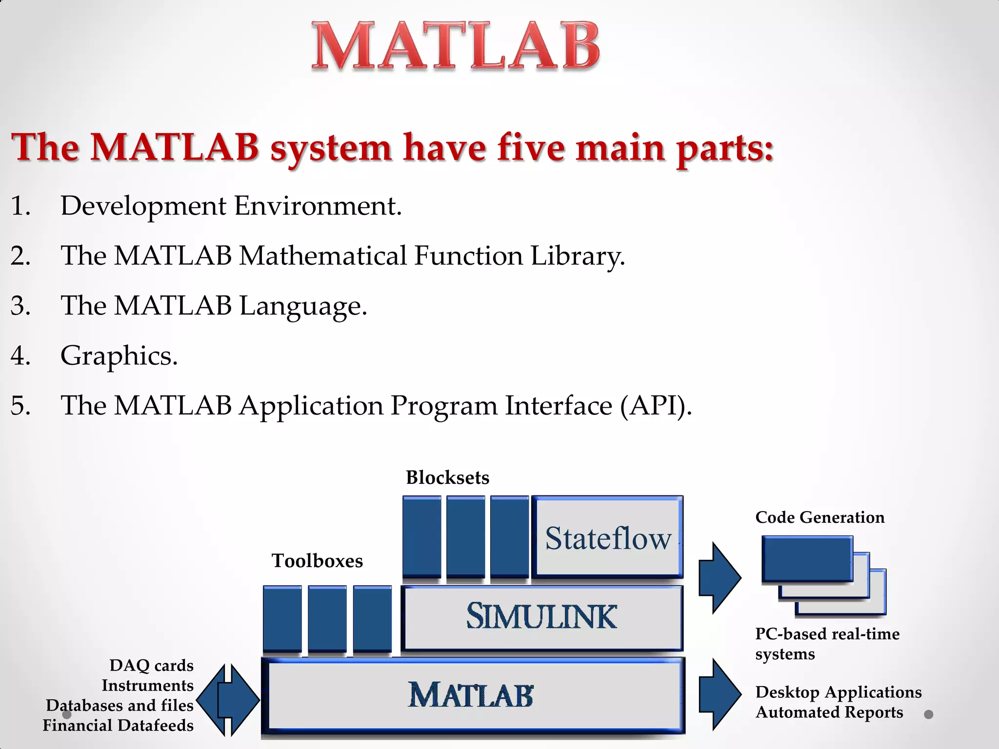
Overview of the main components of MATLAB: Development Environment, Function Library, Language, Graphics, and API.
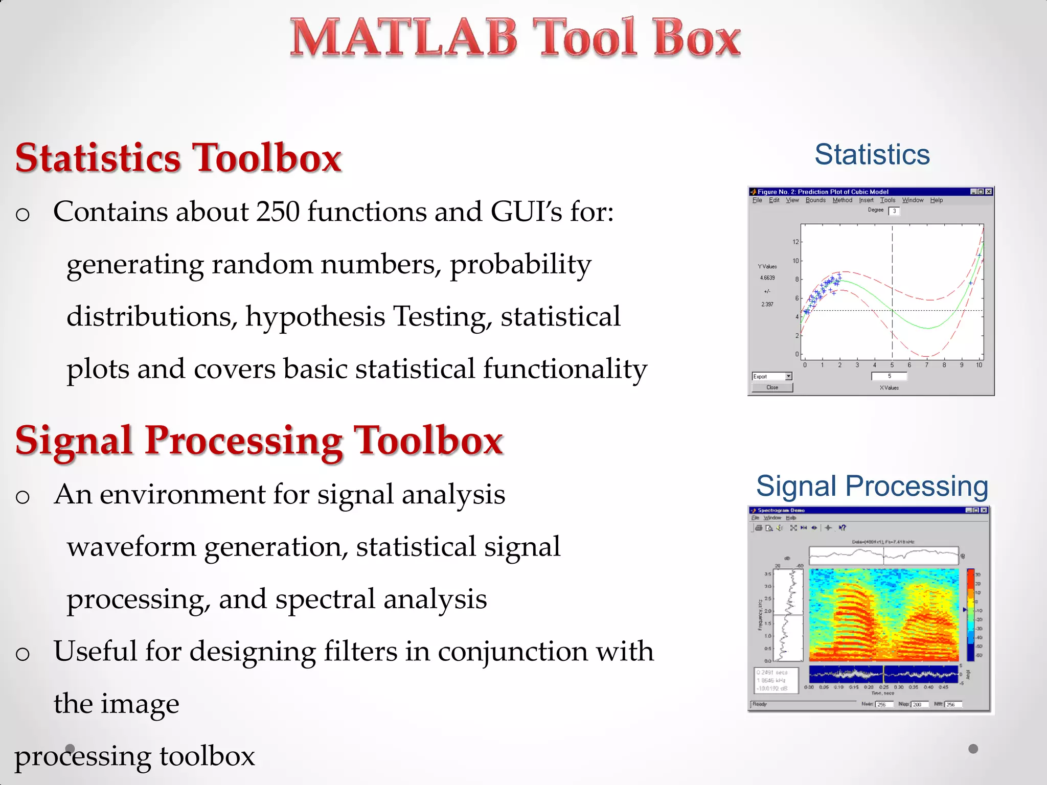
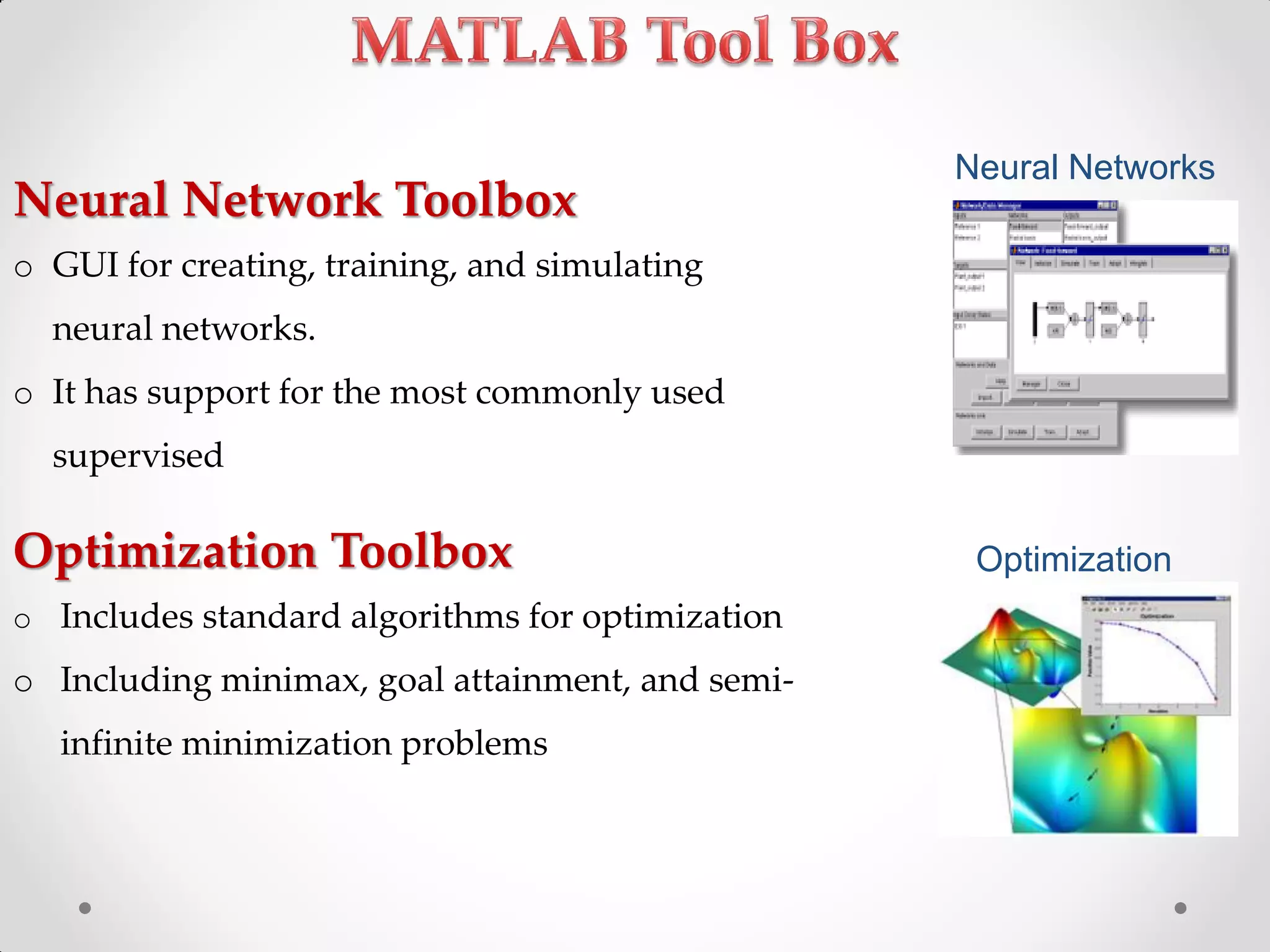
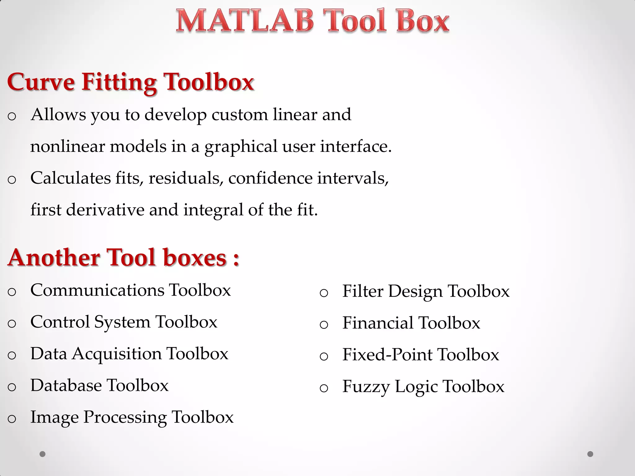
Various MATLAB toolboxes such as Statistics, Signal Processing, Neural Network, Optimization, and Curve Fitting.
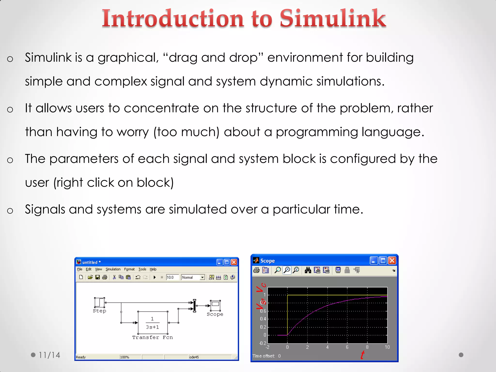
Introduction to Simulink for dynamic simulations, emphasizing its graphical environment which simplifies modeling.
.fig, .m, .mat, .mex - different file types used in MATLAB for functions, data storage, and executables.
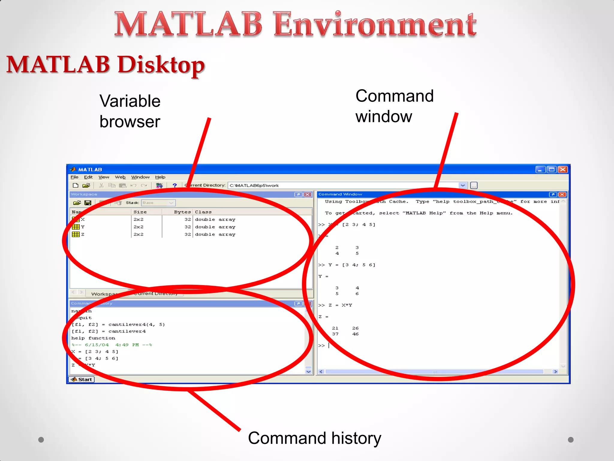
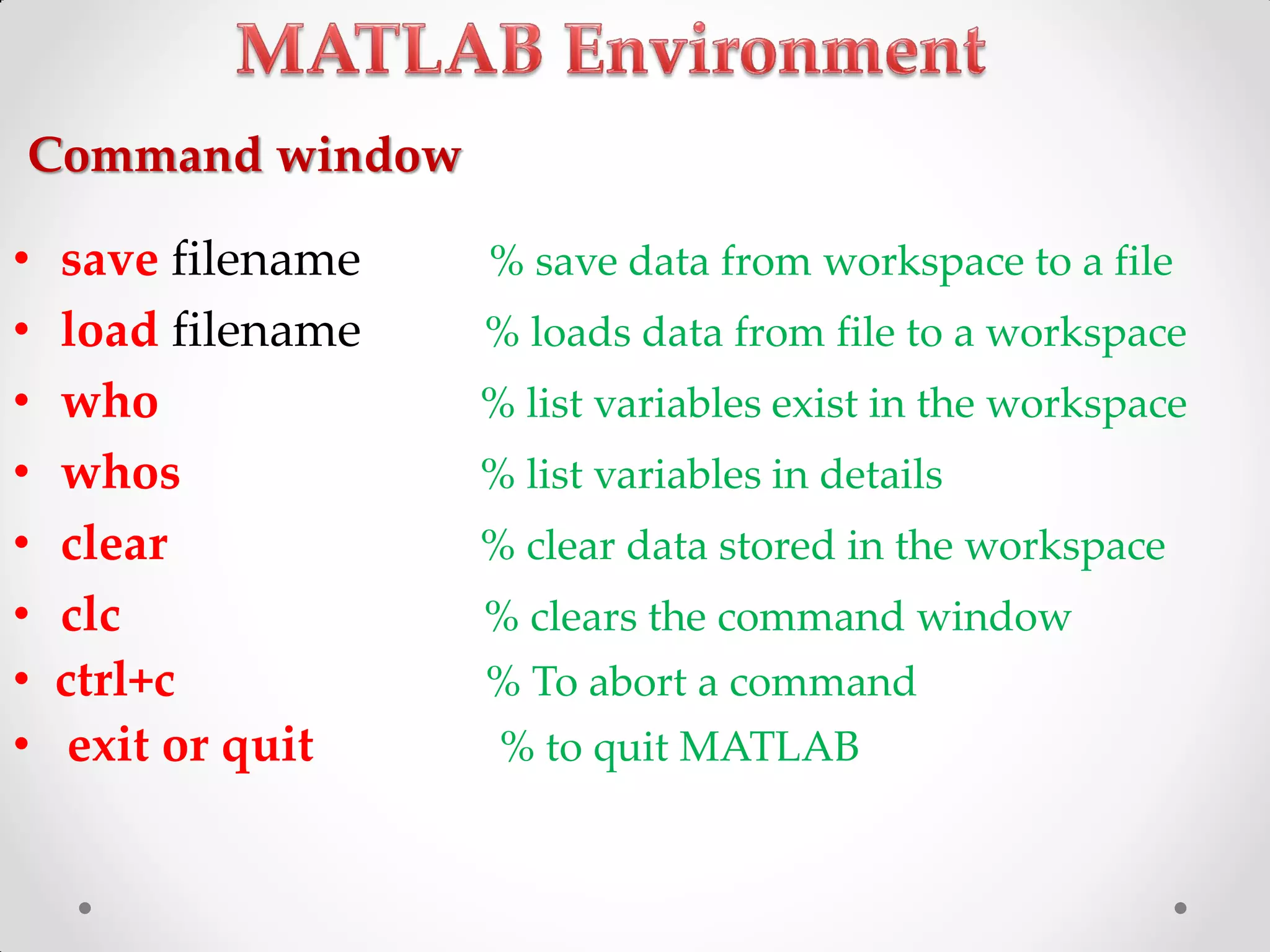
Basic commands for data management in the command window, including listing, loading, saving data.
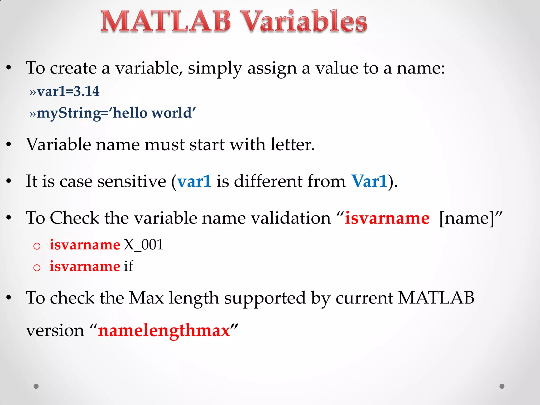
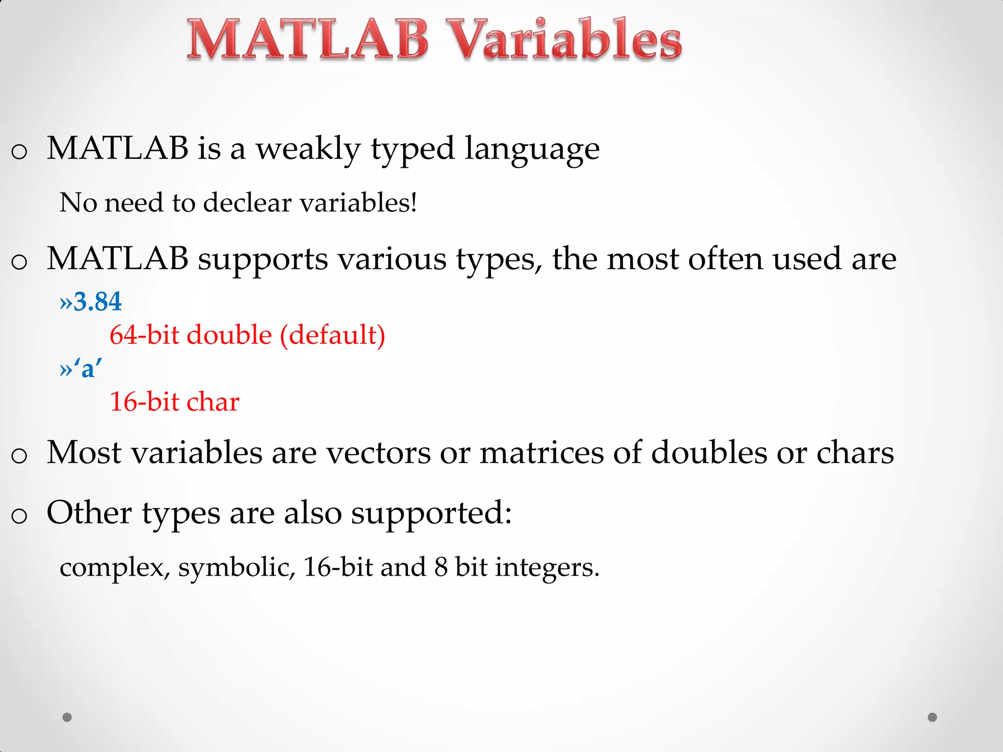
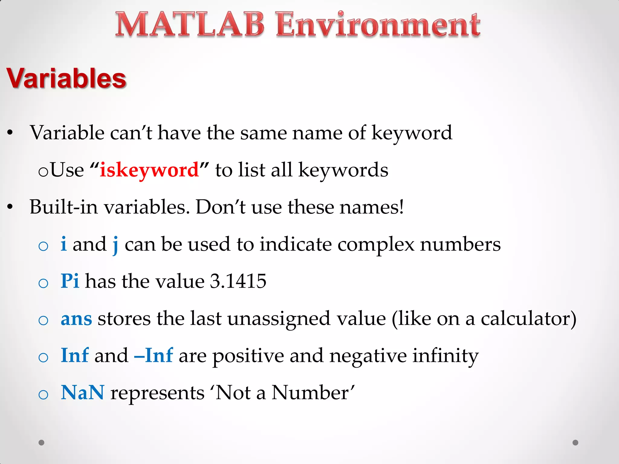
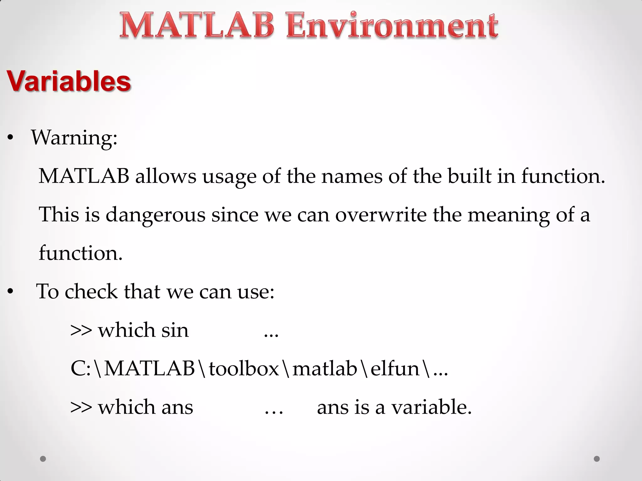
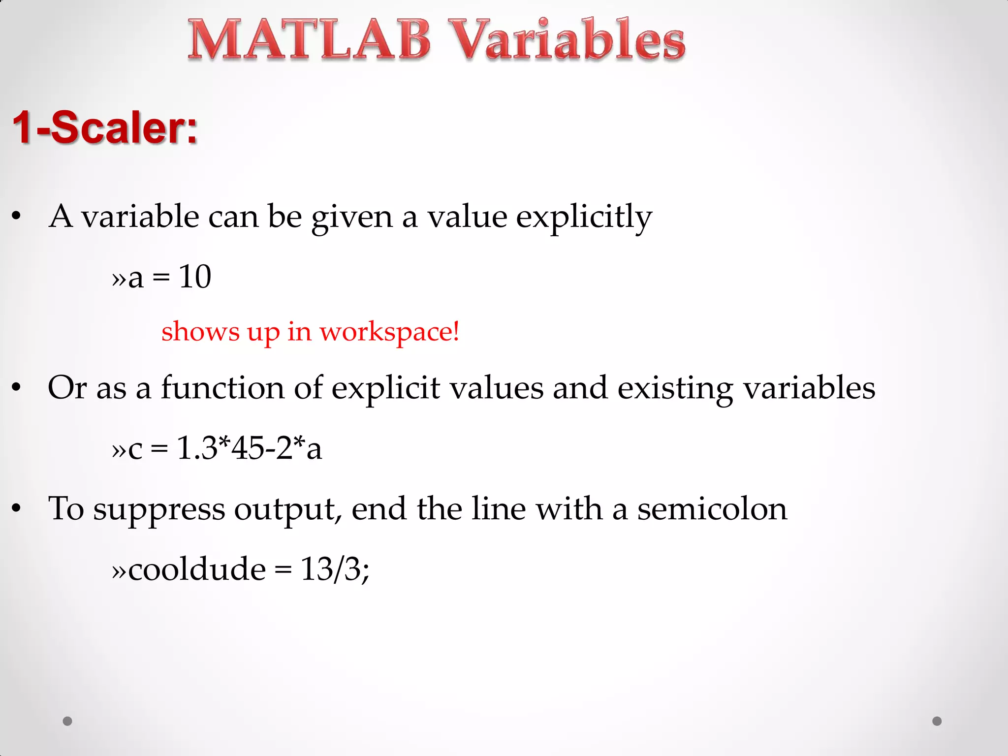
Definition, management, and types of variables in MATLAB, including naming conventions and built-in variables.
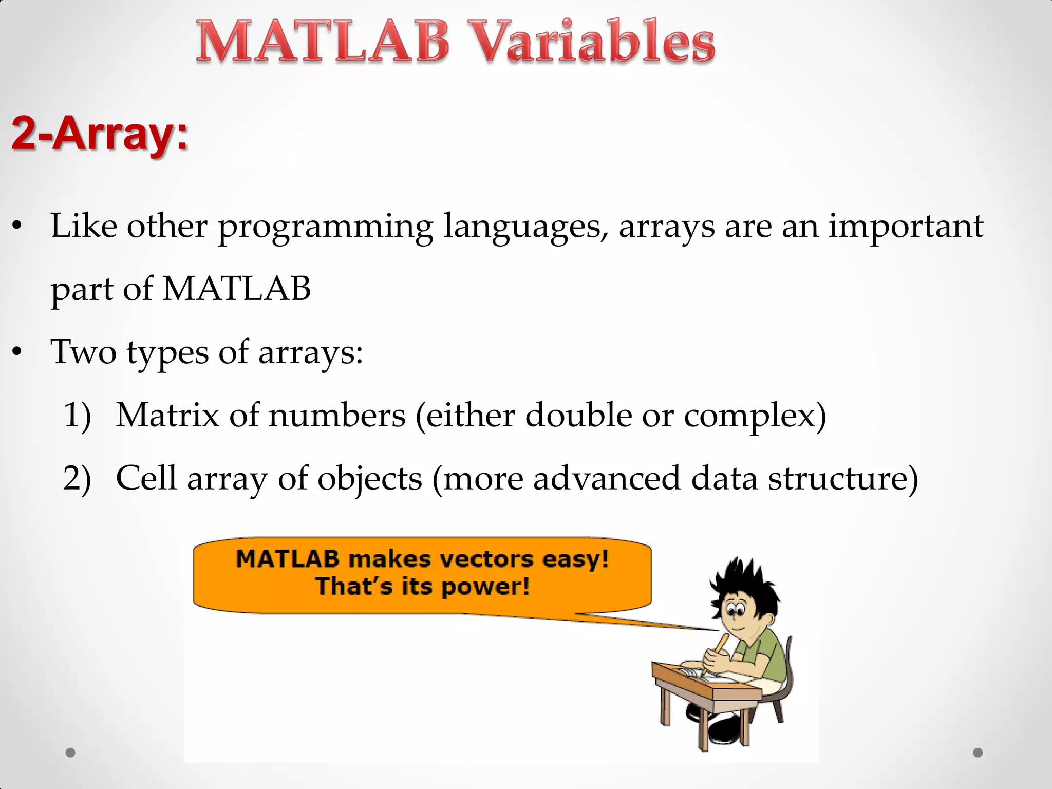
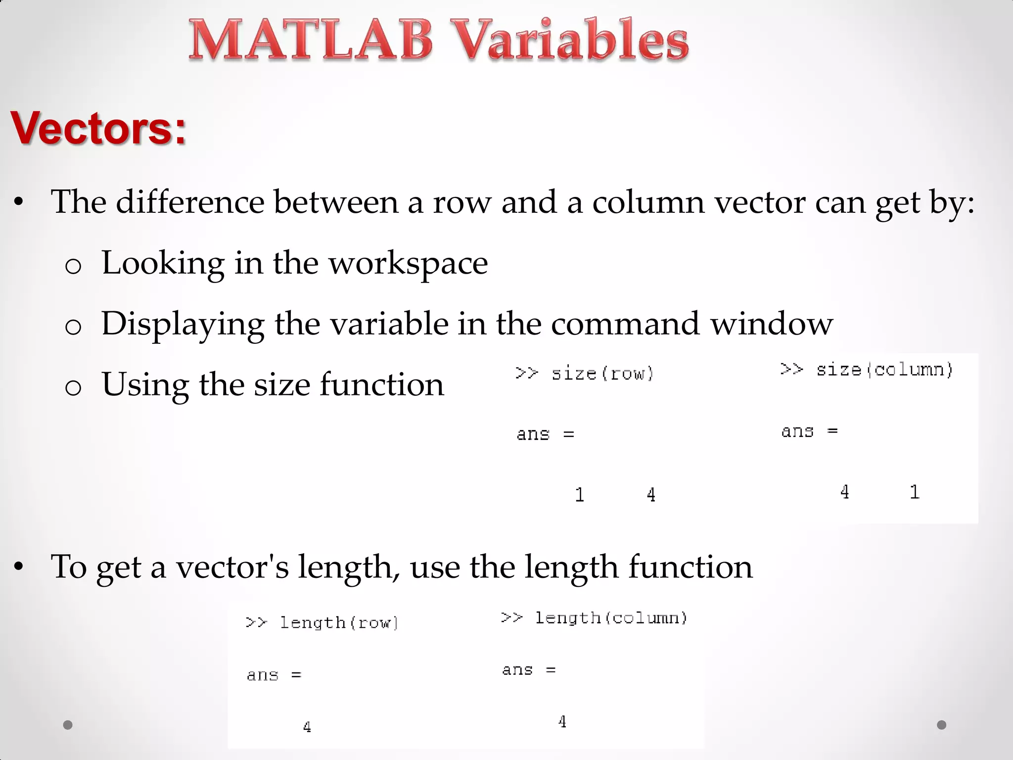
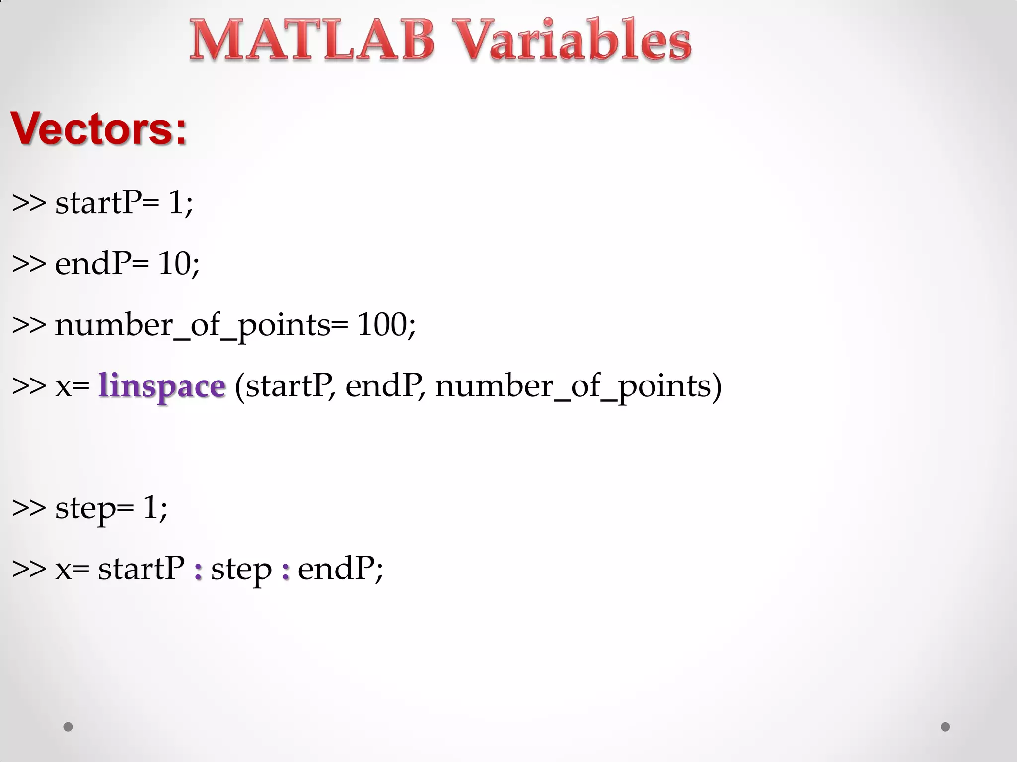
Creating and manipulating arrays, vectors, and matrices in MATLAB including different types.
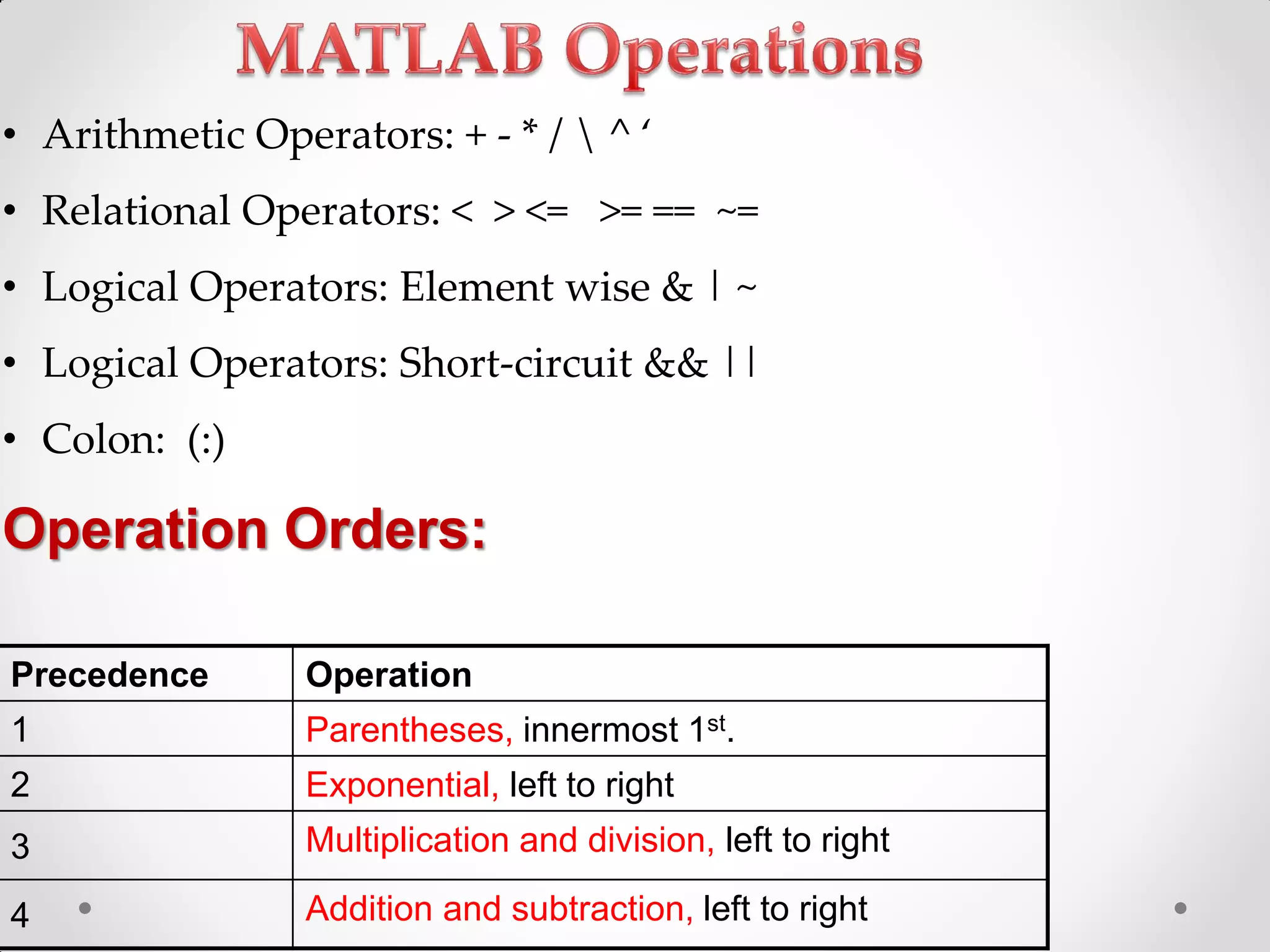
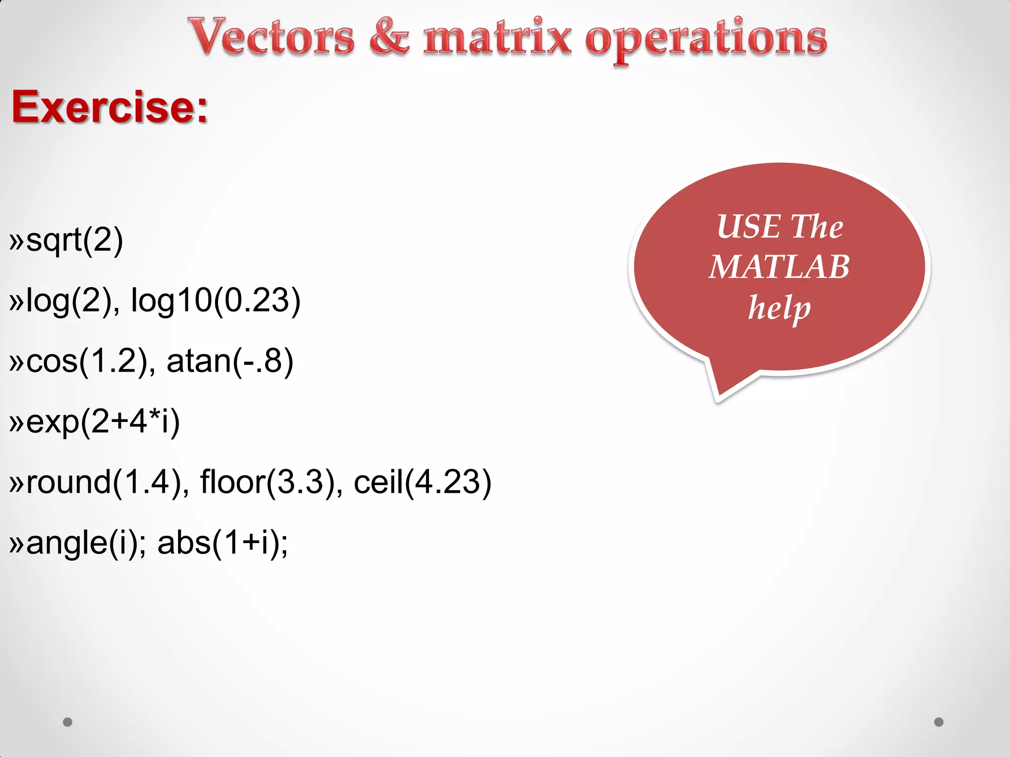
Arithmetic, relational and logical operations in MATLAB along with function examples for data analysis.
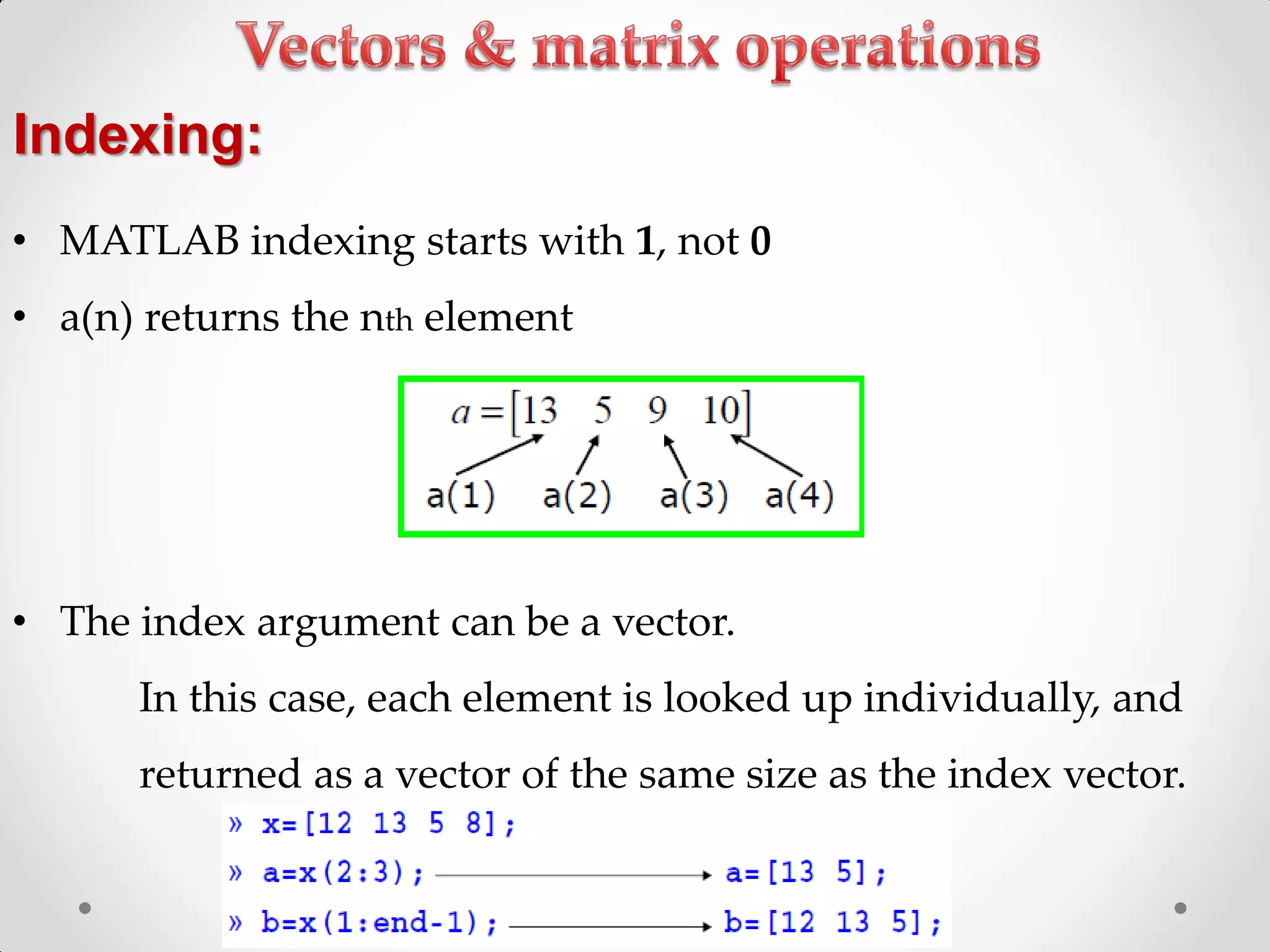
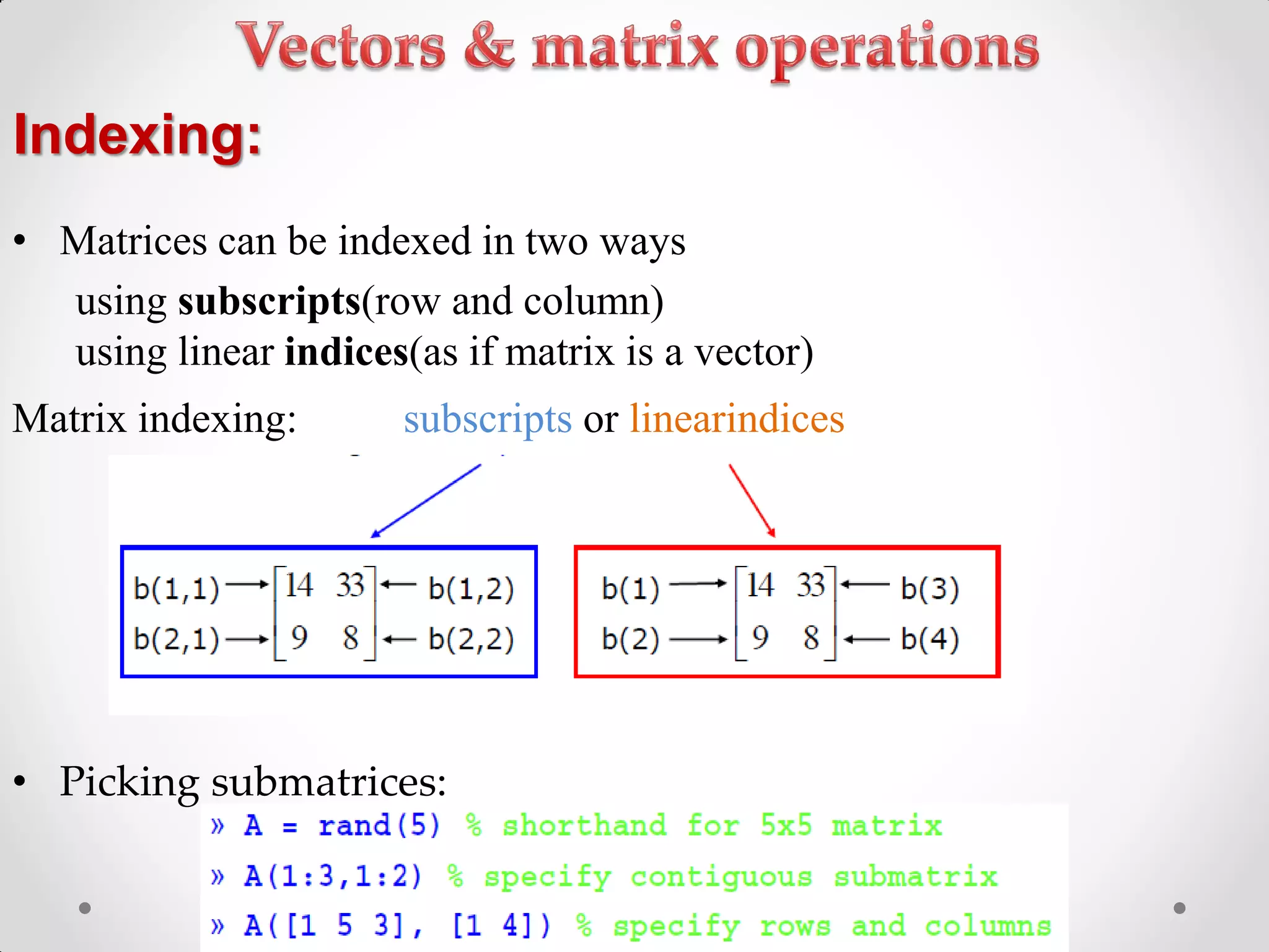
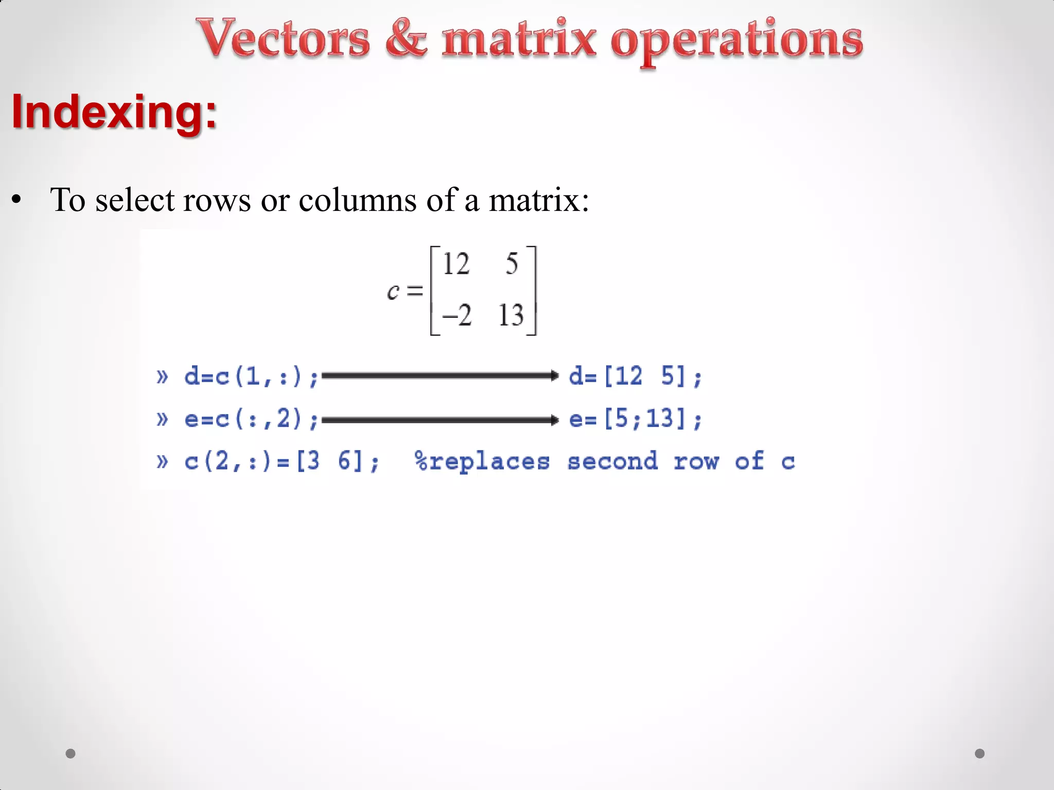
Methods for indexing matrices and data structures, including selection and deletion of matrix elements.
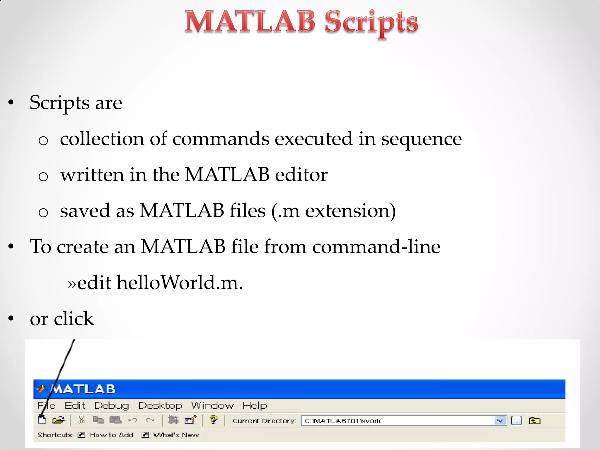
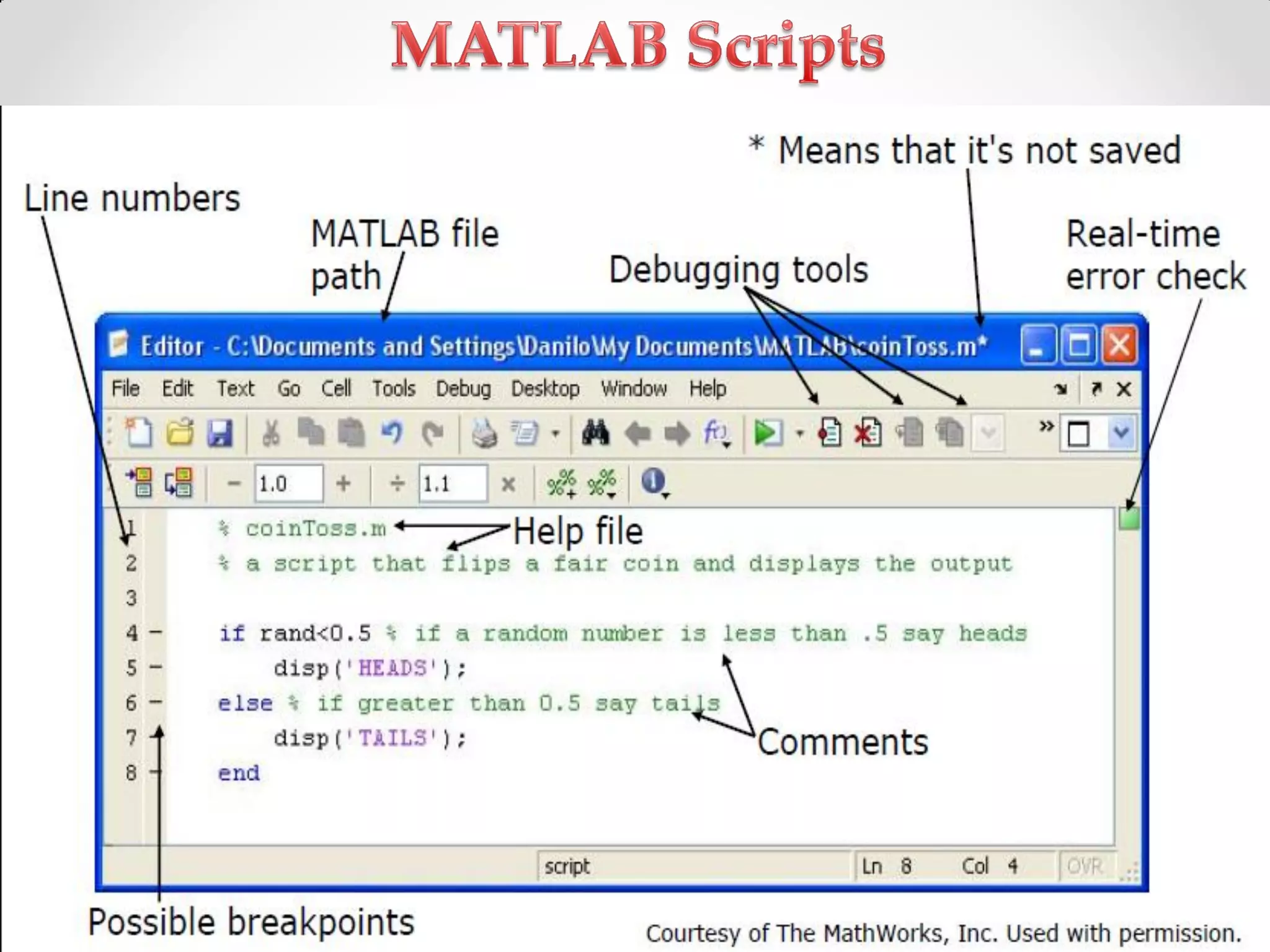
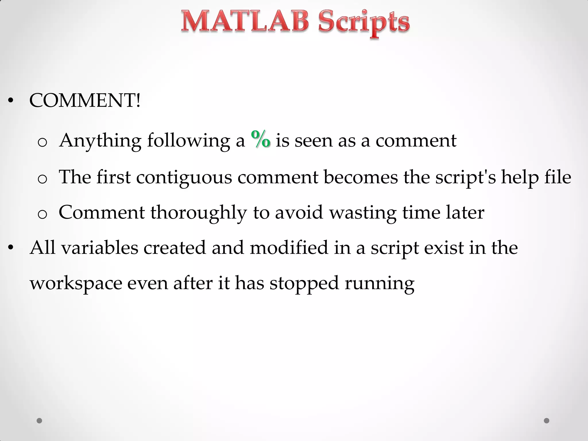
Writing and executing scripts in MATLAB, along with the importance of comments and syntax.
Writing and executing scripts in MATLAB, along with the importance of comments and syntax.
Generating random salary data for employees, statistical analysis (max, min salaries, employee IDs).
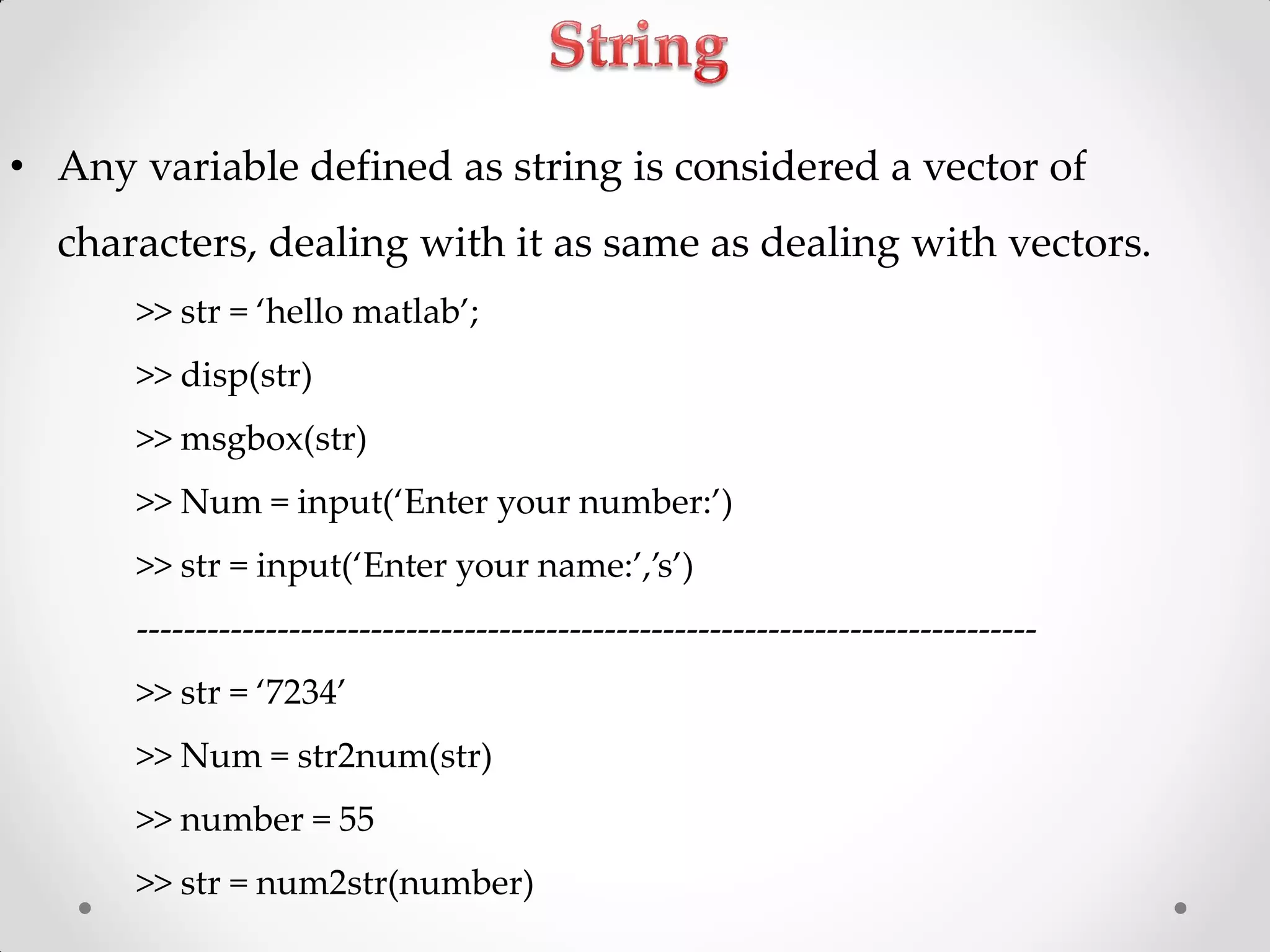
Handling strings in MATLAB and converting between string and numeric formats.
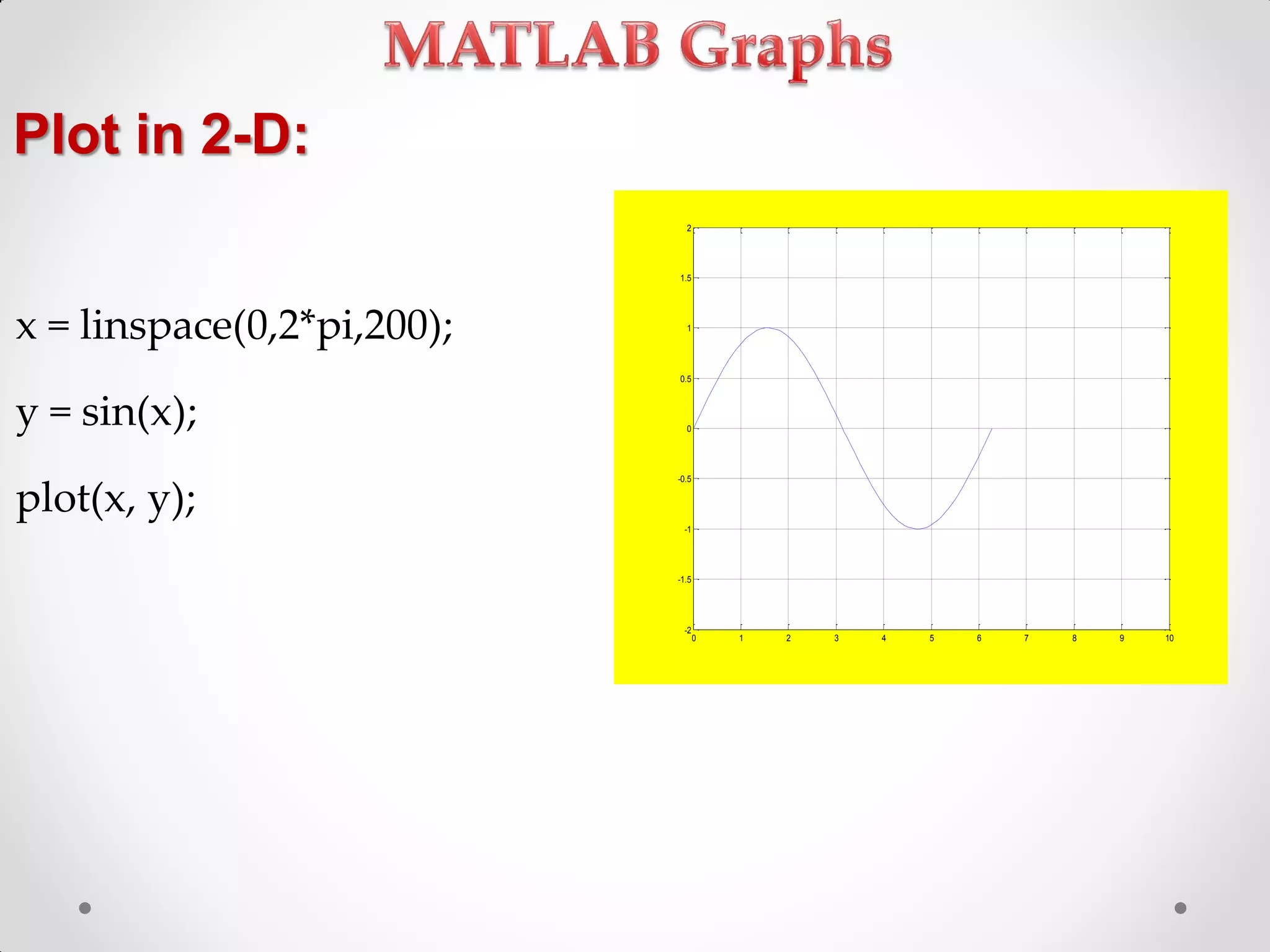
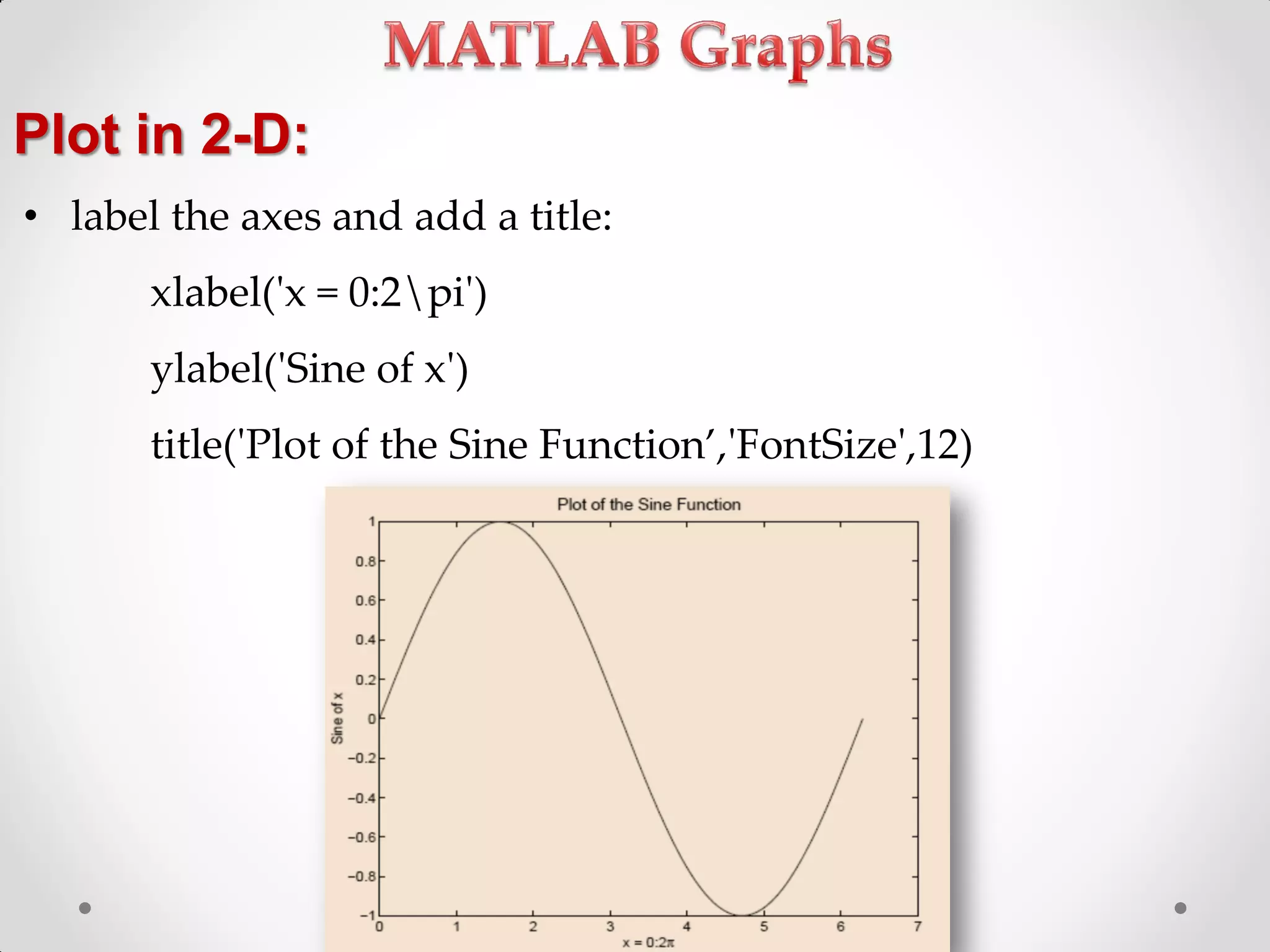
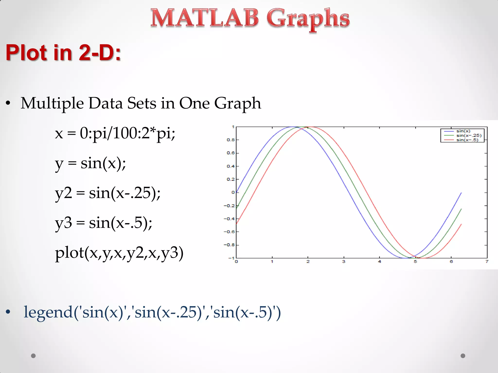
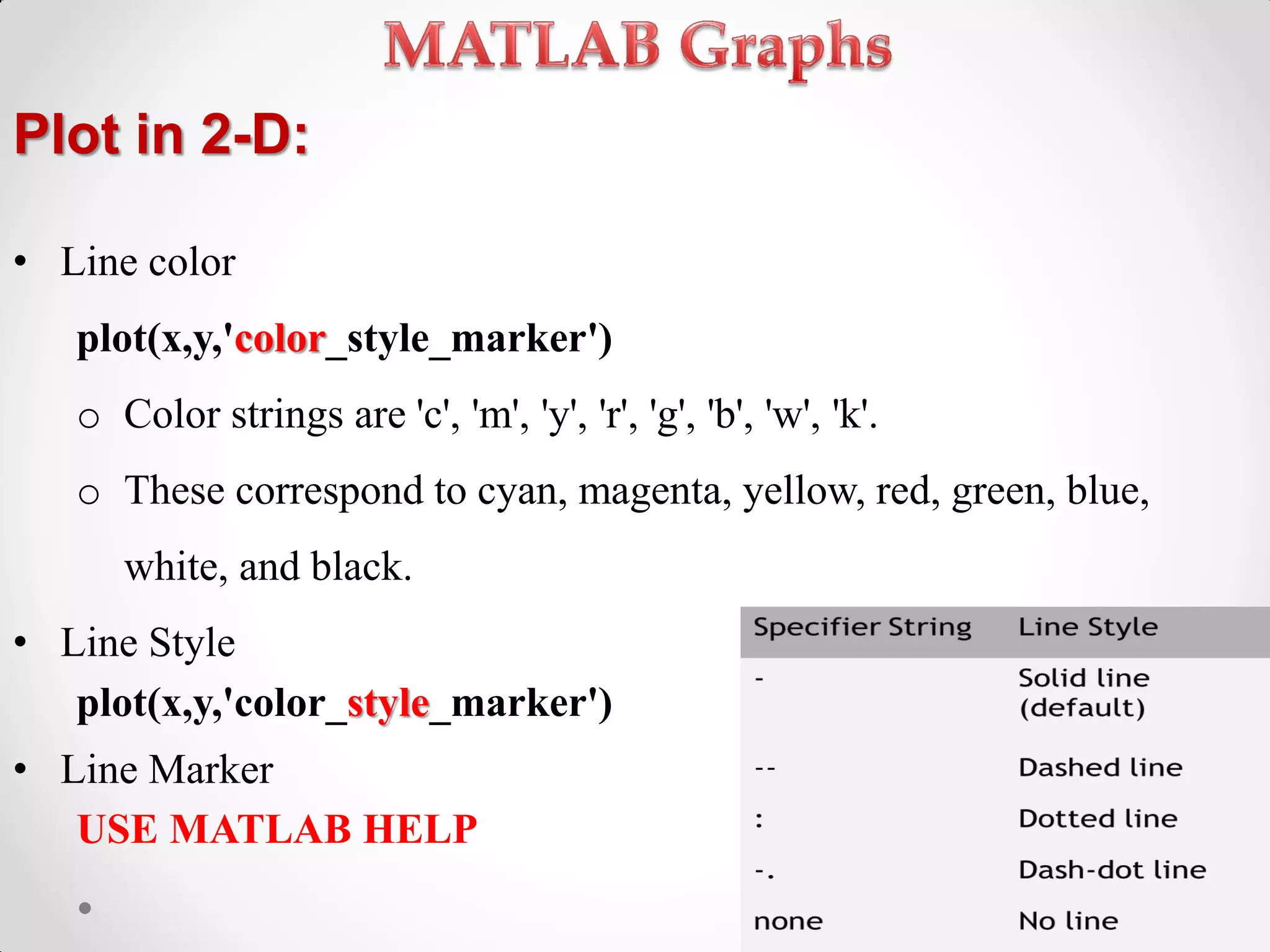
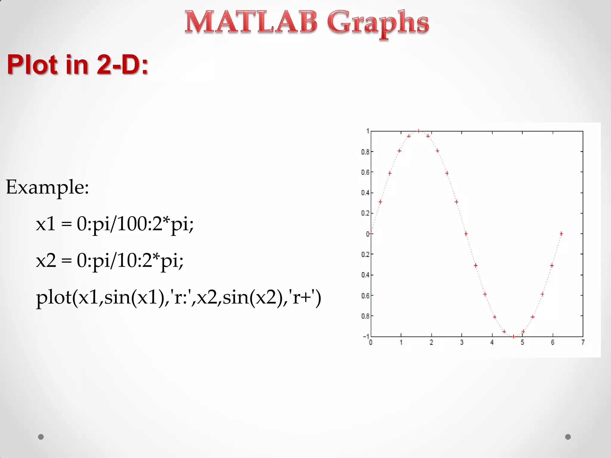
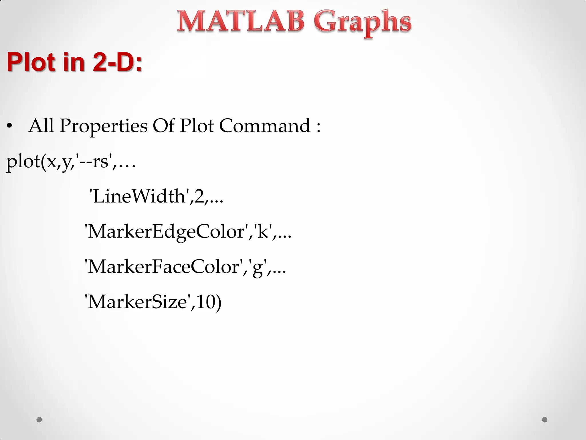
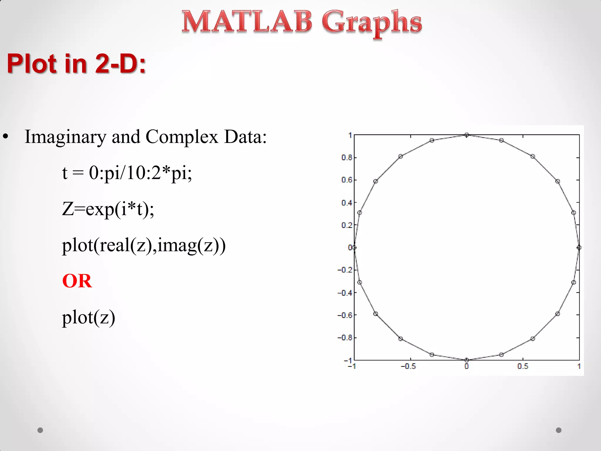
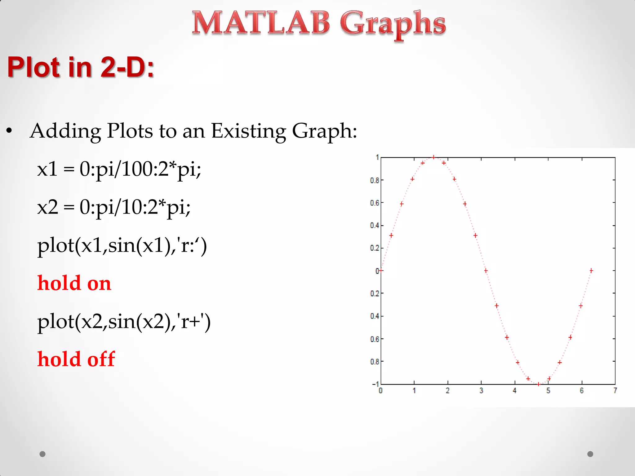
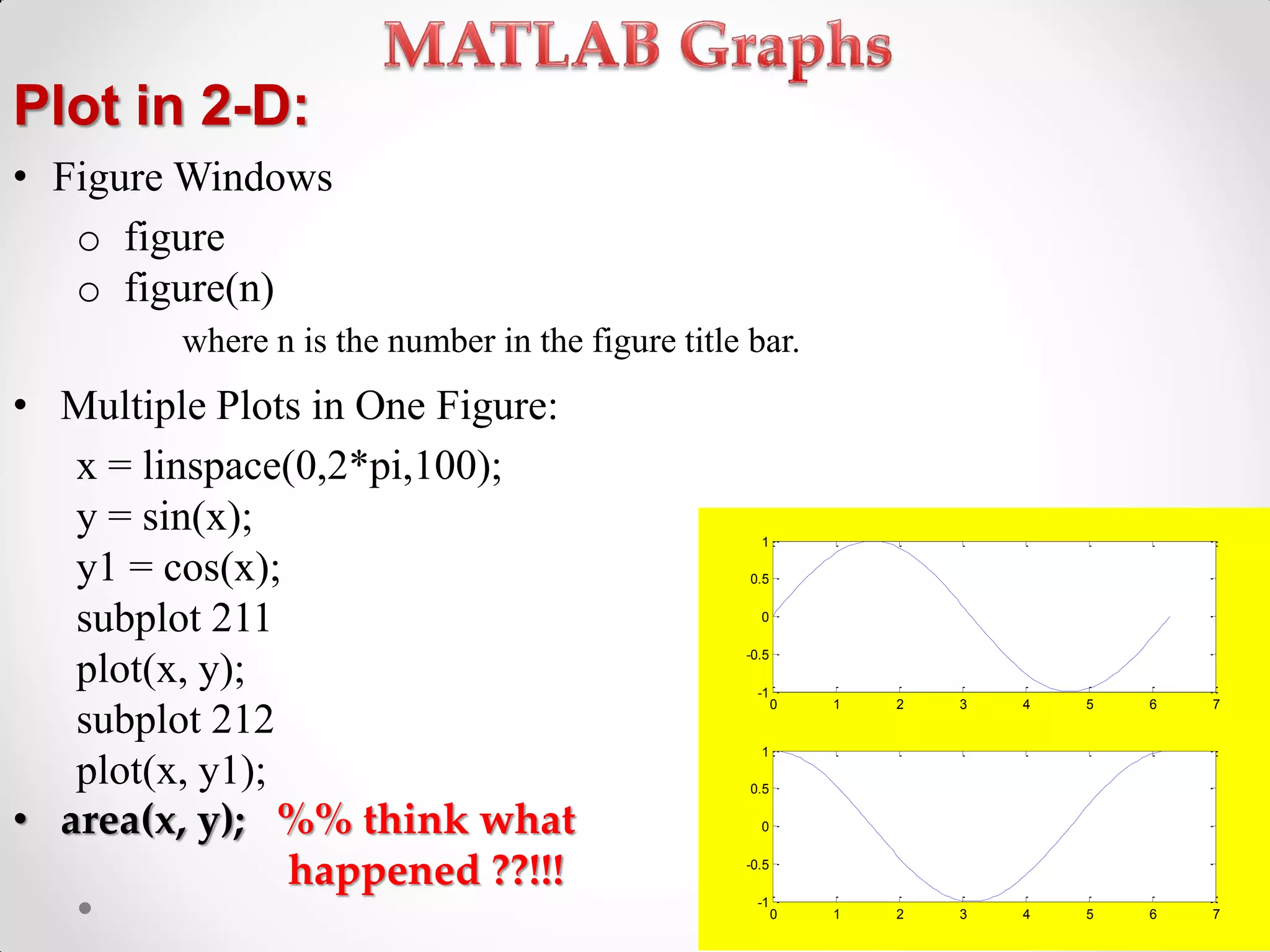
Creating various types of 2D plots (including multiple datasets) and customizing plot appearances.
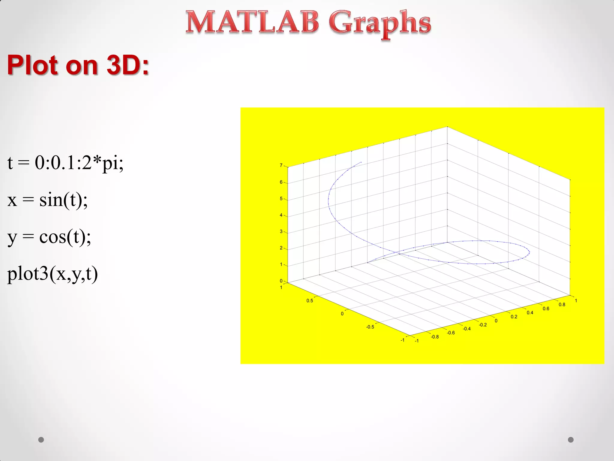
Introduction to 3D plotting in MATLAB with examples for surface and mesh plots.
Using specialized functions for different types of plots and controlling axis properties.
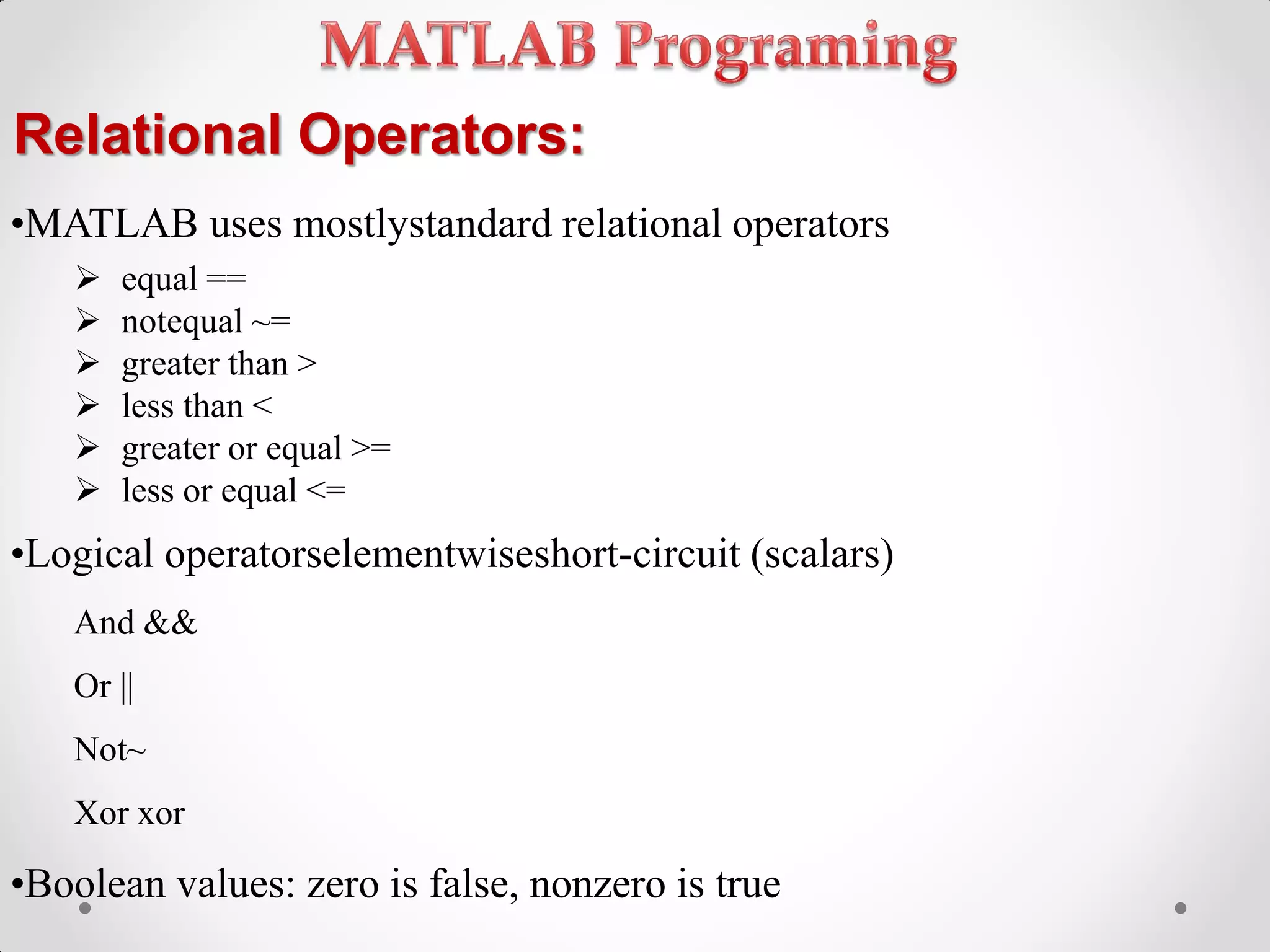
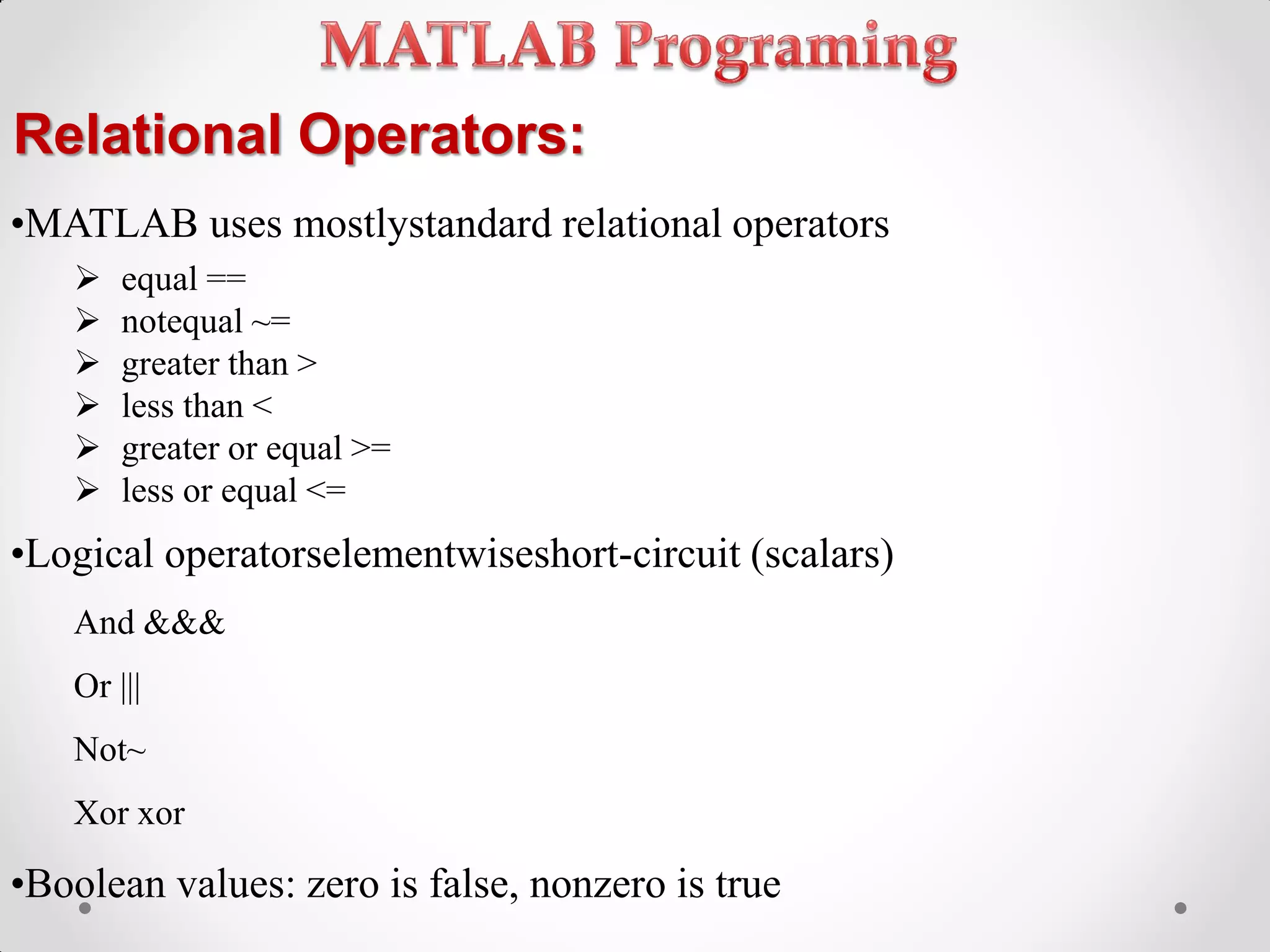
Understanding relational and logical operators in MATLAB along with their functionality.
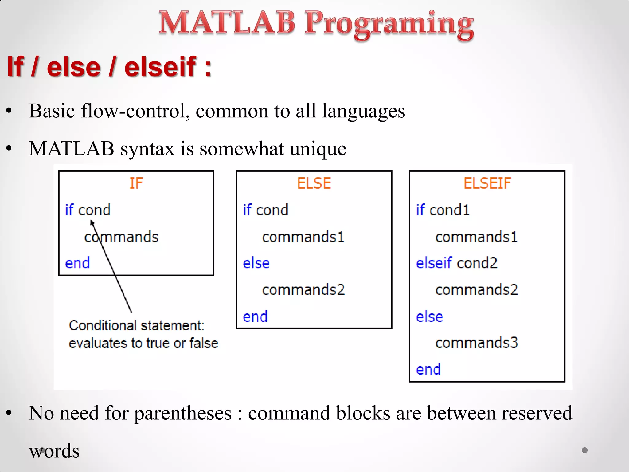
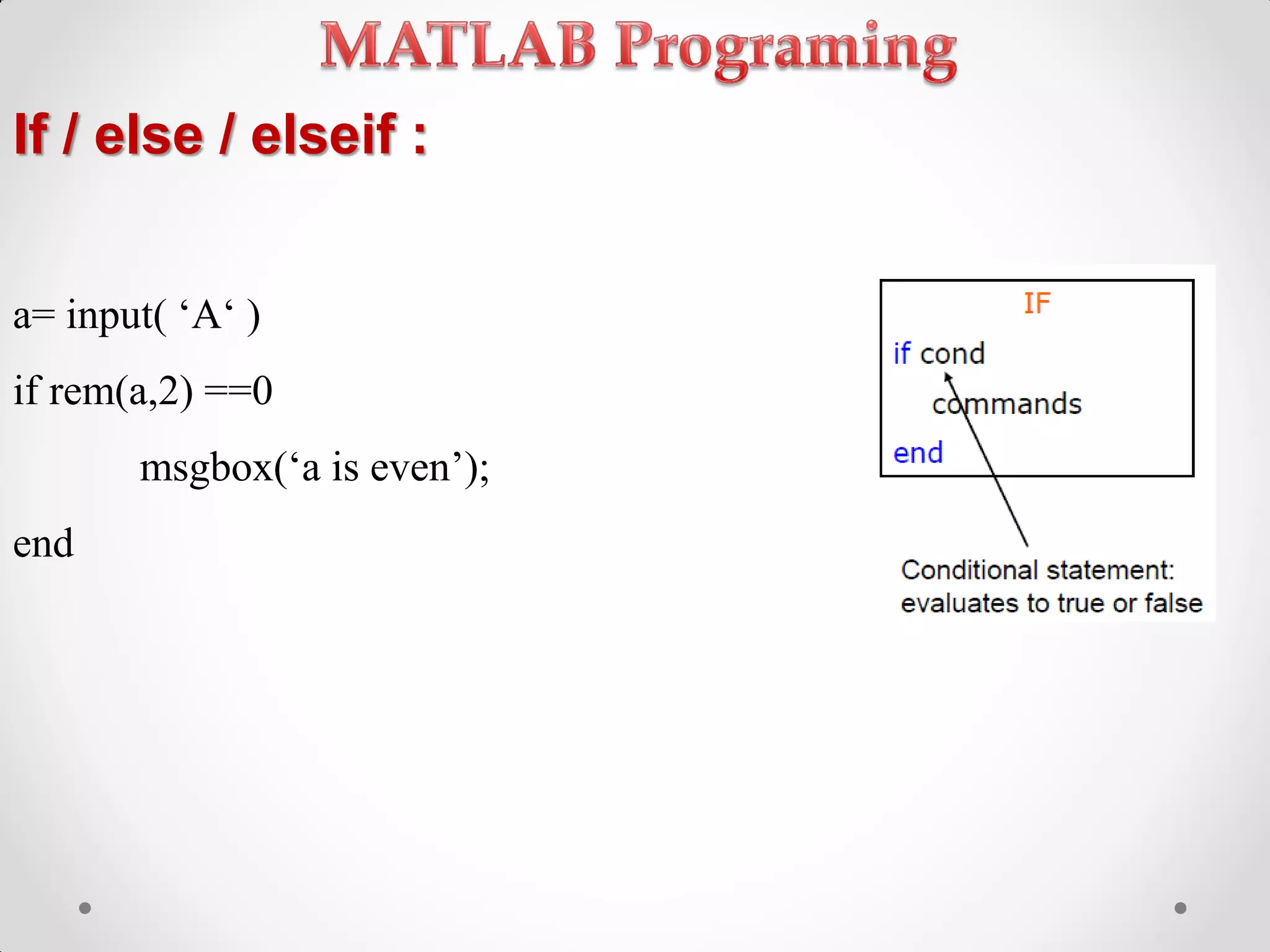
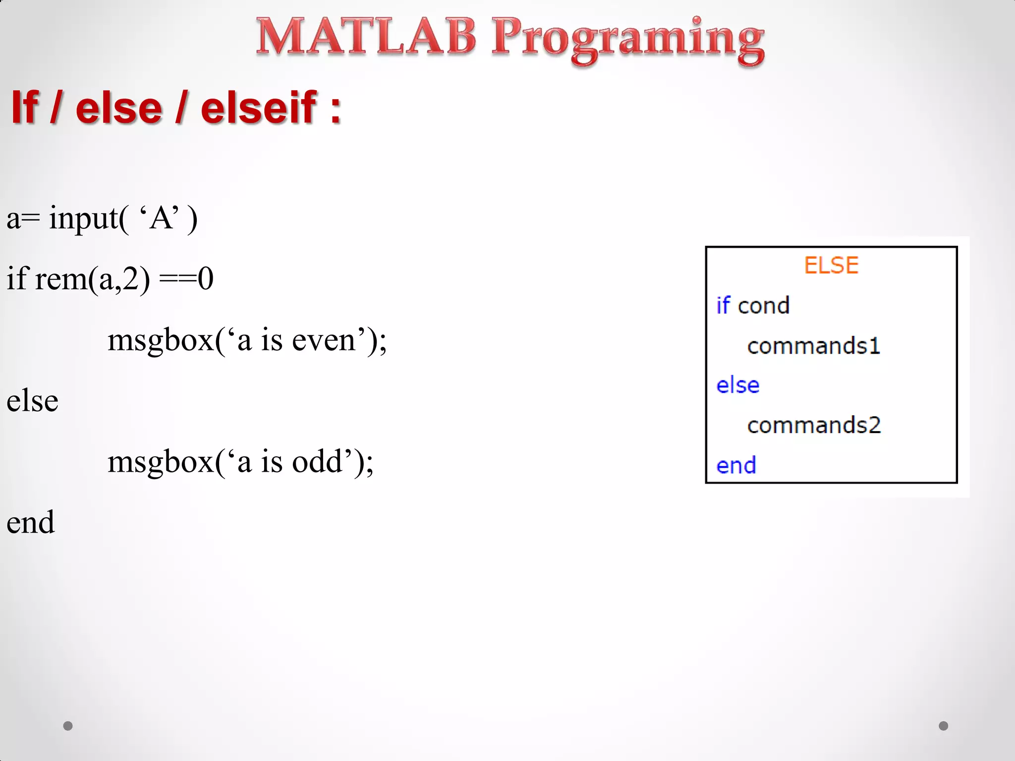
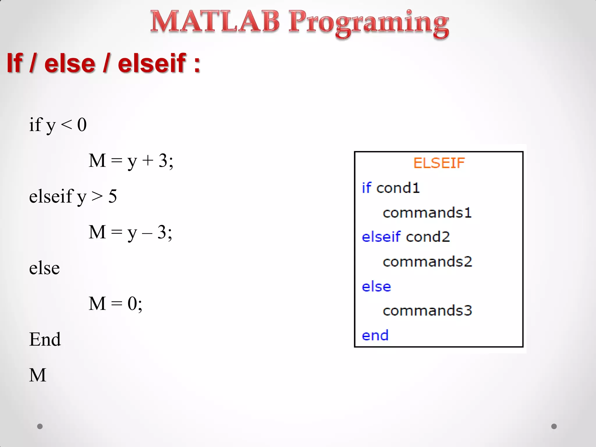
Control flow statements including if, else, and elseif constructs in MATLAB.
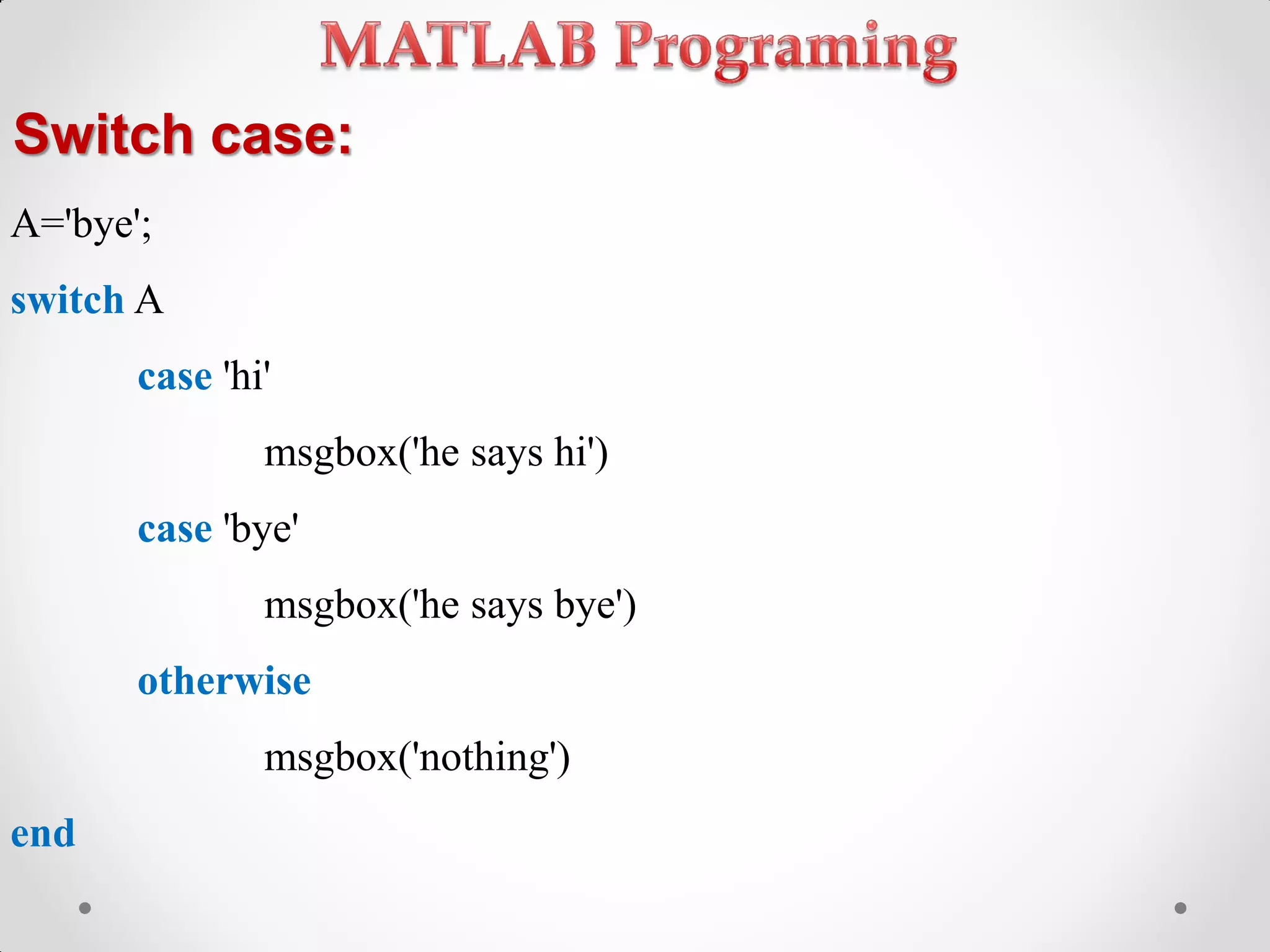
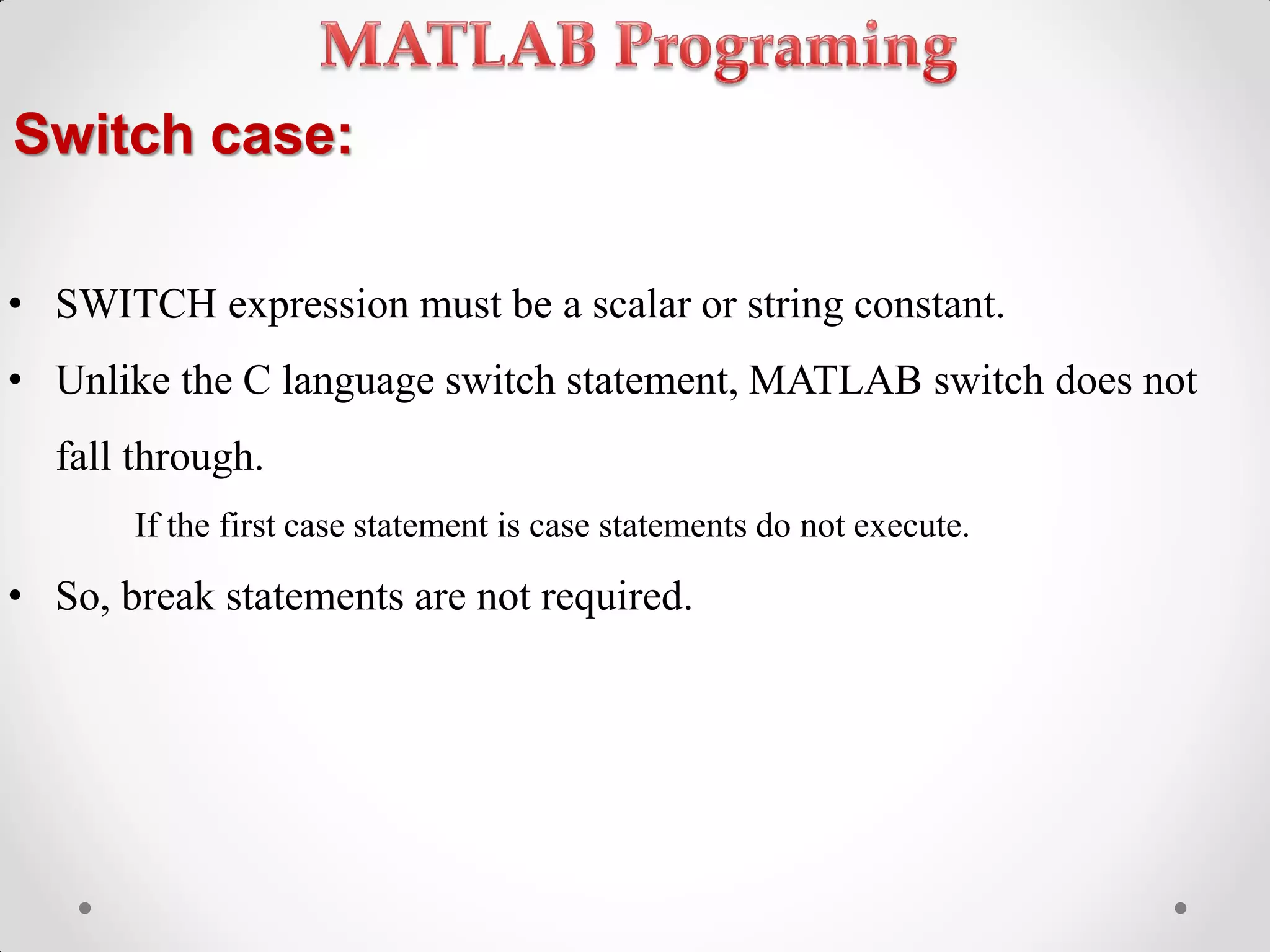
Implementation of switch-case for control flow in MATLAB.
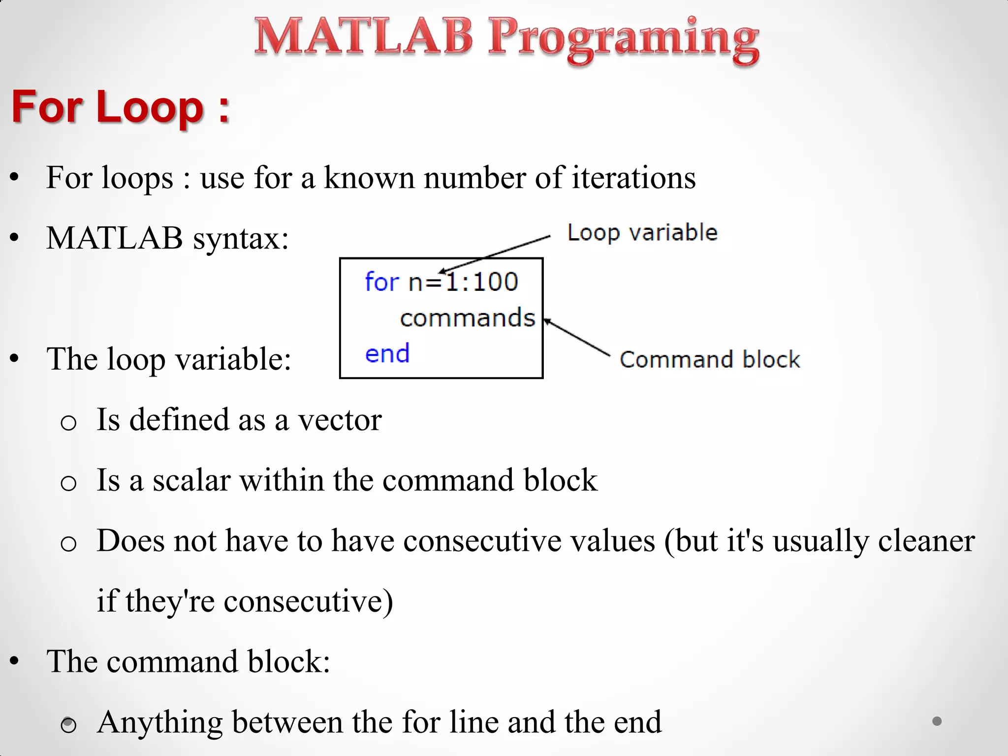
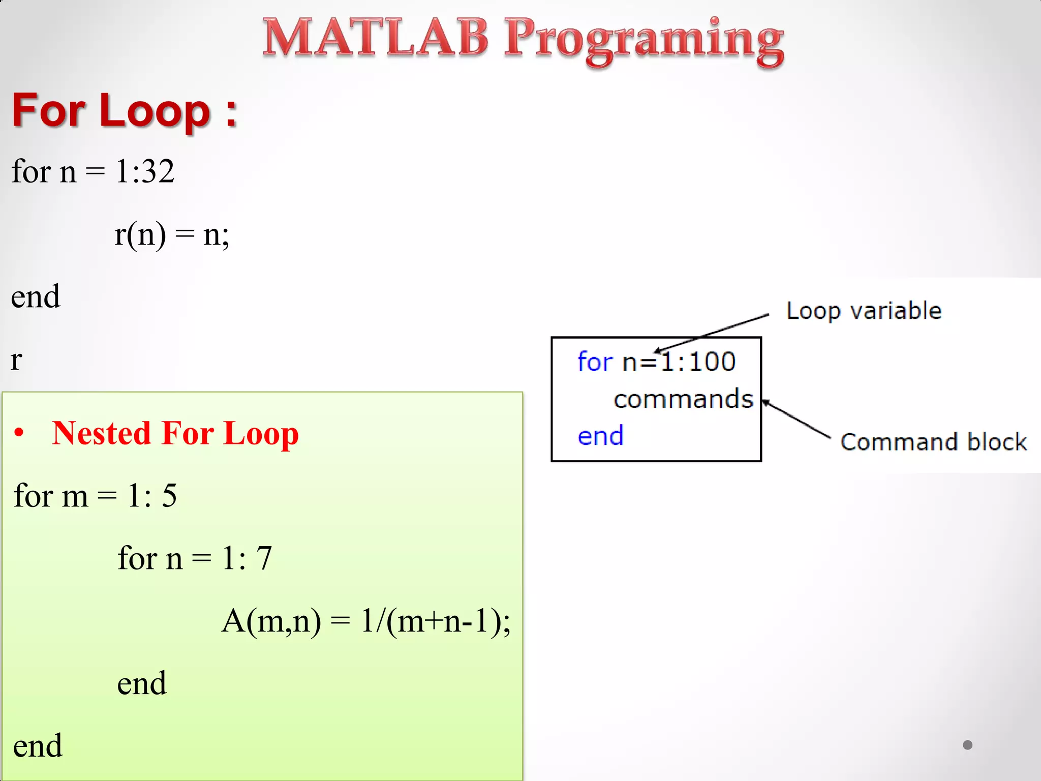
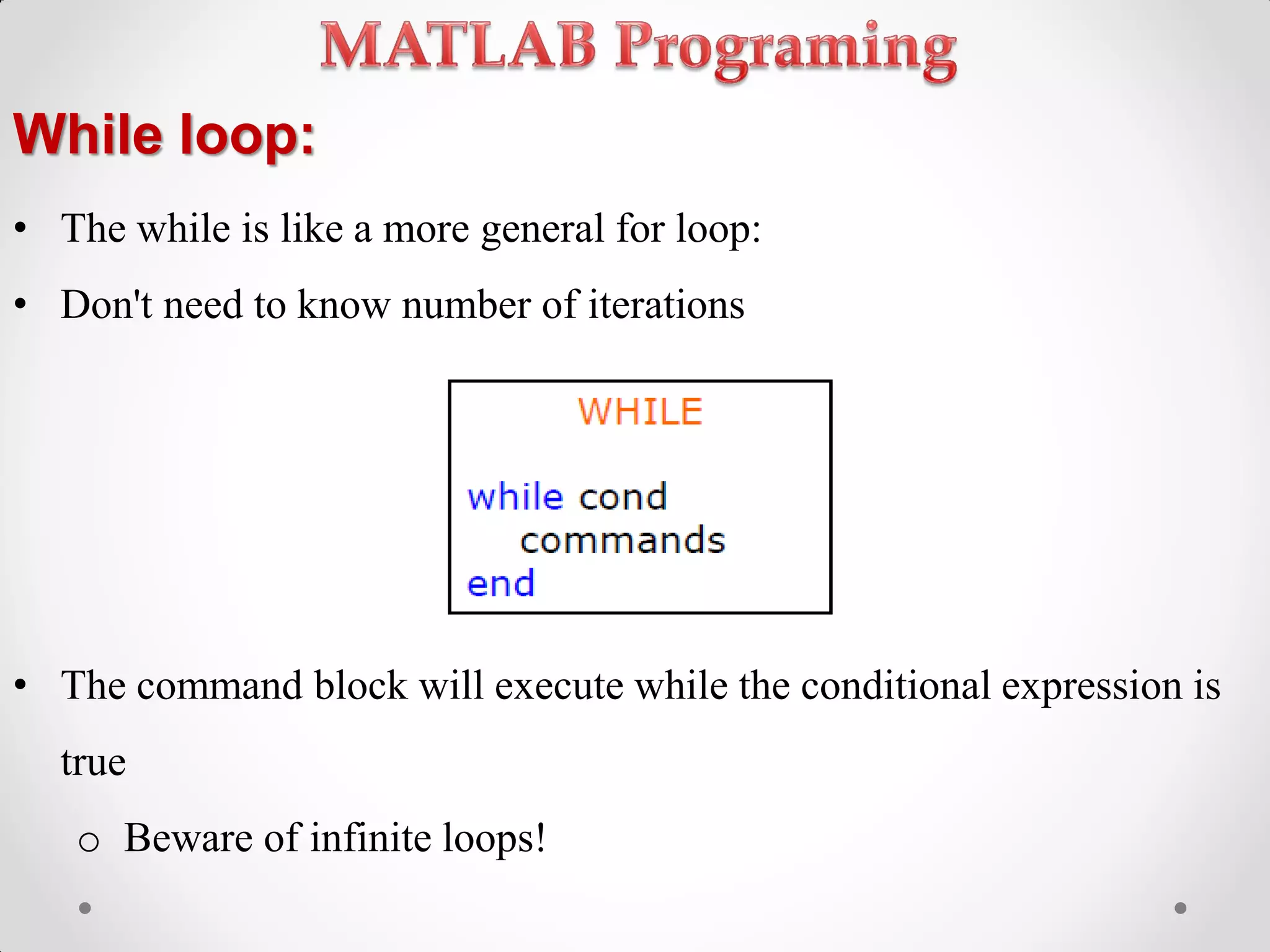
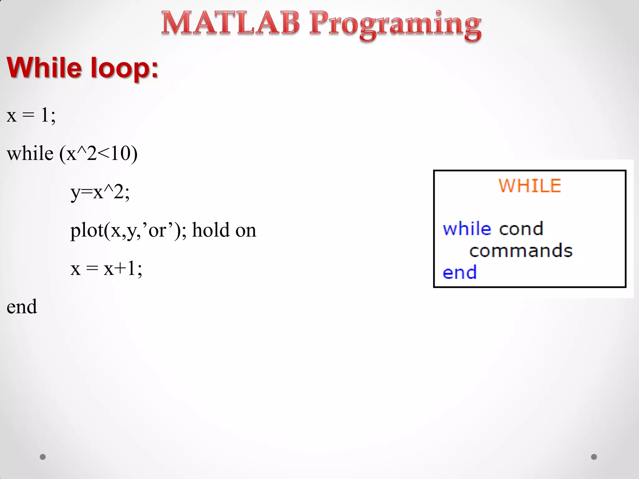
Using for loops and while loops to perform repetitive tasks.
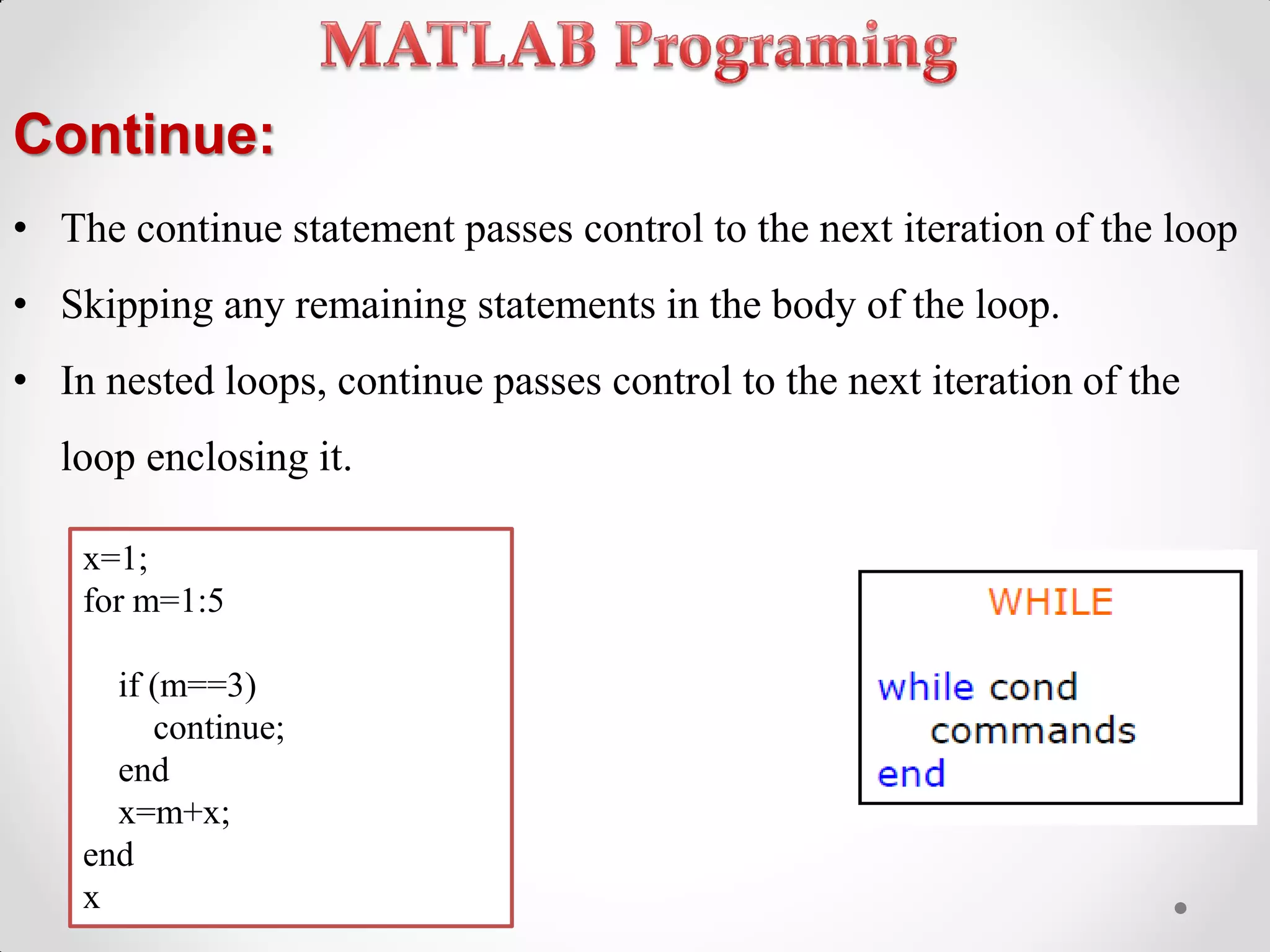
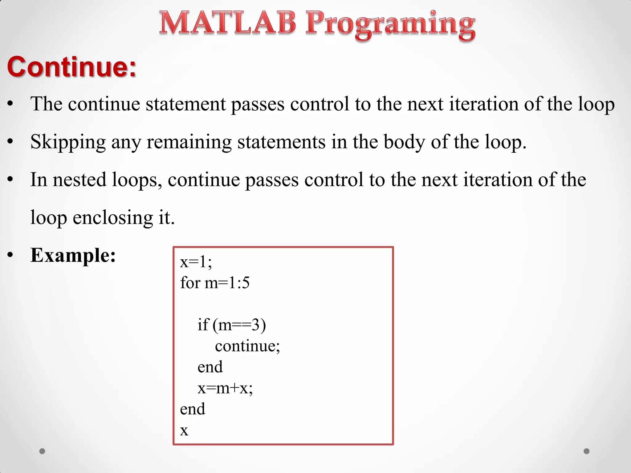
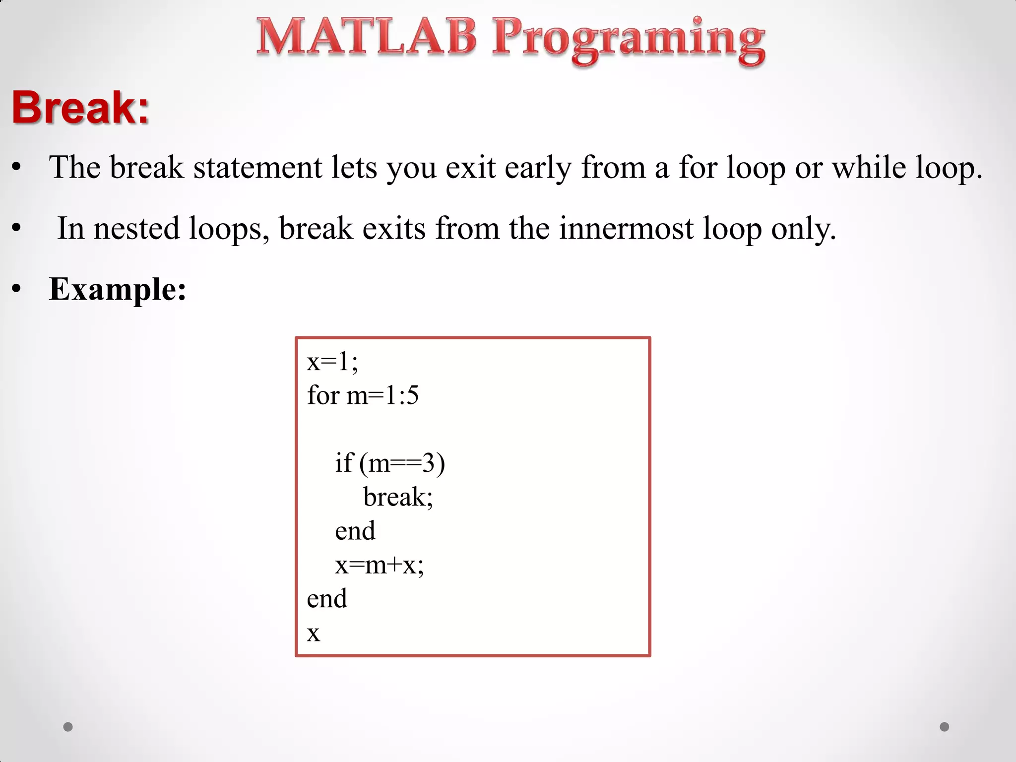
Control flow within loops using continue and break statements.
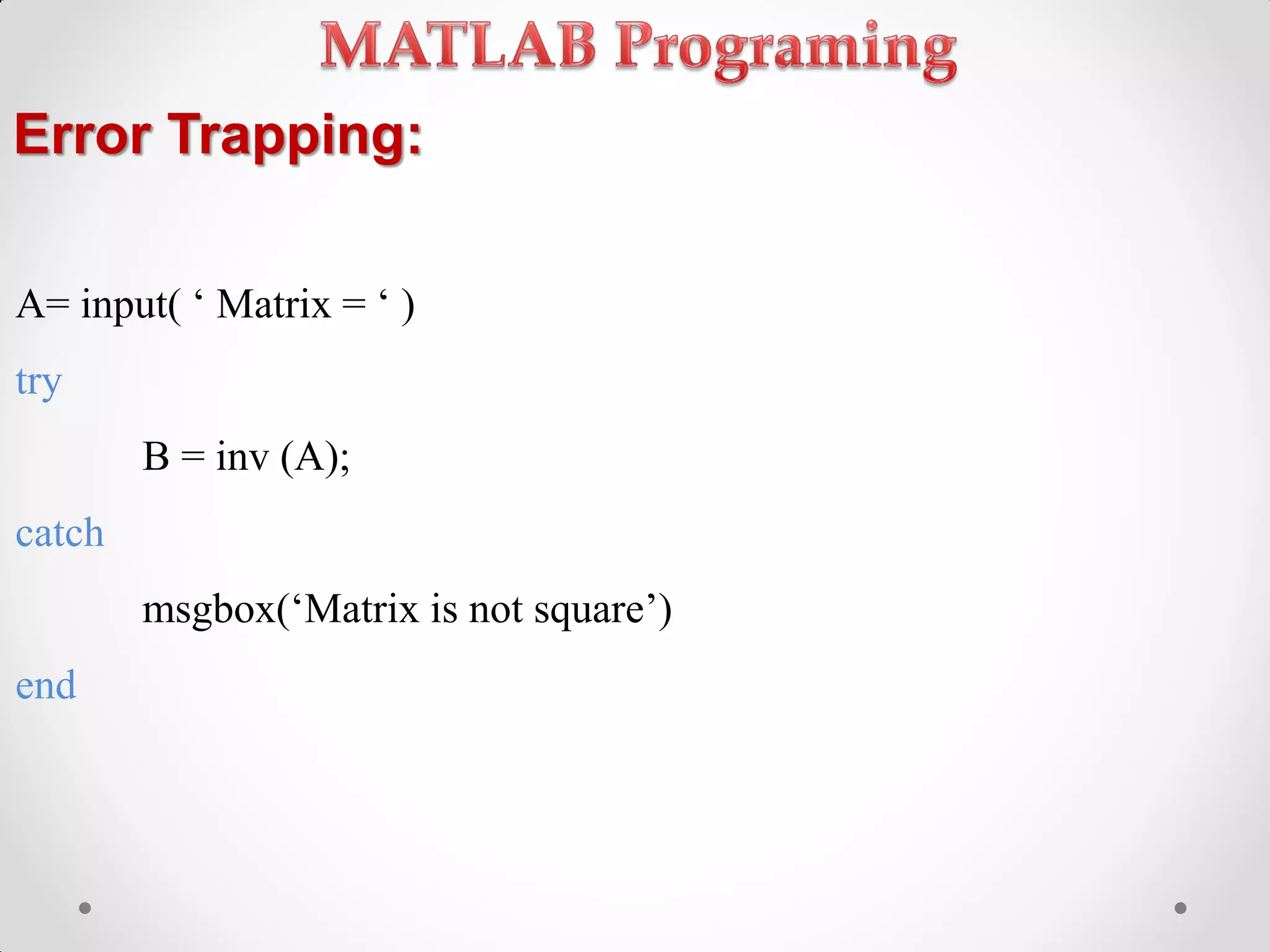
Basic error handling using try-catch for matrix operations.
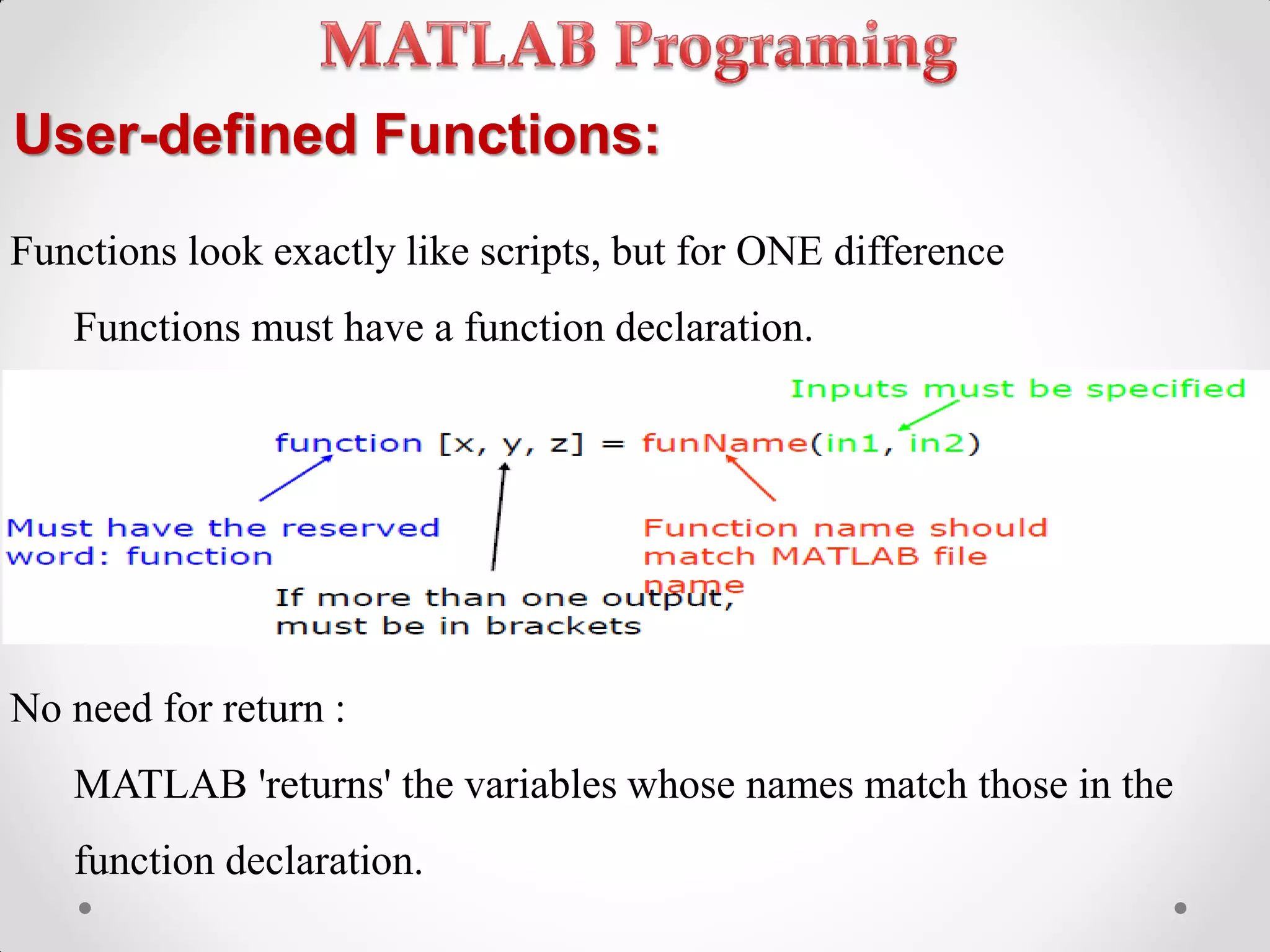
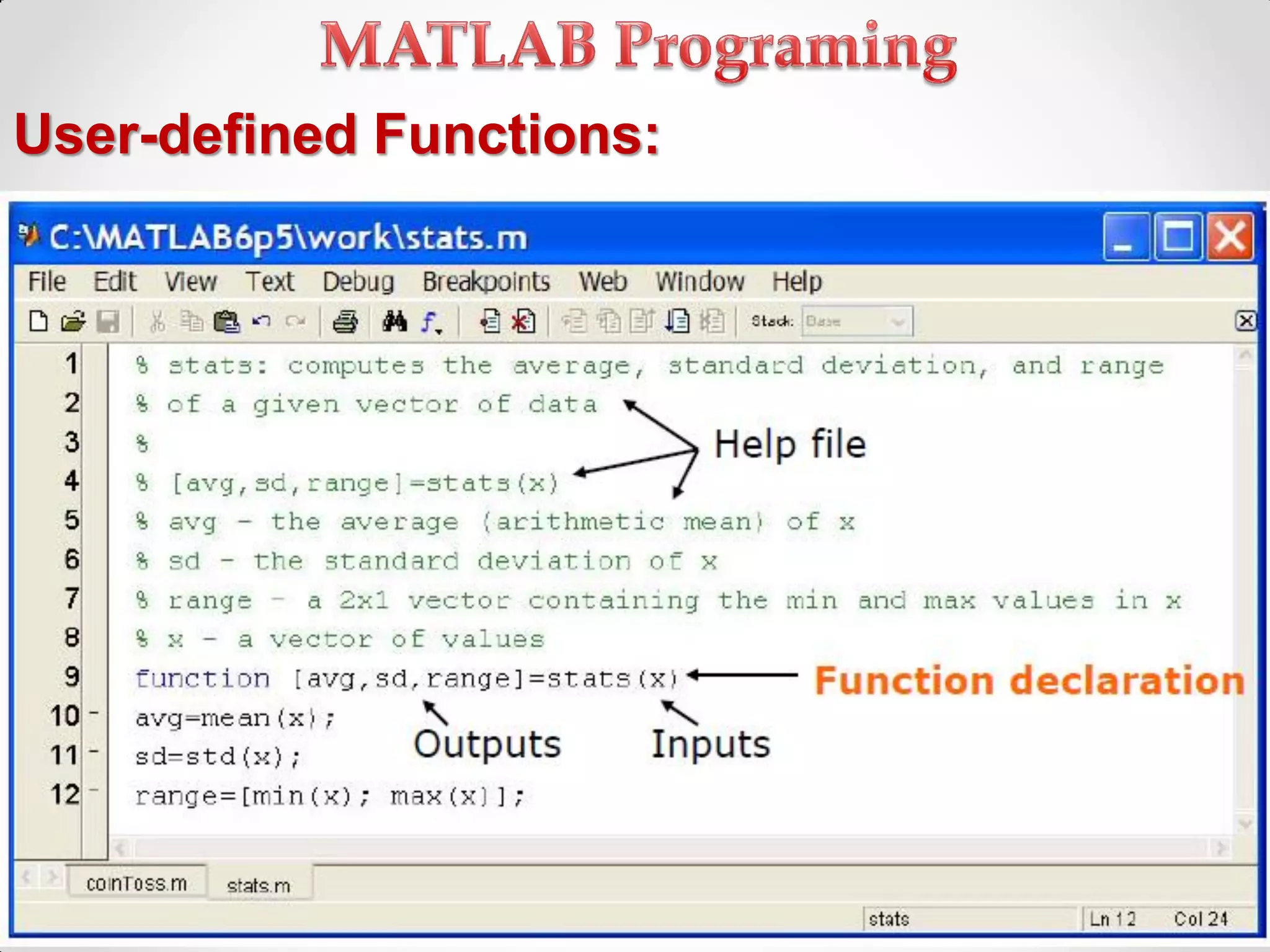
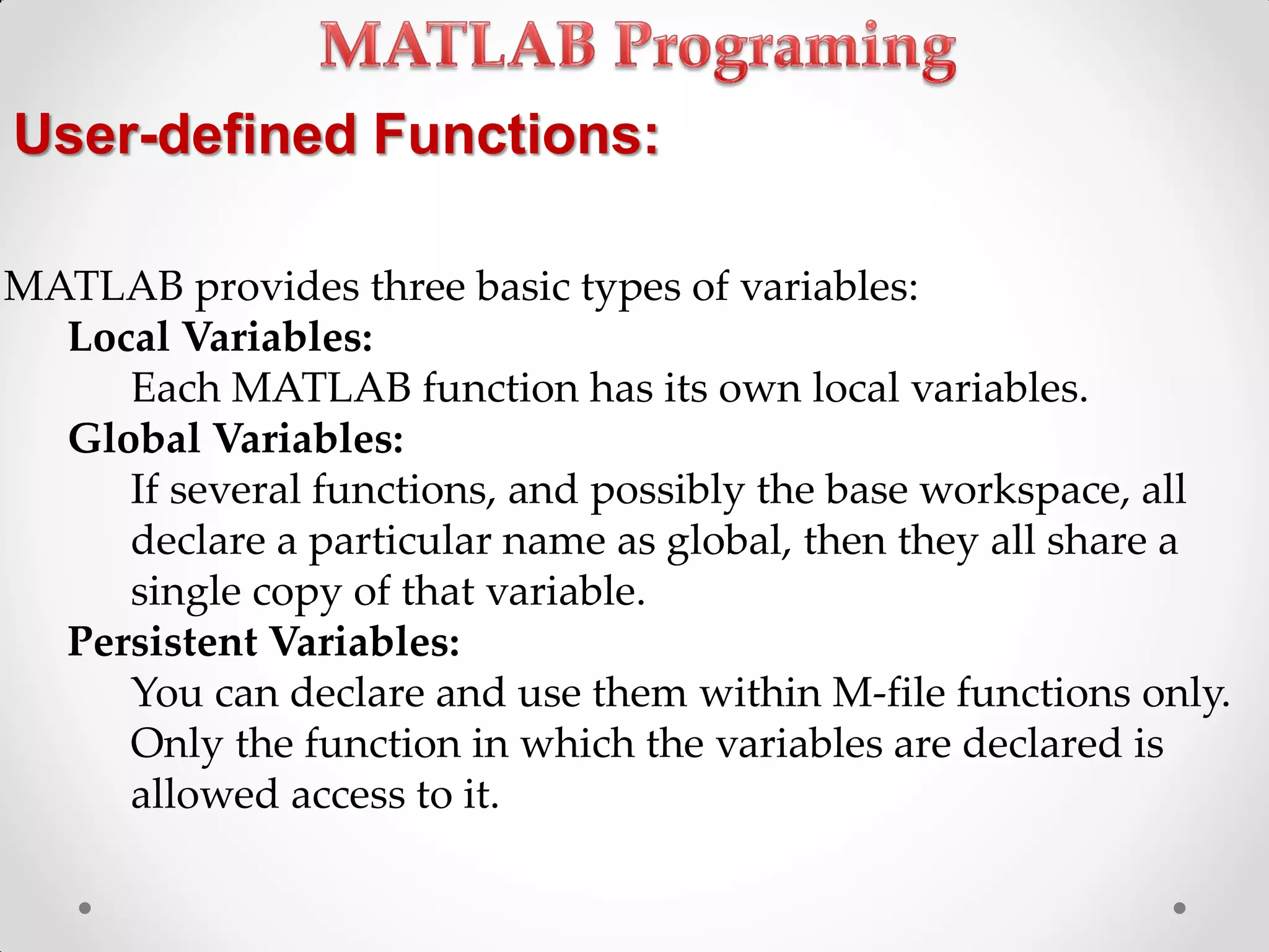
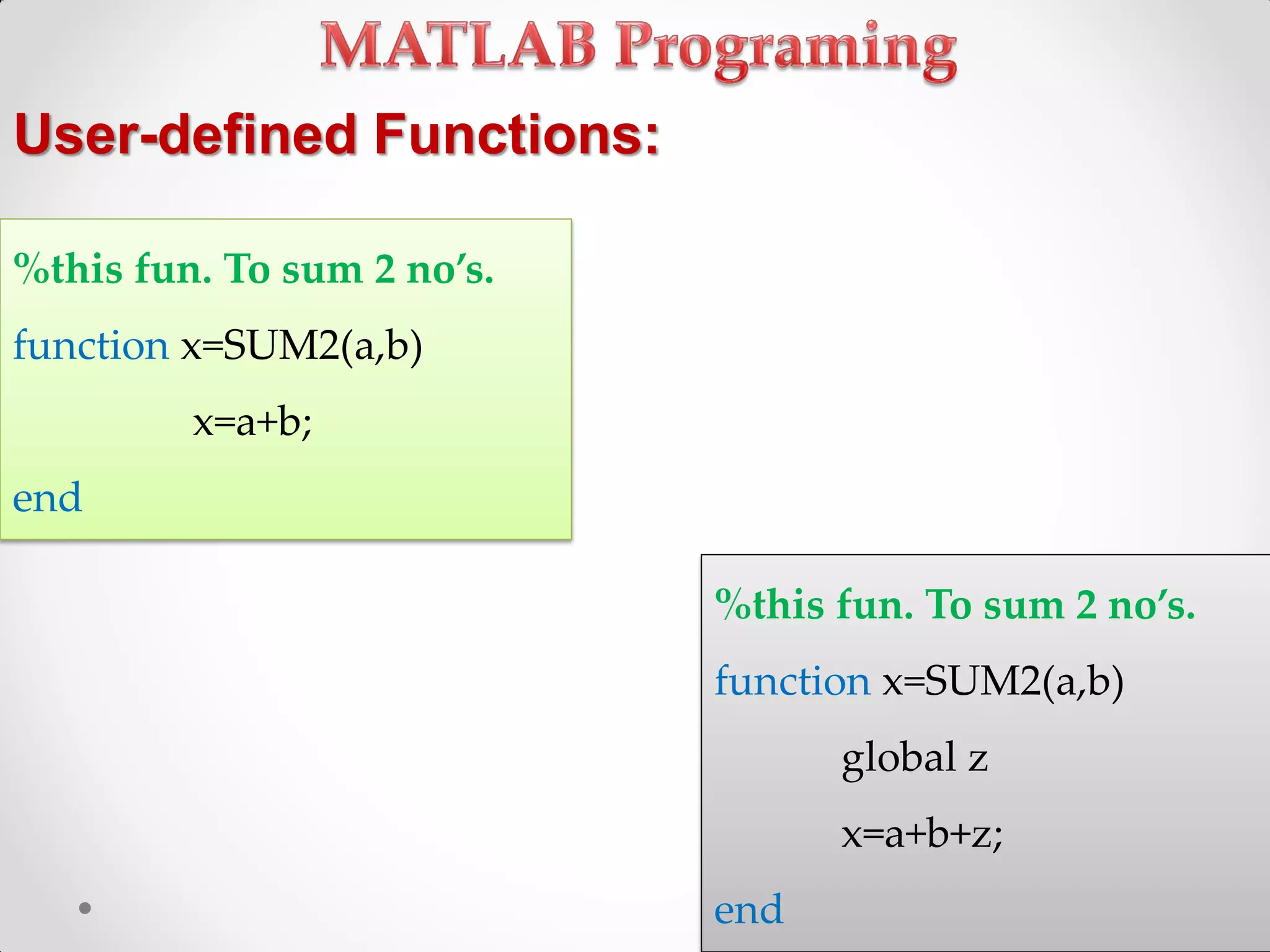
Defining user functions, variable types, and scope of variables in MATLAB.
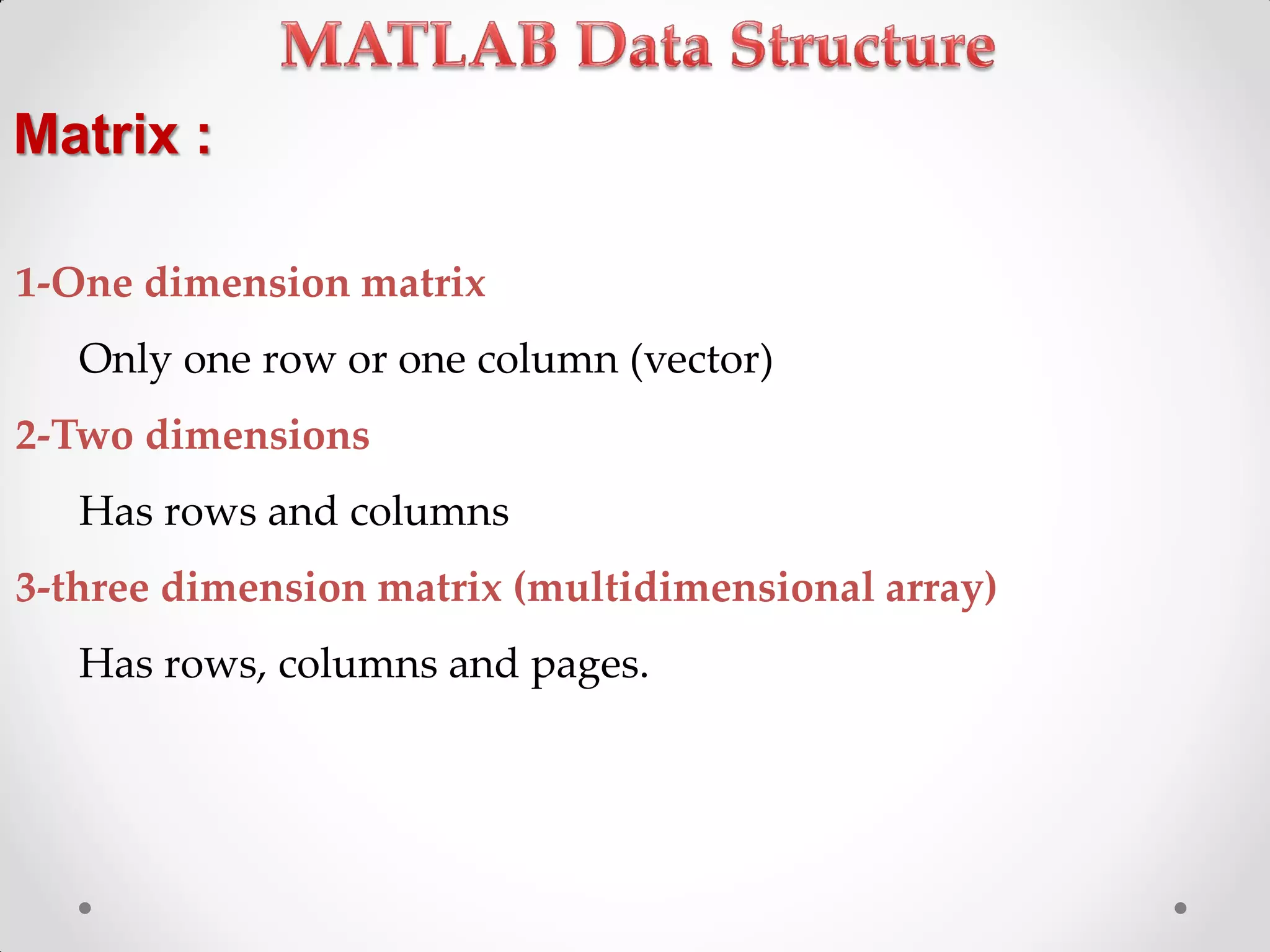
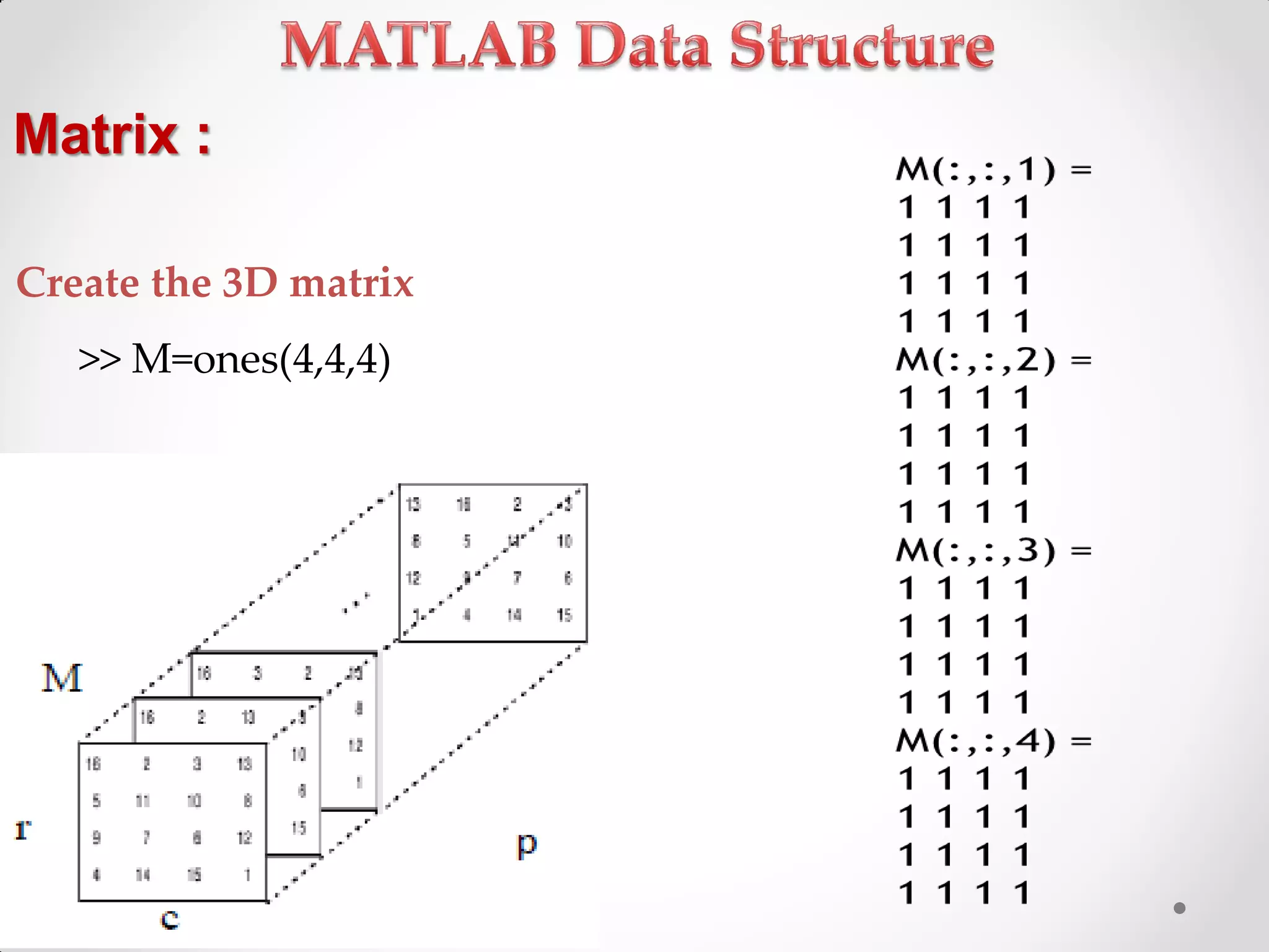
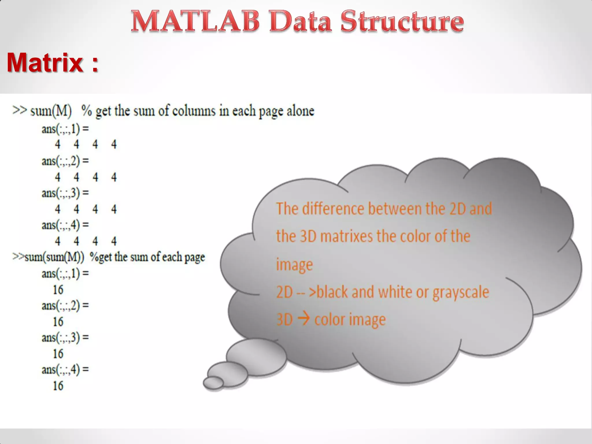
Overview of matrix types and creating multidimensional matrices.
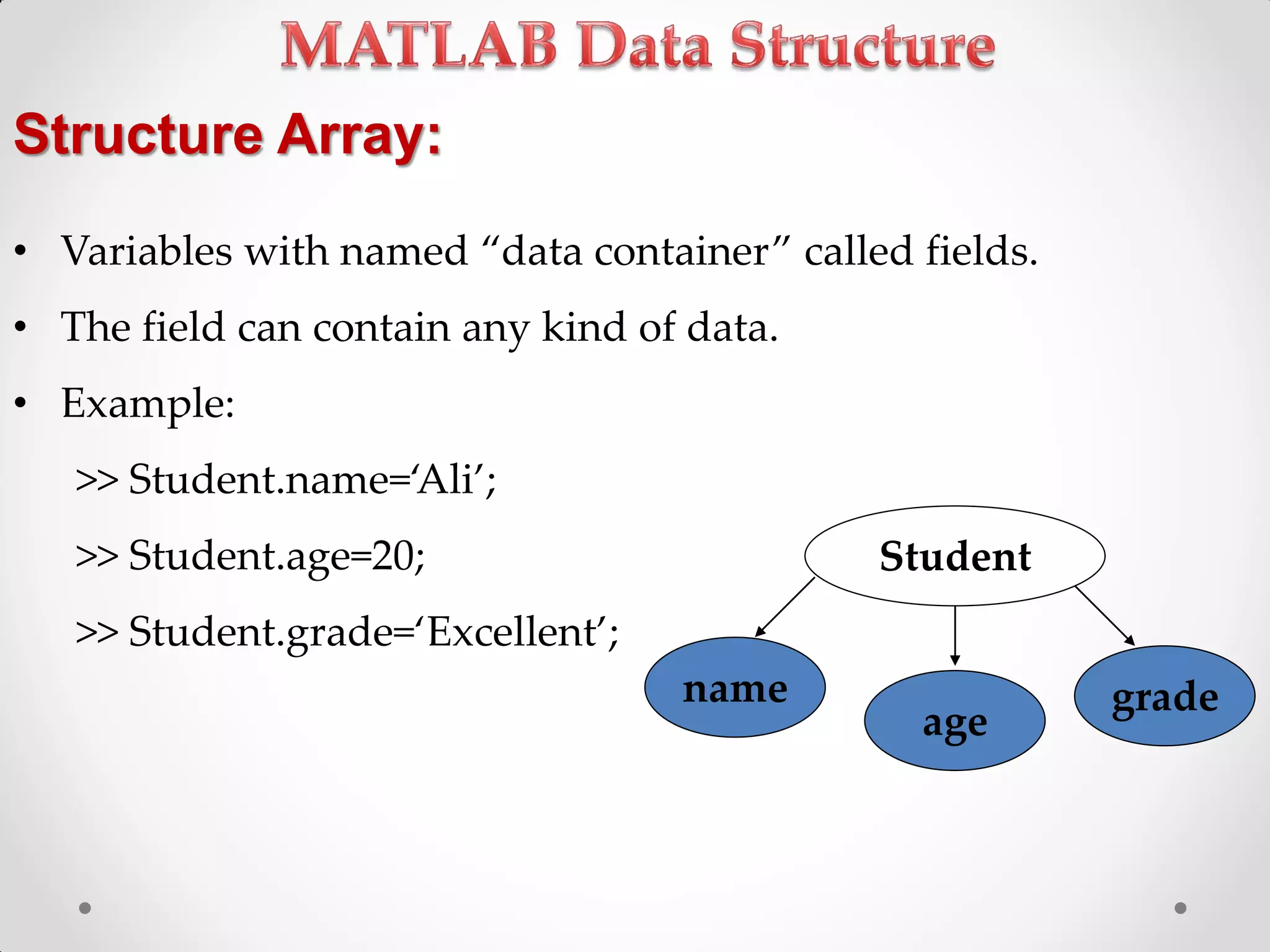
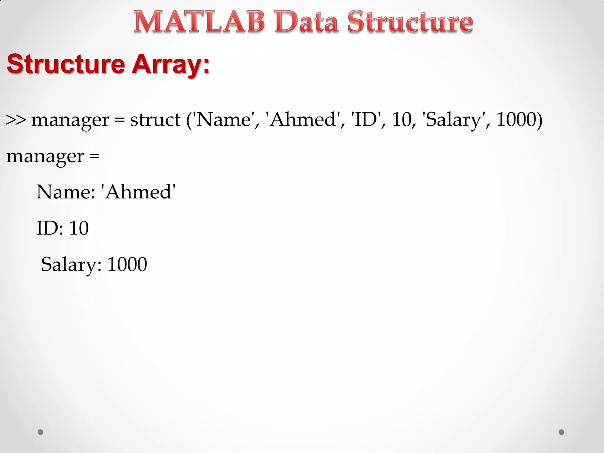
Understanding cell arrays and structure arrays to store different data types.
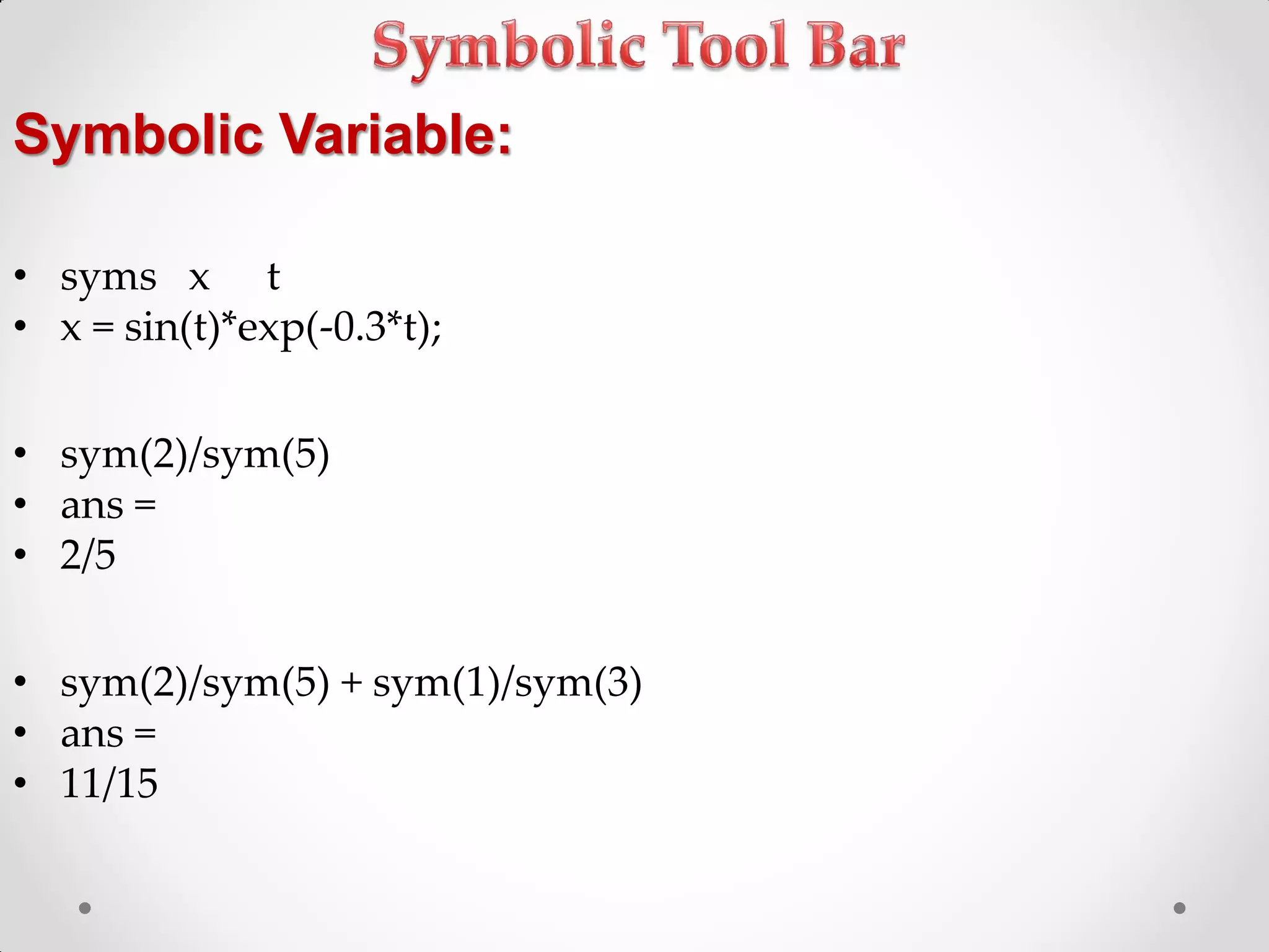
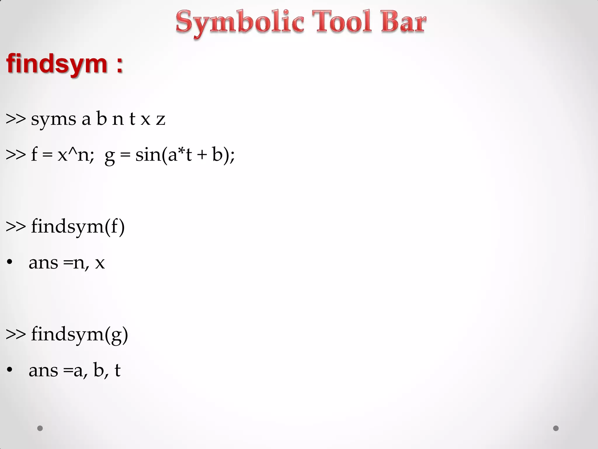
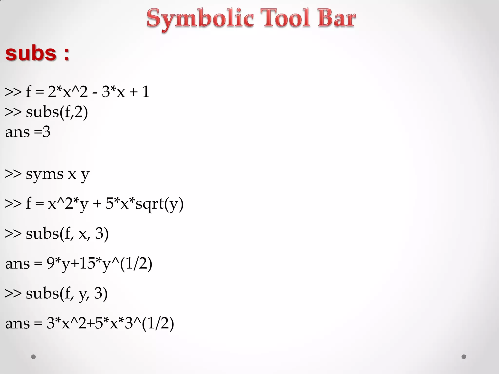
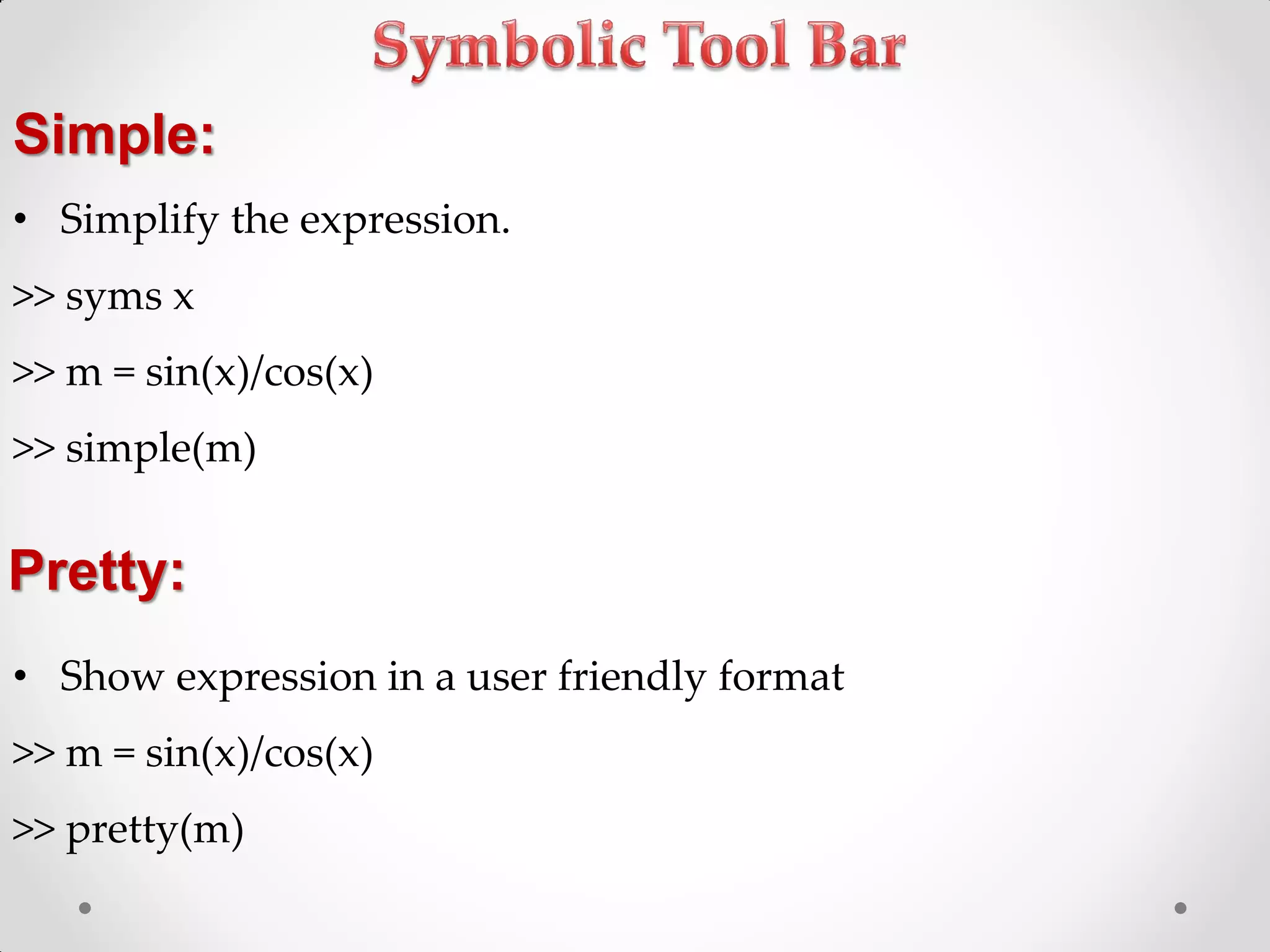
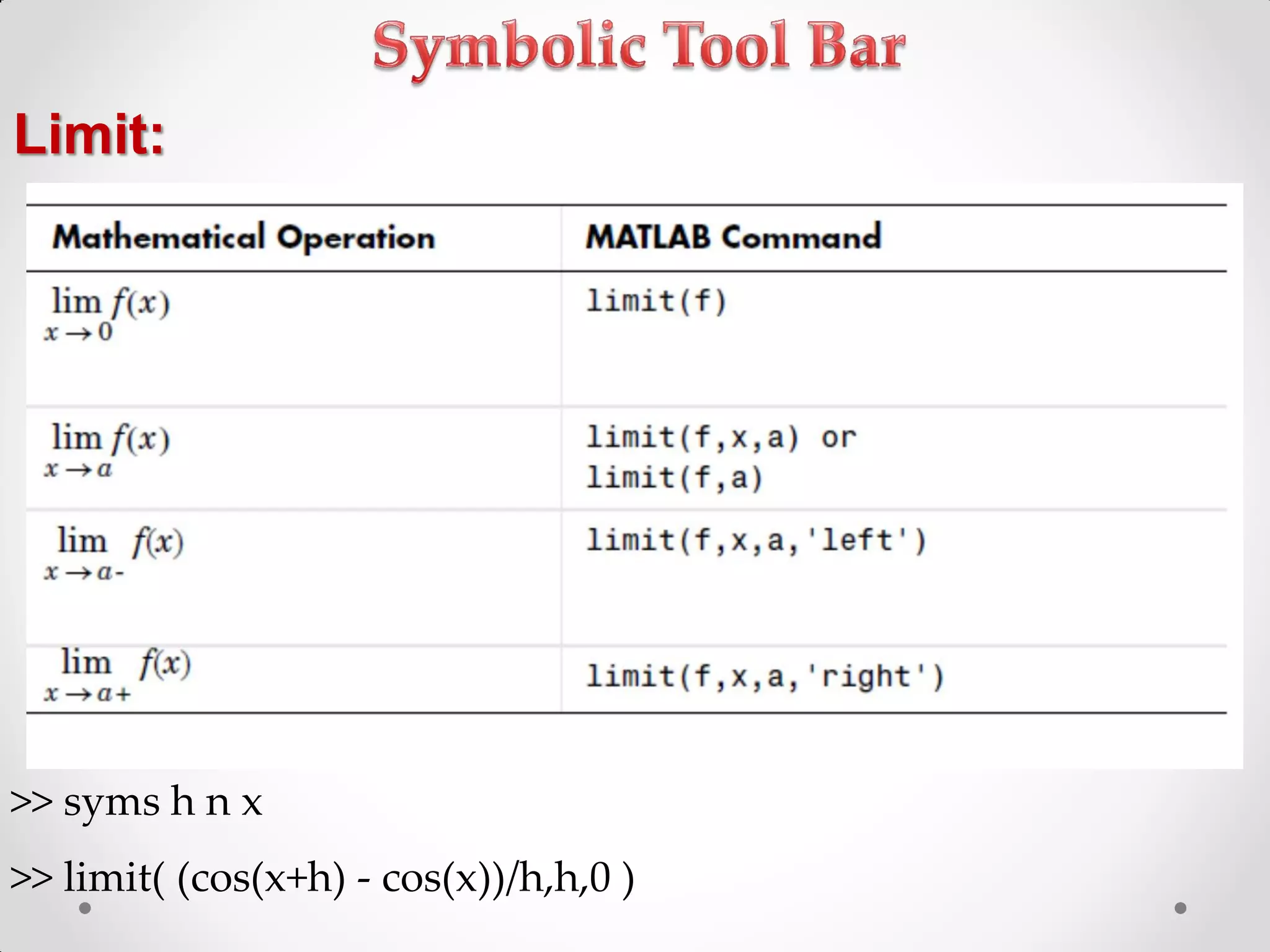
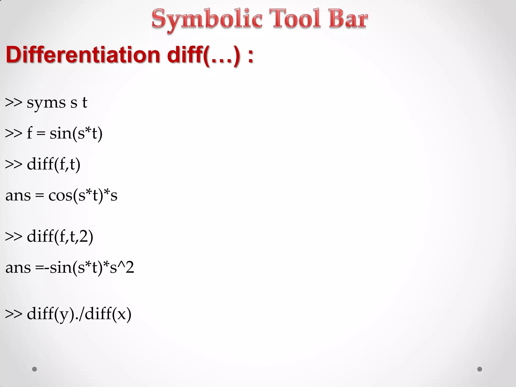
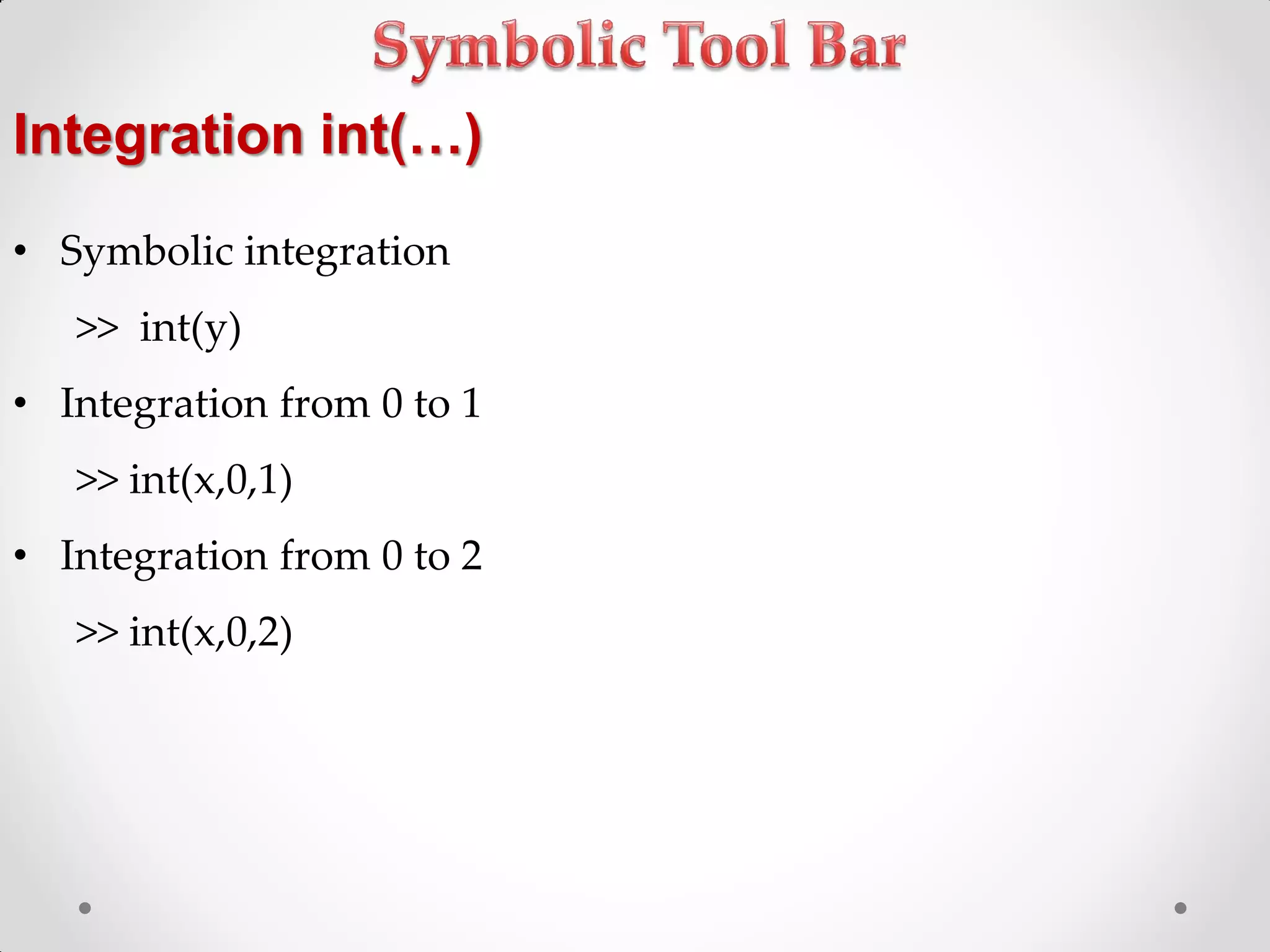
Performing symbolic operations including differentiation, integration, and solving equations.
References for MATLAB resources, courses, and documentation.