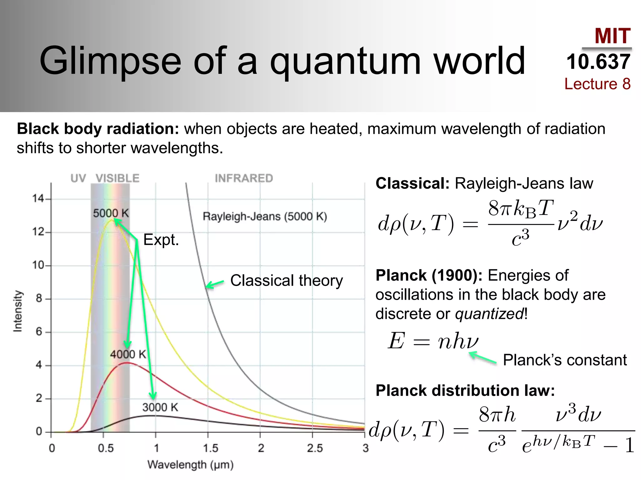
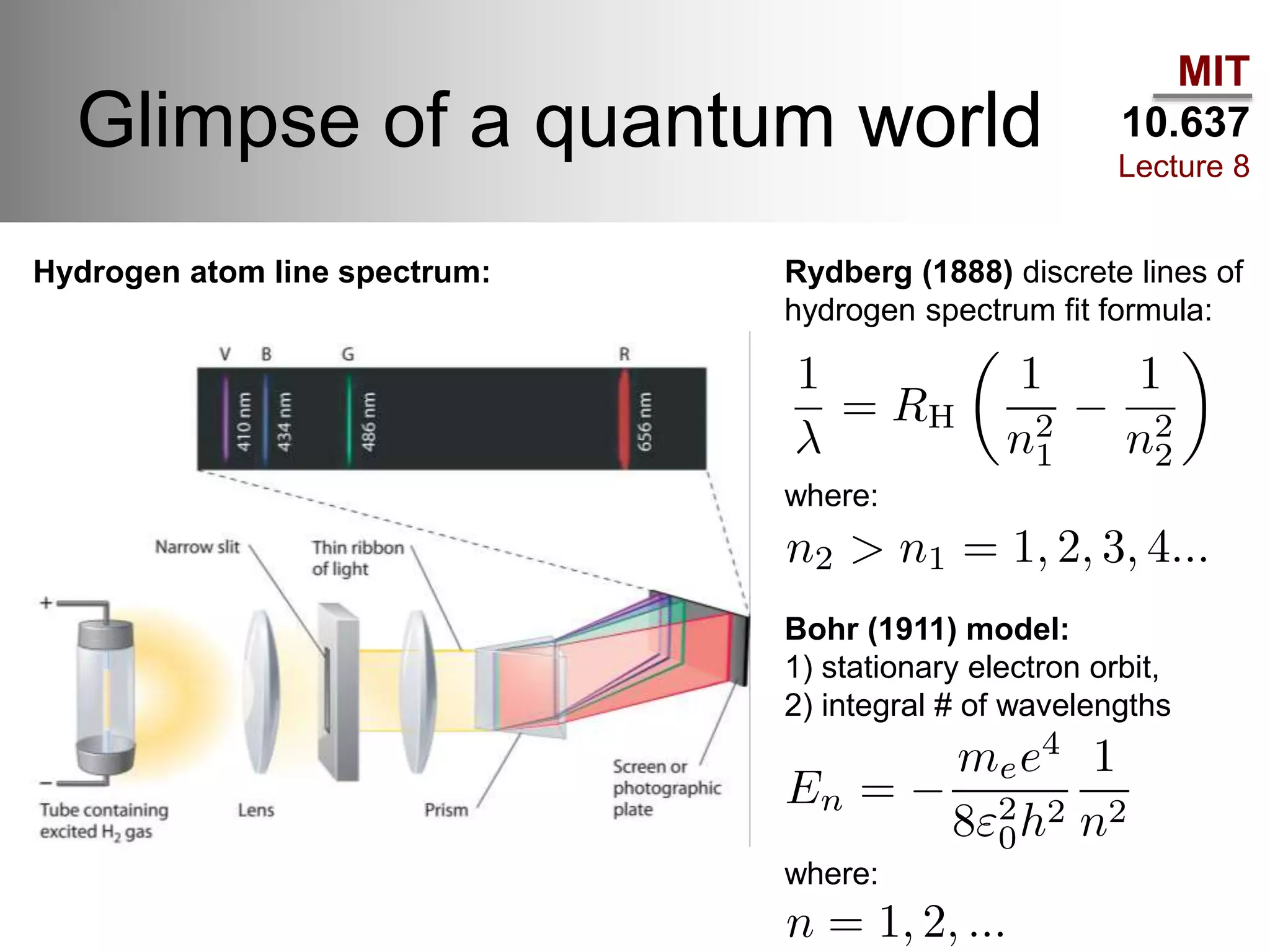
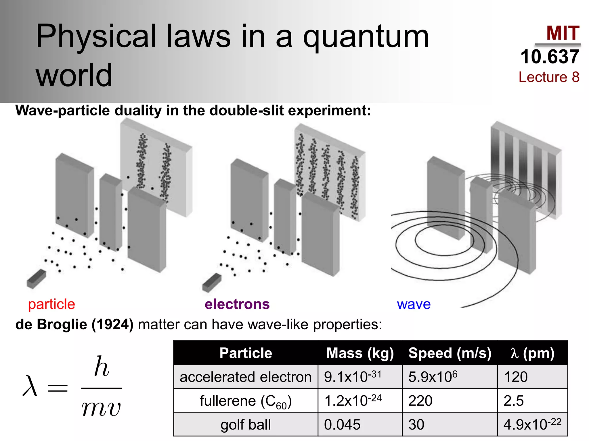
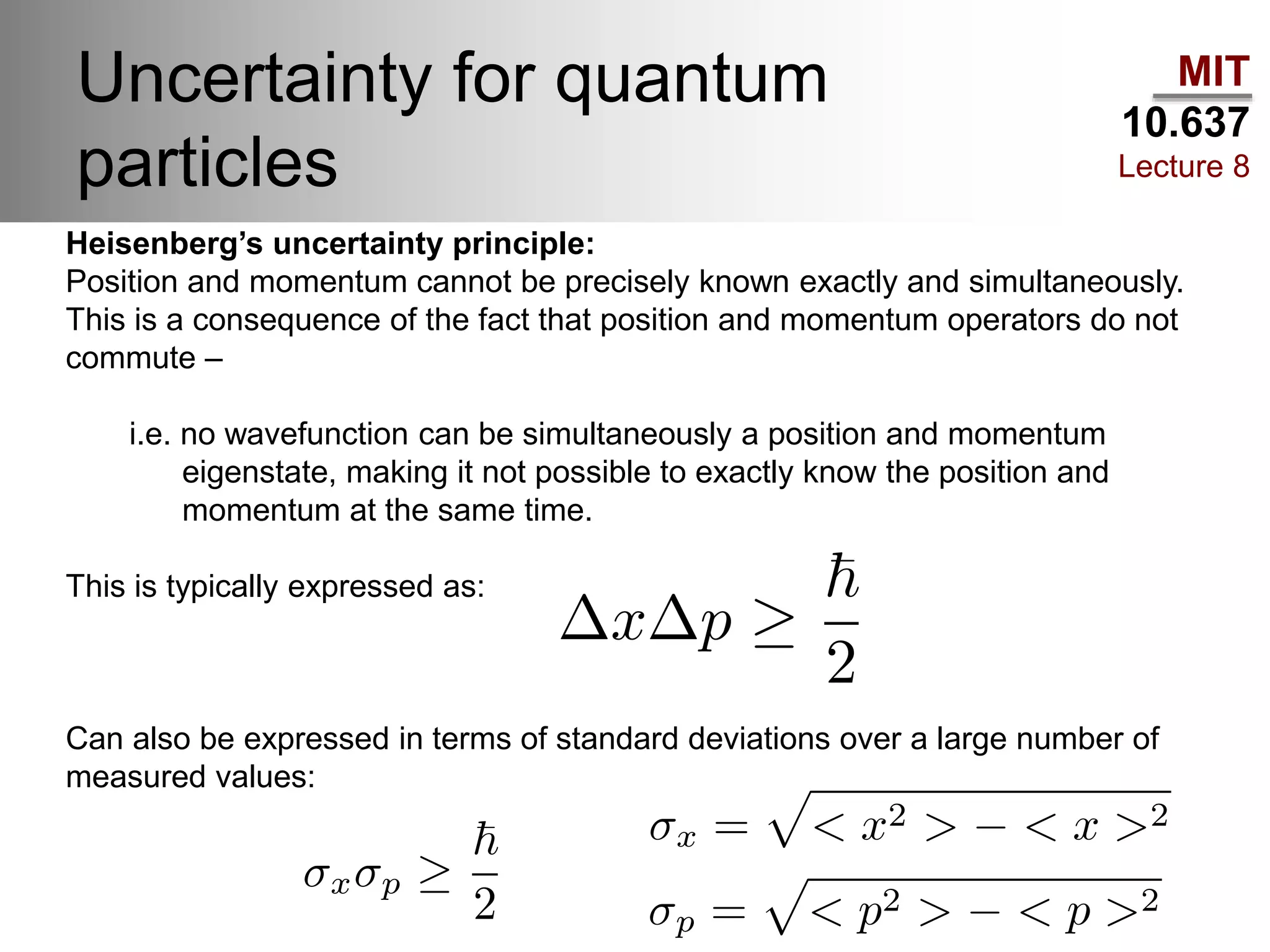
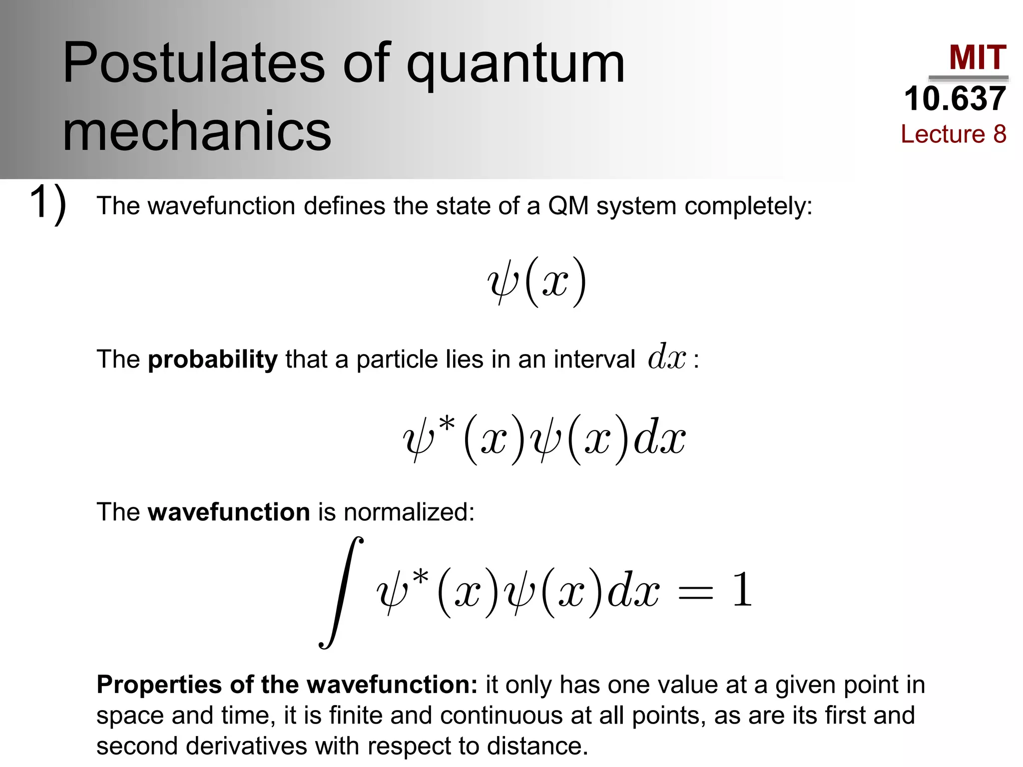
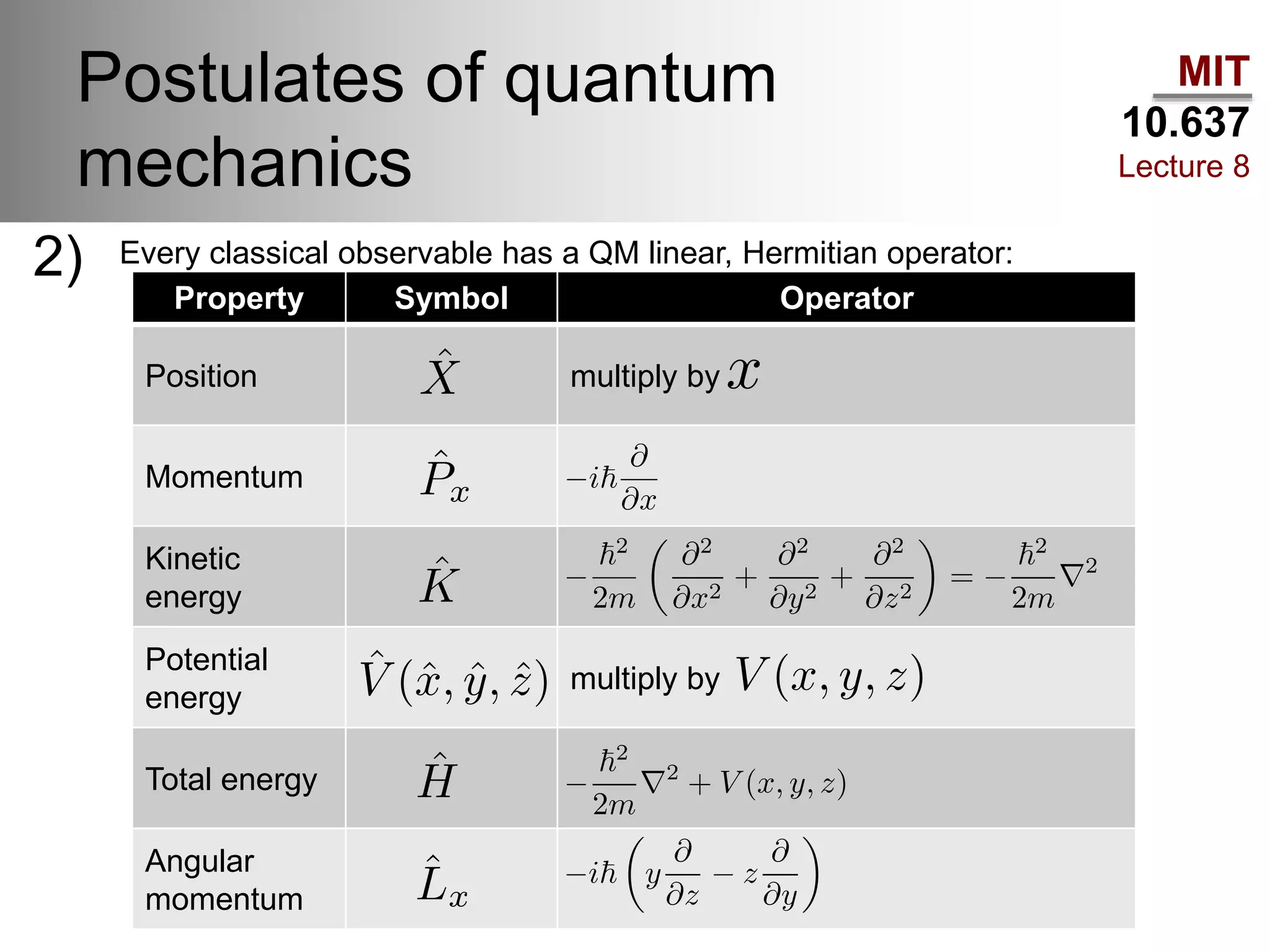
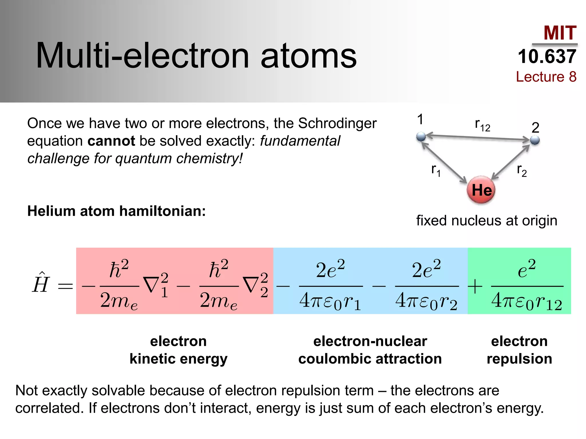
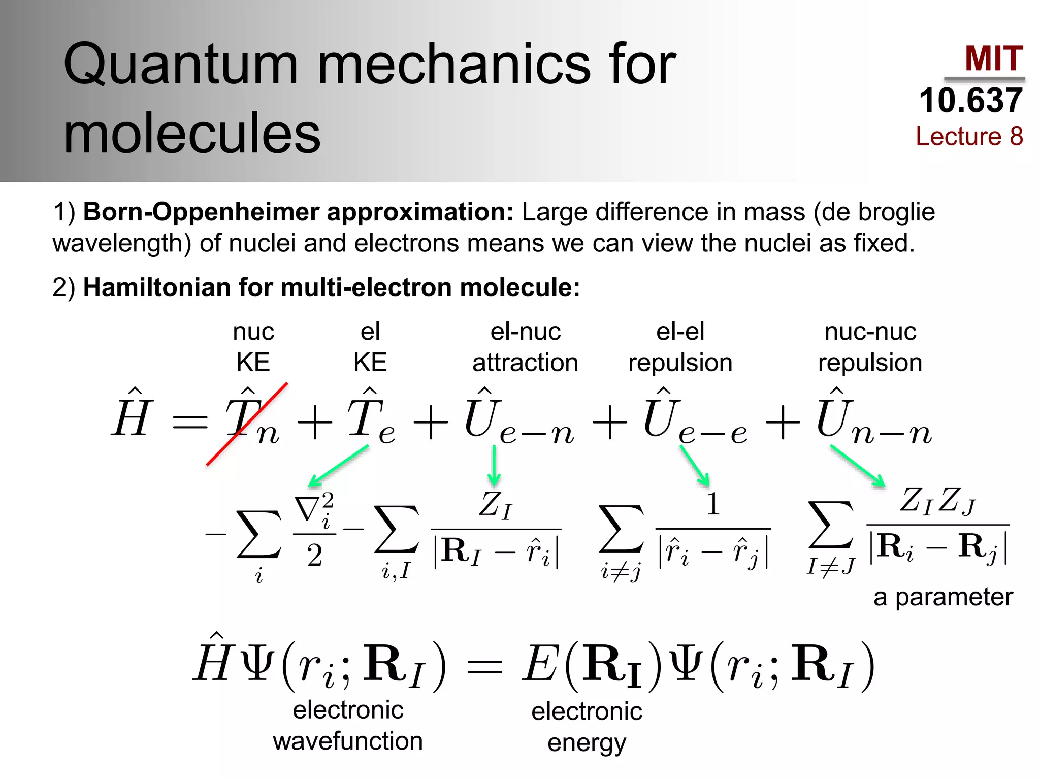
MIT
10.637
Lecture 8
Quantum Mechanics Review
Heather J Kulik
September 30, 2014
MIT
10.637
Lecture 8
A quantum refresher
• This course teaches some concepts that rely
on a basic understanding of quantum
mechanics.
• For a deeper background into quantum
mechanics, consider the courses: 5.73
(Graduate quantum mechanics), 5.61
(undergraduate quantum mechanics).
• Useful textbooks:
– Quantum Chemistry by Ira N. Levine
– Physical Chemistry by McQuarrie & Simon
MIT
10.637
Lecture 8
Glimpse of a quantum world
Black body radiation: when objects are heated, maximum wavelength of radiation
shifts to shorter wavelengths.
Classical theory
Expt.
Classical: Rayleigh-Jeans law
Planck (1900): Energies of
oscillations in the black body are
discrete or quantized!
Planck distribution law:
Planck’s constant
MIT
10.637
Lecture 8
Glimpse of a quantum world
Hydrogen atom line spectrum: Rydberg (1888) discrete lines of
hydrogen spectrum fit formula:
where:
Bohr (1911) model:
1) stationary electron orbit,
2) integral # of wavelengths
where:
MIT
10.637
Lecture 8
Physical laws in a quantum
world
Wave-particle duality in the double-slit experiment:
particle waveelectrons
de Broglie (1924) matter can have wave-like properties:
Particle Mass (kg) Speed (m/s) l (pm)
accelerated electron 9.1x10⁻³¹ 5.9x10⁶ 120
fullerene (C60) 1.2x10⁻²⁴ 220 2.5
golf ball 0.045 30 4.9x10⁻²²
MIT
10.637
Lecture 8
Uncertainty for quantum
particles
Heisenberg’s uncertainty principle:
Position and momentum cannot be precisely known exactly and simultaneously.
This is a consequence of the fact that position and momentum operators do not
commute –
i.e. no wavefunction can be simultaneously a position and momentum
eigenstate, making it not possible to exactly know the position and
momentum at the same time.
This is typically expressed as:
Can also be expressed in terms of standard deviations over a large number of
measured values:
MIT
10.637
Lecture 8
Postulates of quantum
mechanics
The wavefunction defines the state of a QM system completely:
The probability that a particle lies in an interval :
The wavefunction is normalized:
1)
Properties of the wavefunction: it only has one value at a given point in
space and time, it is finite and continuous at all points, as are its first and
second derivatives with respect to distance.
MIT
10.637
Lecture 8
Postulates of quantum
mechanics
2) Every classical observable has a QM linear, Hermitian operator:
Property Symbol Operator
Position multiply by
Momentum
Kinetic
energy
Potential
energy
multiply by
Total energy
Angular
momentum
MIT
10.637
Lecture 8
Operators in other coordinates
Kinetic energy in spherical coordinates:
Angular momentum operators in spherical coordinates:
Combined:
MIT
10.637
Lecture 8
Postulates of quantum
mechanics
3) Observables associated with an operator are eigenvalues of the wavefunction.
4) The average value of an observable is defined as:
The time-independent Schrödinger equation is a special case:
MIT
10.637
Lecture 8
Postulates of quantum
mechanics
5) The wavefunction is solution to the time-dependent Schrödinger equation:
Typically, we can separate the spatial and temporal:
Most wavefunctions of interest are stationary-state solutions:
In this course we focus only on solving the time-independent equation:
MIT
10.637
Lecture 8
A note about notation
complex
conjugate
Dirac or “bra-ket” notation is a useful representation for QM equations:
bra ket
Useful relations Schrödinger equation
TDSE:
TISE:
MIT
10.637
Lecture 8
Properties of operators
Here are some rules for operator algebra:
1) If then
2)
3)
4) Operators corresponding to physical quantities are linear:
5) and Hermitian:
MIT
10.637
Lecture 8
Commuting operators
Two operators commute if their order of application does not change the result
(i.e. they share common eigenfunctions):
Using another notation, we can say this as:
Examples of commuting operators:
Total angular momentum and components commute.
But the components don’t commute with each other.
MIT
10.637
Lecture 8
A free particle
The simplest Schrodinger equation to solve is for the free particle in one
dimension.
The Hamiltonian is simply the kinetic energy operator:
The Schrodinger equation: Rearranged:
Solutions to this simple differential equation:
where
MIT
10.637
Lecture 8
Particle in an infinite well
Particle in a 1D infinite well with boundary conditions:
For 0 ≤ x ≤ a, TISE (same as the free particle):0 x a
8
8
with:
Wavefunction must go to zero outside of the box because the potential is
infinite there. This sets boundary conditions on the wavefunction:
MIT
10.637
Lecture 8
Particle in an infinite well
Solutions for this ODE:
A=0
for
True if:
n = 1, 2, …
MIT
10.637
Lecture 8
Particle in an infinite well
Second boundary condition sets constraint:
Energy levels are quantized! Higher solutions have nodes.
Can rearrange to get energy, even the lowest solution has
some kinetic energy (zero point energy):
From normalization, we obtain the wavefunction:
n = 1, 2, …
MIT
10.637
Lecture 8
Particle in a 3D box
0 x a
0zc
This is an extension of the infinite well problem,
where now the Hamiltonian is:
It can be shown that separation of variables can be carried out. That is the
wavefunction can be written as a product of functions that each depend only on one
coordinate (this is relevant for later):
The solution looks just like a product of the 1D solutions:
Energy levels can be
degenerate (multiple
states) for cubic boxes.
MIT
10.637
Lecture 8
Moving on…
• We won’t solve every Hamiltonian.
• What you should understand so far is that:
– Solving the Schrodinger equation gives us
eigenvalues (energies) and eigenfunctions
(wavefunctions).
– Solutions to this quantum mechanical master
equation are often quantized.
– The lowest energy solution will have non-zero
kinetic energy: zero point energy, Heisenberg
uncertainty principle.
– There may be degeneracy in the energy levels.
– We are just solving differential equations.
MIT
10.637
Lecture 8
Hydrogen atom
+
We use a reference frame where the nucleus is fixed:
proton
Coulomb
potential The potential is simply the Coulomb interaction
between two point charges:
The total Hamiltonian:
The geometry motivates use of spherical coordinates. Recall the Laplacian:
MIT
10.637
Lecture 8
Hydrogen atom
It’s a little too painful to do the full derivation here.
In the spirit of separation of variables, we will treat the three
variables (r, q, f) separately, but they depend on each other
through parameters. We solve the Schrodinger equation
sequentially and replace an operator with the operator’s
eigenvalue.
A general strategy:
1. Start with the f – get eigenvalues and eigenstates of second
derivatives in f.
2. Solve the q part – finding eigenvalues and eigenvectors of
angular momentum operator.
3. Replace operator with eigenvalues so Hamiltonian depends
only on r.
4. Solve the Schrodinger equation in r.
1+2 are the same as solving the quantum rigid rotor.
MIT
10.637
Lecture 8
Rigid rotor
moment of inertia for
linear molecule.
Schrodinger equation in spherical (I is constant):
Group together constants:
Rearrange Schrodinger equation (multiply by sin2q):
terms only contain q terms only contain f
MIT
10.637
Lecture 8
Rigid rotor
The wavefunction must be a product of the independent functions:
And the two sides of the equations should be equal to a constant (arbitrarily set to m2
for now) and the derivatives are no longer partial:
(1)
(2)
Solution to (2) is simple, same form as for free electron:
MIT
10.637
Lecture 8
Rigid rotor
These are associated Legendre polynomials of cosq
Solution to (1) is more challenging and outside of the scope of this review. Solution
introduces a second constant l and m is also referred to as ml:
MIT
10.637
Lecture 8
Rigid rotor
Combined solution with normalization are called spherical harmonics:
These are also referred to by the variable
The energy levels are:
where:
MIT
10.637
Lecture 8
Hydrogen atom
Now, we return to the hydrogen atom, noting that we are working with separation
of variables because the potential is only dependent on r and we can separate the
components of the Laplacian:
Write out a simplified version of the Hamiltonian on this separated wavefunction
and with operators only acting on relevant components of the wavefunction:
MIT
10.637
Lecture 8
Hydrogen atom
We can separate out the one component dependent on f and q from our previous
analysis of the rigid rotor:
So we insert the eigenvalues into Hamiltonian and divide by :
This differential equation can be solved (not shown here) and the resulting
solutions are related to the associated Laguerre polynomials.
MIT
10.637
Lecture 8
Hydrogen atom
associated Laguerre polynomials
Solutions (skipping some steps) and using the definition of the Bohr radius as a
constant:
where: energy levels:
MIT
10.637
Lecture 8
Hydrogen atom
associated Laguerre polynomials
Some example solutions of:
MIT
10.637
Lecture 8
Hydrogen atom
Quantum numbers from gen. chem. directly from solving the hydrogen atom
Hamiltonian:
Real parts of the spherical harmonics in hydrogen atom wavefunction:
Linear combinations of spherical harmonics to produce only real orbitals.
Radial part: Spherical harmonics (rigid rotor solutions):
Principle quantum number
Determines # nodes (n-1)
Azimuthal QN – angular
momenta (s=0,p=1,d=2…)
Magnetic QN –
distinguishes between
wfns of same AM
MIT
10.637
Lecture 8
Hydrogen atom – radial part
MIT
10.637
Lecture 8
Hydrogen atom wavefunction
MIT
10.637
Lecture 8
Multi-electron atoms
Once we have two or more electrons, the Schrodinger
equation cannot be solved exactly: fundamental
challenge for quantum chemistry!
Helium atom hamiltonian:
fixed nucleus at origin
1
2r12
r2r1
He
electron
kinetic energy
electron-nuclear
coulombic attraction
electron
repulsion
Not exactly solvable because of electron repulsion term – the electrons are
correlated. If electrons don’t interact, energy is just sum of each electron’s energy.
MIT
10.637
Lecture 8
Quantum mechanics for
molecules
1) Born-Oppenheimer approximation: Large difference in mass (de broglie
wavelength) of nuclei and electrons means we can view the nuclei as fixed.
2) Hamiltonian for multi-electron molecule:
nuc
KE
el
KE
el-nuc
attraction
el-el
repulsion
nuc-nuc
repulsion
electronic
energy
electronic
wavefunction
a parameter
MIT
10.637
Lecture 8
Where do we go from here?
• Perturbation theory allows us to make a
zeroth order Hamiltonian and then can add in
corrections perturbatively – e.g. Helium using
Hydrogen as initial guess.
• Can use variation theorem to guess the form
of the wavefunction and then iterativey
improve it until the energy is lowered.
• Next classes: quantum chemistry allows us to
approximately solve the Schrodinger
equation.

Lecture7

  • 1.
    MIT 10.637 Lecture 8 Quantum MechanicsReview Heather J Kulik September 30, 2014
  • 2.
    MIT 10.637 Lecture 8 A quantumrefresher • This course teaches some concepts that rely on a basic understanding of quantum mechanics. • For a deeper background into quantum mechanics, consider the courses: 5.73 (Graduate quantum mechanics), 5.61 (undergraduate quantum mechanics). • Useful textbooks: – Quantum Chemistry by Ira N. Levine – Physical Chemistry by McQuarrie & Simon
  • 3.
    MIT 10.637 Lecture 8 Glimpse ofa quantum world Black body radiation: when objects are heated, maximum wavelength of radiation shifts to shorter wavelengths. Classical theory Expt. Classical: Rayleigh-Jeans law Planck (1900): Energies of oscillations in the black body are discrete or quantized! Planck distribution law: Planck’s constant
  • 4.
    MIT 10.637 Lecture 8 Glimpse ofa quantum world Hydrogen atom line spectrum: Rydberg (1888) discrete lines of hydrogen spectrum fit formula: where: Bohr (1911) model: 1) stationary electron orbit, 2) integral # of wavelengths where:
  • 5.
    MIT 10.637 Lecture 8 Physical lawsin a quantum world Wave-particle duality in the double-slit experiment: particle waveelectrons de Broglie (1924) matter can have wave-like properties: Particle Mass (kg) Speed (m/s) l (pm) accelerated electron 9.1x10⁻³¹ 5.9x10⁶ 120 fullerene (C60) 1.2x10⁻²⁴ 220 2.5 golf ball 0.045 30 4.9x10⁻²²
  • 6.
    MIT 10.637 Lecture 8 Uncertainty forquantum particles Heisenberg’s uncertainty principle: Position and momentum cannot be precisely known exactly and simultaneously. This is a consequence of the fact that position and momentum operators do not commute – i.e. no wavefunction can be simultaneously a position and momentum eigenstate, making it not possible to exactly know the position and momentum at the same time. This is typically expressed as: Can also be expressed in terms of standard deviations over a large number of measured values:
  • 7.
    MIT 10.637 Lecture 8 Postulates ofquantum mechanics The wavefunction defines the state of a QM system completely: The probability that a particle lies in an interval : The wavefunction is normalized: 1) Properties of the wavefunction: it only has one value at a given point in space and time, it is finite and continuous at all points, as are its first and second derivatives with respect to distance.
  • 8.
    MIT 10.637 Lecture 8 Postulates ofquantum mechanics 2) Every classical observable has a QM linear, Hermitian operator: Property Symbol Operator Position multiply by Momentum Kinetic energy Potential energy multiply by Total energy Angular momentum
  • 9.
    MIT 10.637 Lecture 8 Operators inother coordinates Kinetic energy in spherical coordinates: Angular momentum operators in spherical coordinates: Combined:
  • 10.
    MIT 10.637 Lecture 8 Postulates ofquantum mechanics 3) Observables associated with an operator are eigenvalues of the wavefunction. 4) The average value of an observable is defined as: The time-independent Schrödinger equation is a special case:
  • 11.
    MIT 10.637 Lecture 8 Postulates ofquantum mechanics 5) The wavefunction is solution to the time-dependent Schrödinger equation: Typically, we can separate the spatial and temporal: Most wavefunctions of interest are stationary-state solutions: In this course we focus only on solving the time-independent equation:
  • 12.
    MIT 10.637 Lecture 8 A noteabout notation complex conjugate Dirac or “bra-ket” notation is a useful representation for QM equations: bra ket Useful relations Schrödinger equation TDSE: TISE:
  • 13.
    MIT 10.637 Lecture 8 Properties ofoperators Here are some rules for operator algebra: 1) If then 2) 3) 4) Operators corresponding to physical quantities are linear: 5) and Hermitian:
  • 14.
    MIT 10.637 Lecture 8 Commuting operators Twooperators commute if their order of application does not change the result (i.e. they share common eigenfunctions): Using another notation, we can say this as: Examples of commuting operators: Total angular momentum and components commute. But the components don’t commute with each other.
  • 15.
    MIT 10.637 Lecture 8 A freeparticle The simplest Schrodinger equation to solve is for the free particle in one dimension. The Hamiltonian is simply the kinetic energy operator: The Schrodinger equation: Rearranged: Solutions to this simple differential equation: where
  • 16.
    MIT 10.637 Lecture 8 Particle inan infinite well Particle in a 1D infinite well with boundary conditions: For 0 ≤ x ≤ a, TISE (same as the free particle):0 x a 8 8 with: Wavefunction must go to zero outside of the box because the potential is infinite there. This sets boundary conditions on the wavefunction:
  • 17.
    MIT 10.637 Lecture 8 Particle inan infinite well Solutions for this ODE: A=0 for True if: n = 1, 2, …
  • 18.
    MIT 10.637 Lecture 8 Particle inan infinite well Second boundary condition sets constraint: Energy levels are quantized! Higher solutions have nodes. Can rearrange to get energy, even the lowest solution has some kinetic energy (zero point energy): From normalization, we obtain the wavefunction: n = 1, 2, …
  • 19.
    MIT 10.637 Lecture 8 Particle ina 3D box 0 x a 0zc This is an extension of the infinite well problem, where now the Hamiltonian is: It can be shown that separation of variables can be carried out. That is the wavefunction can be written as a product of functions that each depend only on one coordinate (this is relevant for later): The solution looks just like a product of the 1D solutions: Energy levels can be degenerate (multiple states) for cubic boxes.
  • 20.
    MIT 10.637 Lecture 8 Moving on… •We won’t solve every Hamiltonian. • What you should understand so far is that: – Solving the Schrodinger equation gives us eigenvalues (energies) and eigenfunctions (wavefunctions). – Solutions to this quantum mechanical master equation are often quantized. – The lowest energy solution will have non-zero kinetic energy: zero point energy, Heisenberg uncertainty principle. – There may be degeneracy in the energy levels. – We are just solving differential equations.
  • 21.
    MIT 10.637 Lecture 8 Hydrogen atom + Weuse a reference frame where the nucleus is fixed: proton Coulomb potential The potential is simply the Coulomb interaction between two point charges: The total Hamiltonian: The geometry motivates use of spherical coordinates. Recall the Laplacian:
  • 22.
    MIT 10.637 Lecture 8 Hydrogen atom It’sa little too painful to do the full derivation here. In the spirit of separation of variables, we will treat the three variables (r, q, f) separately, but they depend on each other through parameters. We solve the Schrodinger equation sequentially and replace an operator with the operator’s eigenvalue. A general strategy: 1. Start with the f – get eigenvalues and eigenstates of second derivatives in f. 2. Solve the q part – finding eigenvalues and eigenvectors of angular momentum operator. 3. Replace operator with eigenvalues so Hamiltonian depends only on r. 4. Solve the Schrodinger equation in r. 1+2 are the same as solving the quantum rigid rotor.
  • 23.
    MIT 10.637 Lecture 8 Rigid rotor momentof inertia for linear molecule. Schrodinger equation in spherical (I is constant): Group together constants: Rearrange Schrodinger equation (multiply by sin2q): terms only contain q terms only contain f
  • 24.
    MIT 10.637 Lecture 8 Rigid rotor Thewavefunction must be a product of the independent functions: And the two sides of the equations should be equal to a constant (arbitrarily set to m2 for now) and the derivatives are no longer partial: (1) (2) Solution to (2) is simple, same form as for free electron:
  • 25.
    MIT 10.637 Lecture 8 Rigid rotor Theseare associated Legendre polynomials of cosq Solution to (1) is more challenging and outside of the scope of this review. Solution introduces a second constant l and m is also referred to as ml:
  • 26.
    MIT 10.637 Lecture 8 Rigid rotor Combinedsolution with normalization are called spherical harmonics: These are also referred to by the variable The energy levels are: where:
  • 27.
    MIT 10.637 Lecture 8 Hydrogen atom Now,we return to the hydrogen atom, noting that we are working with separation of variables because the potential is only dependent on r and we can separate the components of the Laplacian: Write out a simplified version of the Hamiltonian on this separated wavefunction and with operators only acting on relevant components of the wavefunction:
  • 28.
    MIT 10.637 Lecture 8 Hydrogen atom Wecan separate out the one component dependent on f and q from our previous analysis of the rigid rotor: So we insert the eigenvalues into Hamiltonian and divide by : This differential equation can be solved (not shown here) and the resulting solutions are related to the associated Laguerre polynomials.
  • 29.
    MIT 10.637 Lecture 8 Hydrogen atom associatedLaguerre polynomials Solutions (skipping some steps) and using the definition of the Bohr radius as a constant: where: energy levels:
  • 30.
    MIT 10.637 Lecture 8 Hydrogen atom associatedLaguerre polynomials Some example solutions of:
  • 31.
    MIT 10.637 Lecture 8 Hydrogen atom Quantumnumbers from gen. chem. directly from solving the hydrogen atom Hamiltonian: Real parts of the spherical harmonics in hydrogen atom wavefunction: Linear combinations of spherical harmonics to produce only real orbitals. Radial part: Spherical harmonics (rigid rotor solutions): Principle quantum number Determines # nodes (n-1) Azimuthal QN – angular momenta (s=0,p=1,d=2…) Magnetic QN – distinguishes between wfns of same AM
  • 32.
  • 33.
  • 34.
    MIT 10.637 Lecture 8 Multi-electron atoms Oncewe have two or more electrons, the Schrodinger equation cannot be solved exactly: fundamental challenge for quantum chemistry! Helium atom hamiltonian: fixed nucleus at origin 1 2r12 r2r1 He electron kinetic energy electron-nuclear coulombic attraction electron repulsion Not exactly solvable because of electron repulsion term – the electrons are correlated. If electrons don’t interact, energy is just sum of each electron’s energy.
  • 35.
    MIT 10.637 Lecture 8 Quantum mechanicsfor molecules 1) Born-Oppenheimer approximation: Large difference in mass (de broglie wavelength) of nuclei and electrons means we can view the nuclei as fixed. 2) Hamiltonian for multi-electron molecule: nuc KE el KE el-nuc attraction el-el repulsion nuc-nuc repulsion electronic energy electronic wavefunction a parameter
  • 36.
    MIT 10.637 Lecture 8 Where dowe go from here? • Perturbation theory allows us to make a zeroth order Hamiltonian and then can add in corrections perturbatively – e.g. Helium using Hydrogen as initial guess. • Can use variation theorem to guess the form of the wavefunction and then iterativey improve it until the energy is lowered. • Next classes: quantum chemistry allows us to approximately solve the Schrodinger equation.

Editor's Notes

  • #2 Possible extensions: perturbation theory or variation theorem for He from H. Also more pictures of hydrogen atom orbitals – e.g. scan from a book or get a better source.
  • #7 Changed the slide – note I had the wrong expression before.
  • #24 Should be able to show why the integral falls out…it’s essentially the integral of the derivative of the function, which is just the function itself.
  • #38 More later about vibrational modes and when it doesn’t work.