

![Independence Assumptions in HMMs [1]
p ( ABC ) = p ( A | BC ) p ( BC ) = p ( A | BC ) p ( B ˚ C ) p ( C )
• By the chain rule, the following equality is exact:
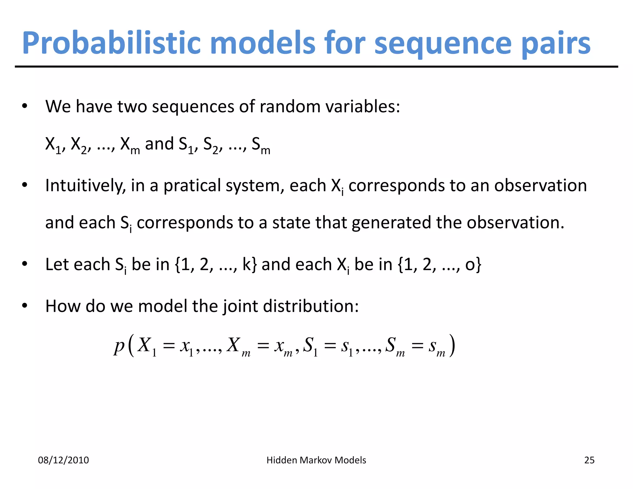
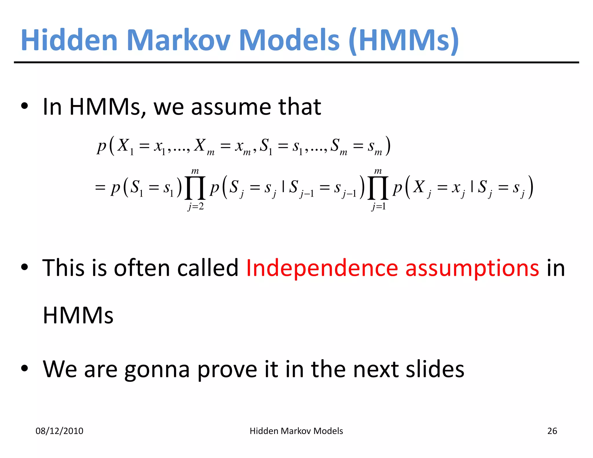
p ( X 1 = x1 ,..., X m = xm , S1 = s1 ,..., S m = sm )
= p ( S1 = s1 ,..., S m = sm ) ×
p ( X 1 = x1 ,..., X m = xm ˚ S1 = s1 ,..., S m = sm )
• Assumption 1: the state sequence forms a Markov chain
m
p ( S1 = s1 ,..., S m = sm ) = p ( S1 = s1 ) ∏ p ( S j = s j ˚ S j −1 = s j −1 )
j =2
08/12/2010 Hidden Markov Models 27](https://image.slidesharecdn.com/hmm-101205115241-phpapp01/75/Hidden-Markov-Models-27-2048.jpg)
![Independence Assumptions in HMMs [2]
• By the chain rule, the following equality is exact:
p ( X 1 = x1 ,..., X m = xm ˚ S1 = s1 ,..., S m = sm )
m
= ∏ p ( X j = x j ˚ S1 = s1 ,..., Sm = sm , X 1 = x1 ,..., X j −1 = x j −1 )
j =1
• Assumption 2: each observation depends only on the underlying
state
p ( X j = x j ˚ S1 = s1 ,..., Sm = sm , X 1 = x1 ,..., X j −1 = x j −1 )
= p( X j = xj ˚ S j = sj )
• These two assumptions are often called independence
assumptions in HMMs
08/12/2010 Hidden Markov Models 28](https://image.slidesharecdn.com/hmm-101205115241-phpapp01/75/Hidden-Markov-Models-28-2048.jpg)


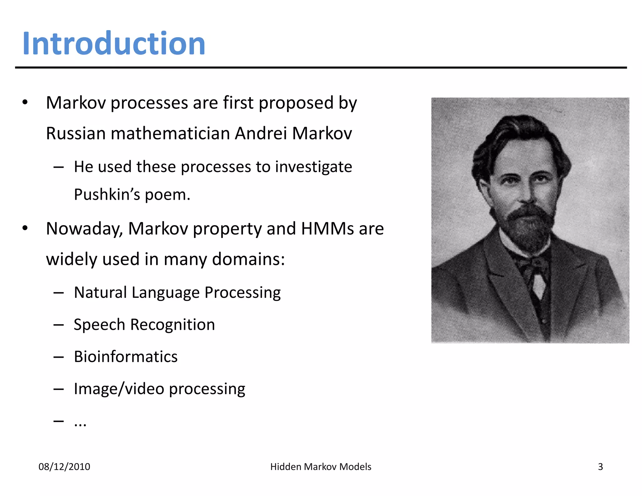
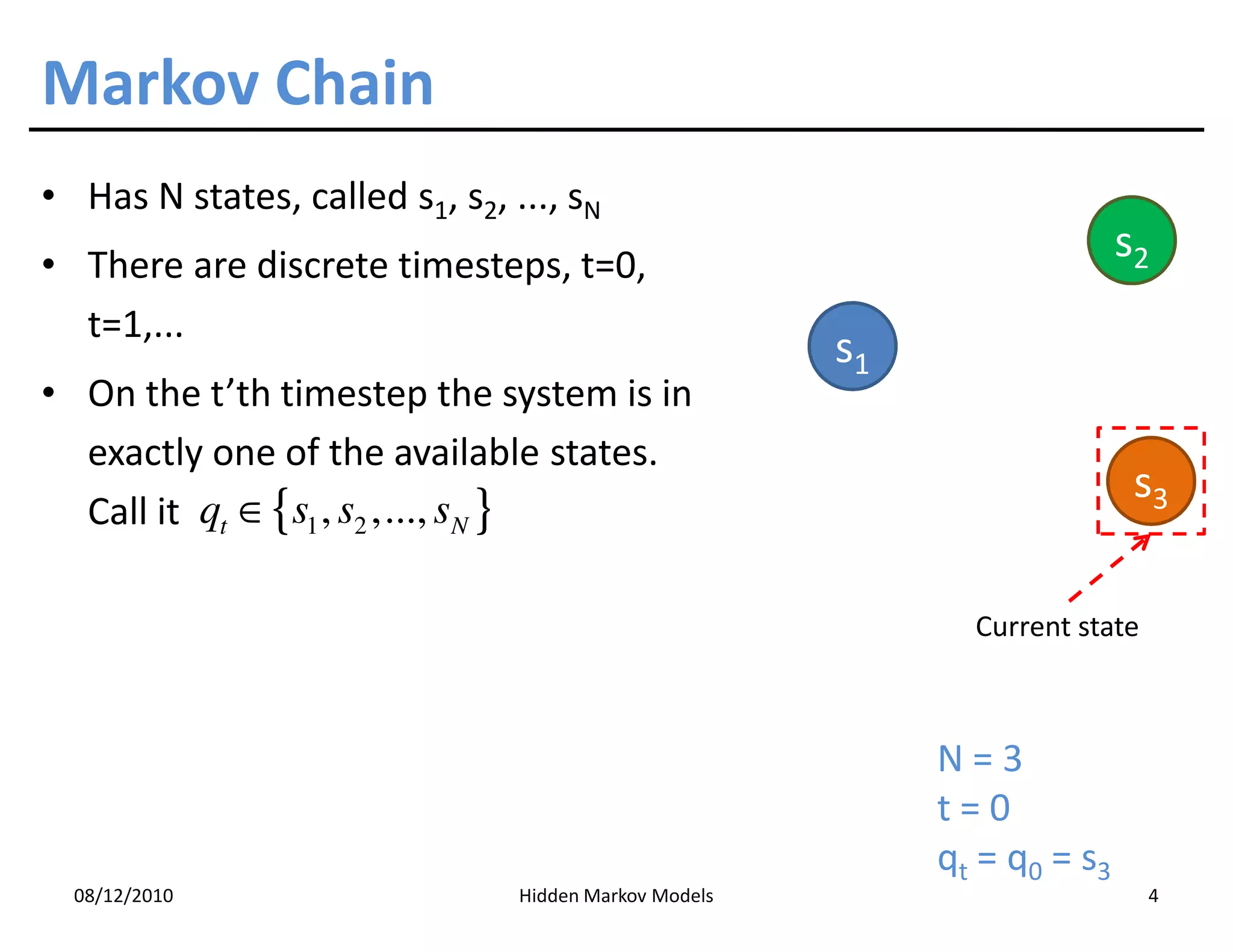
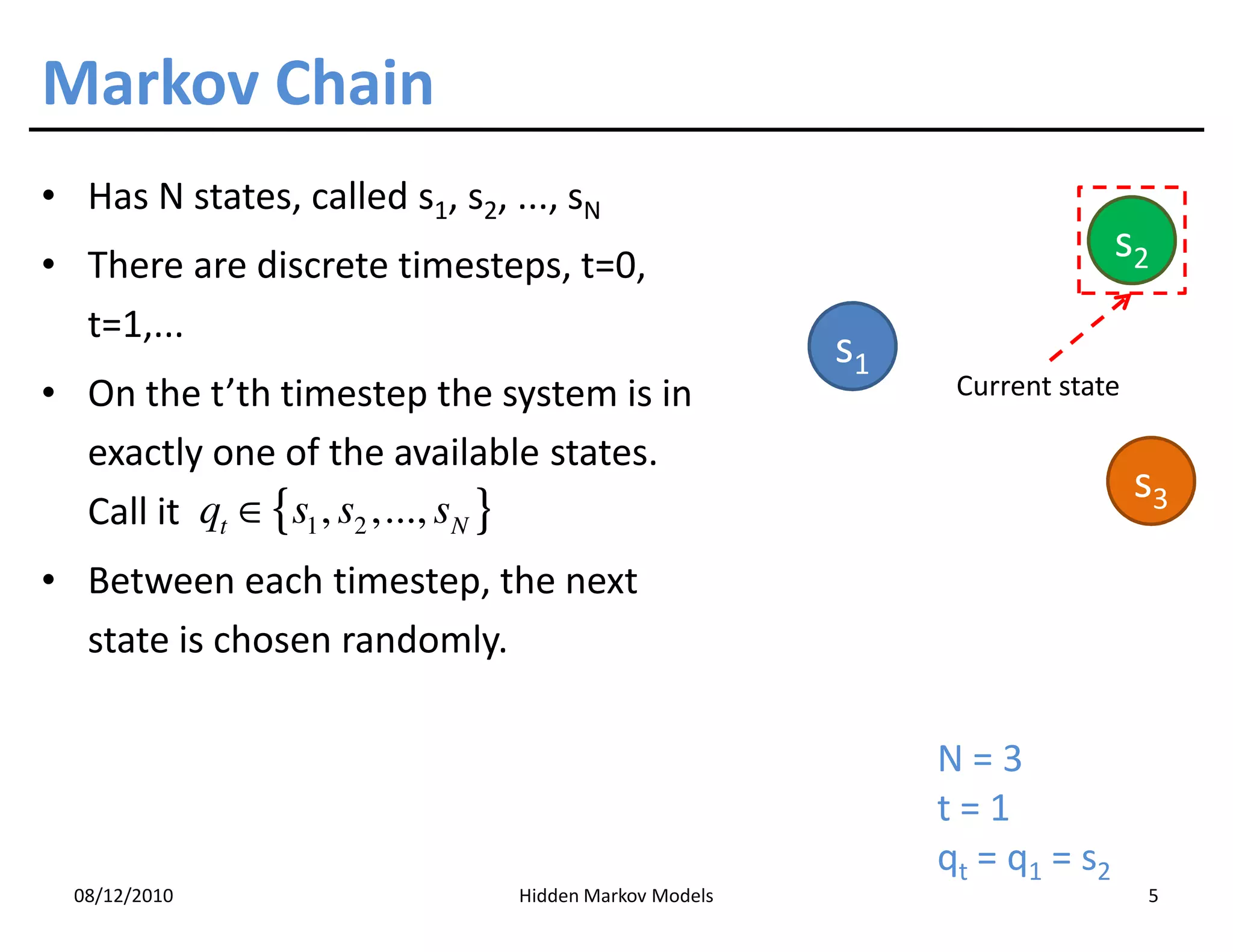
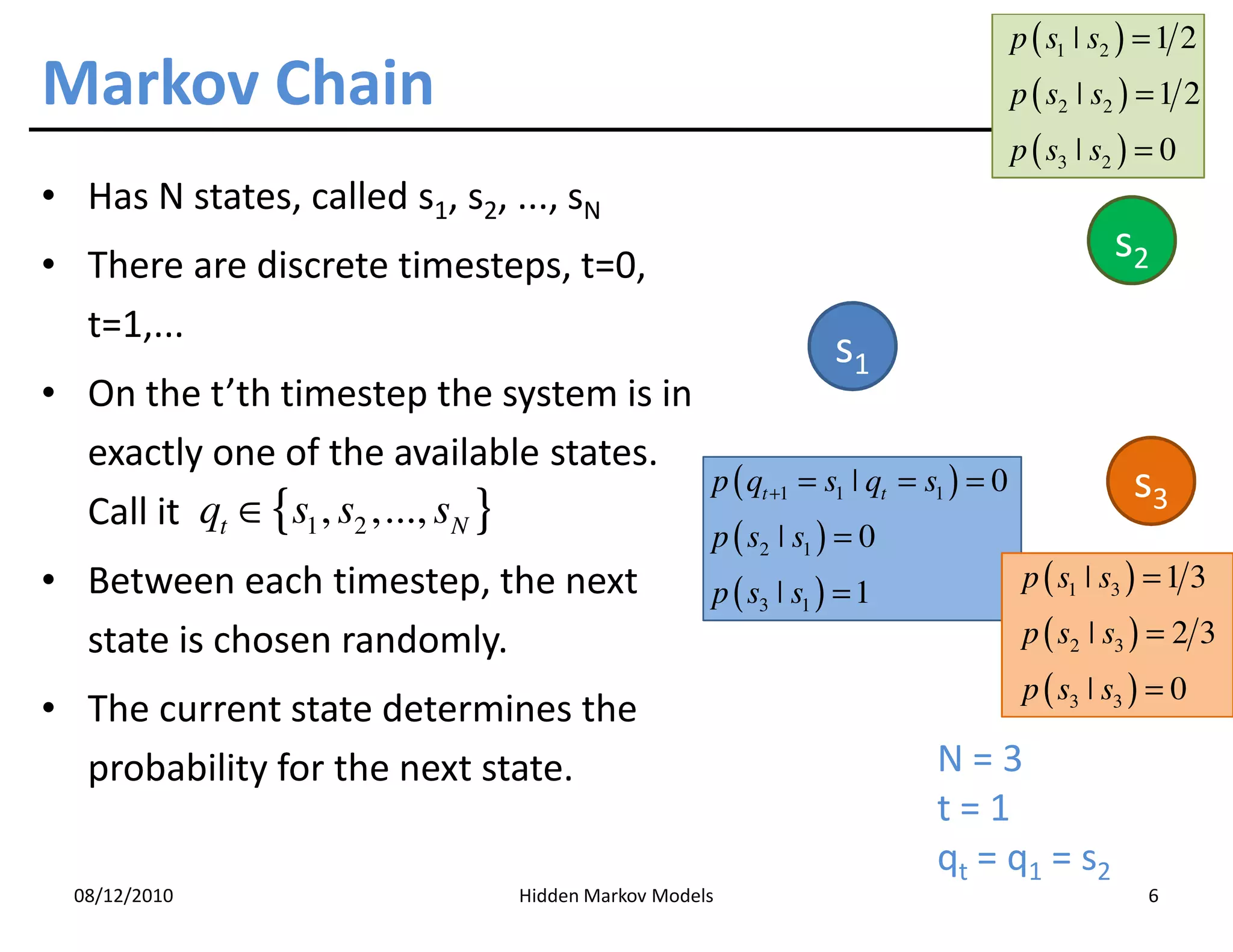
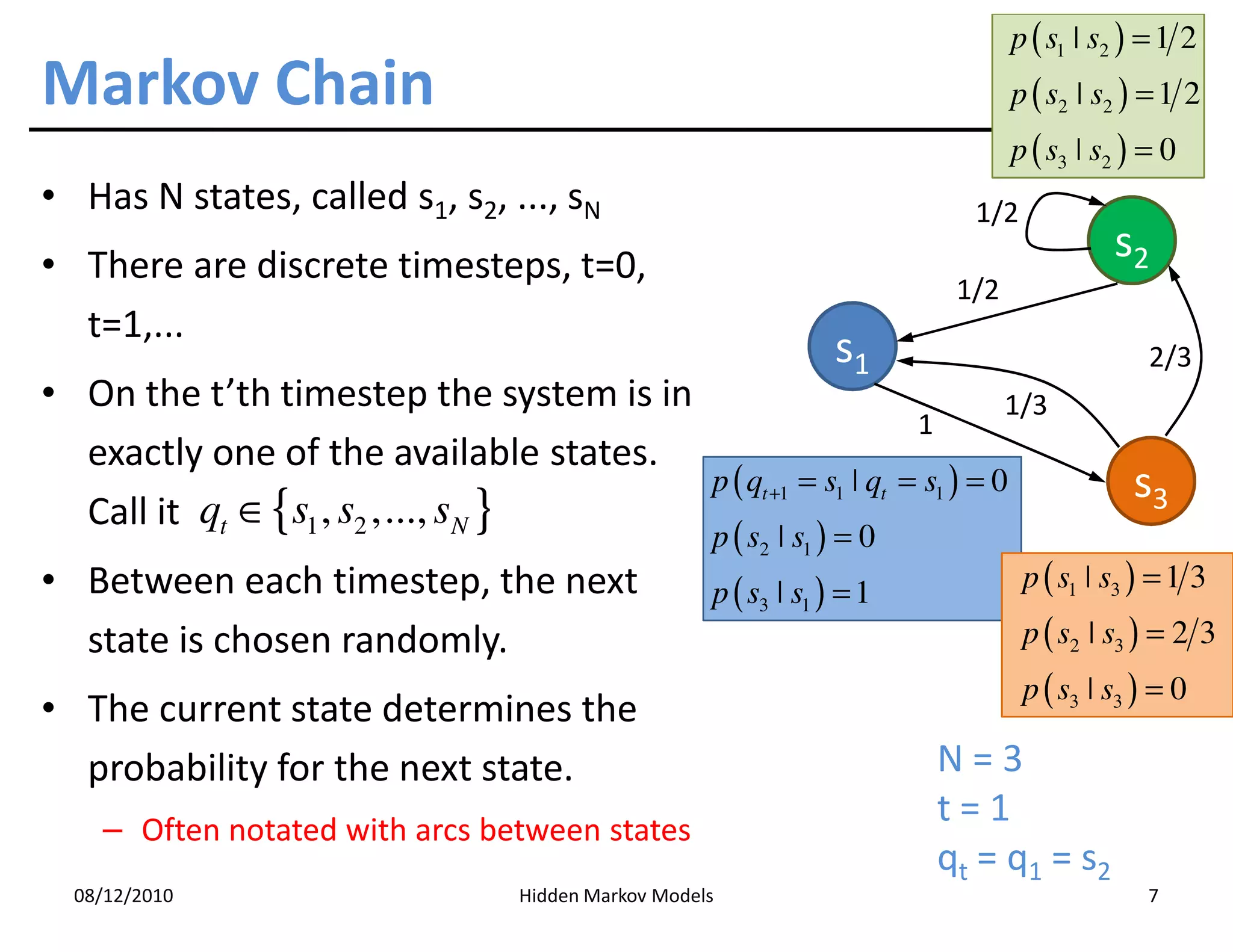
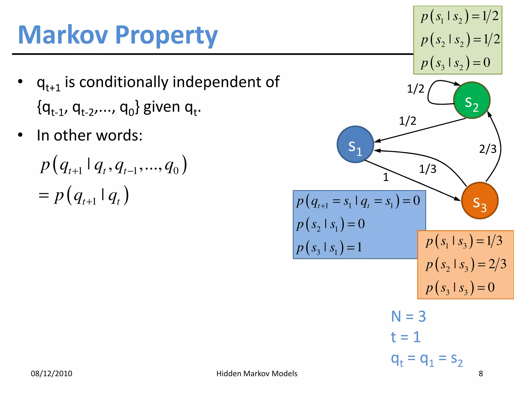
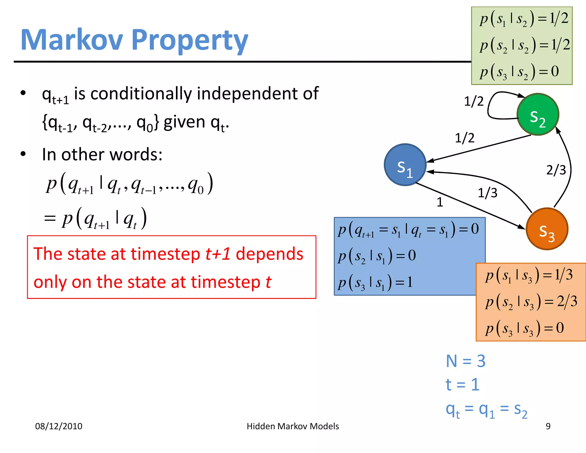
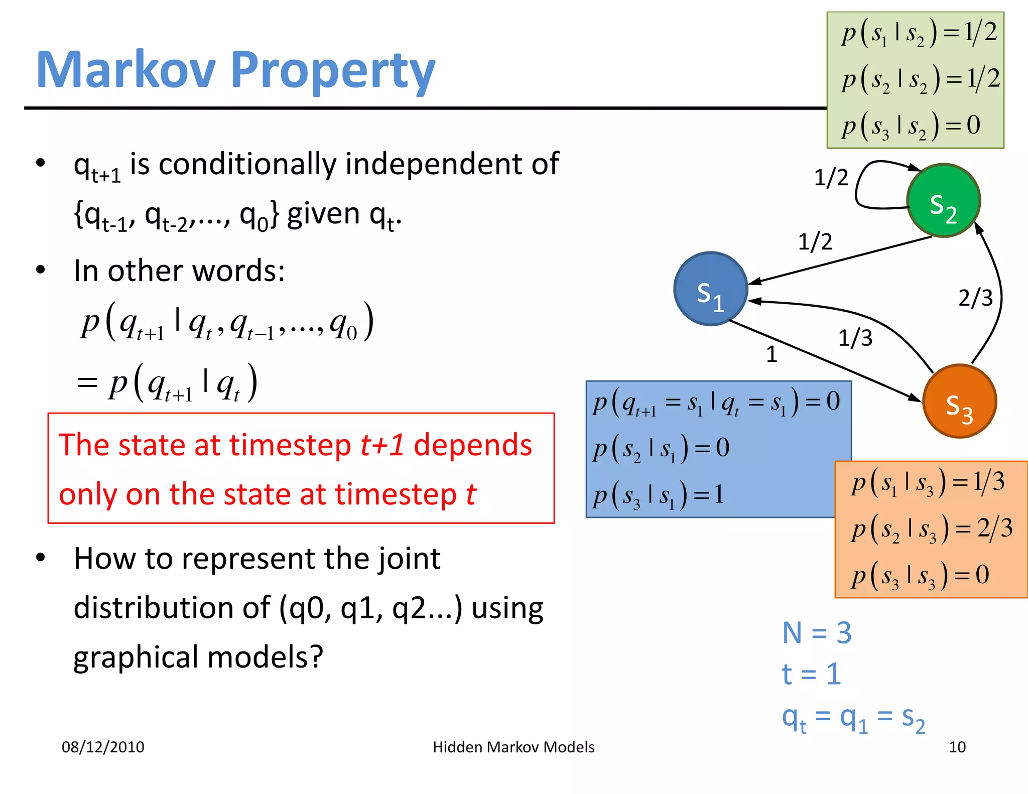
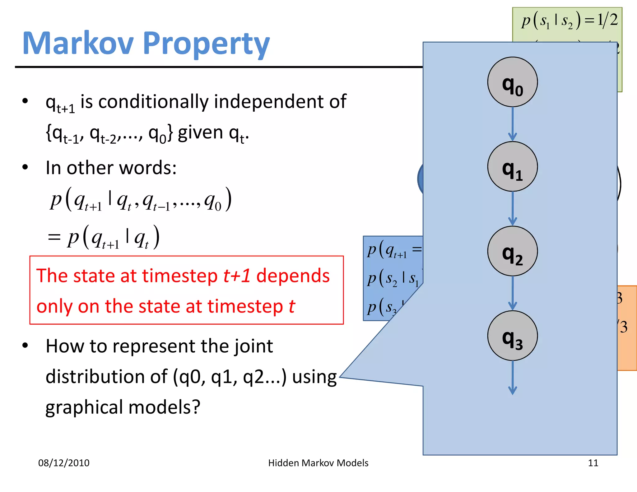
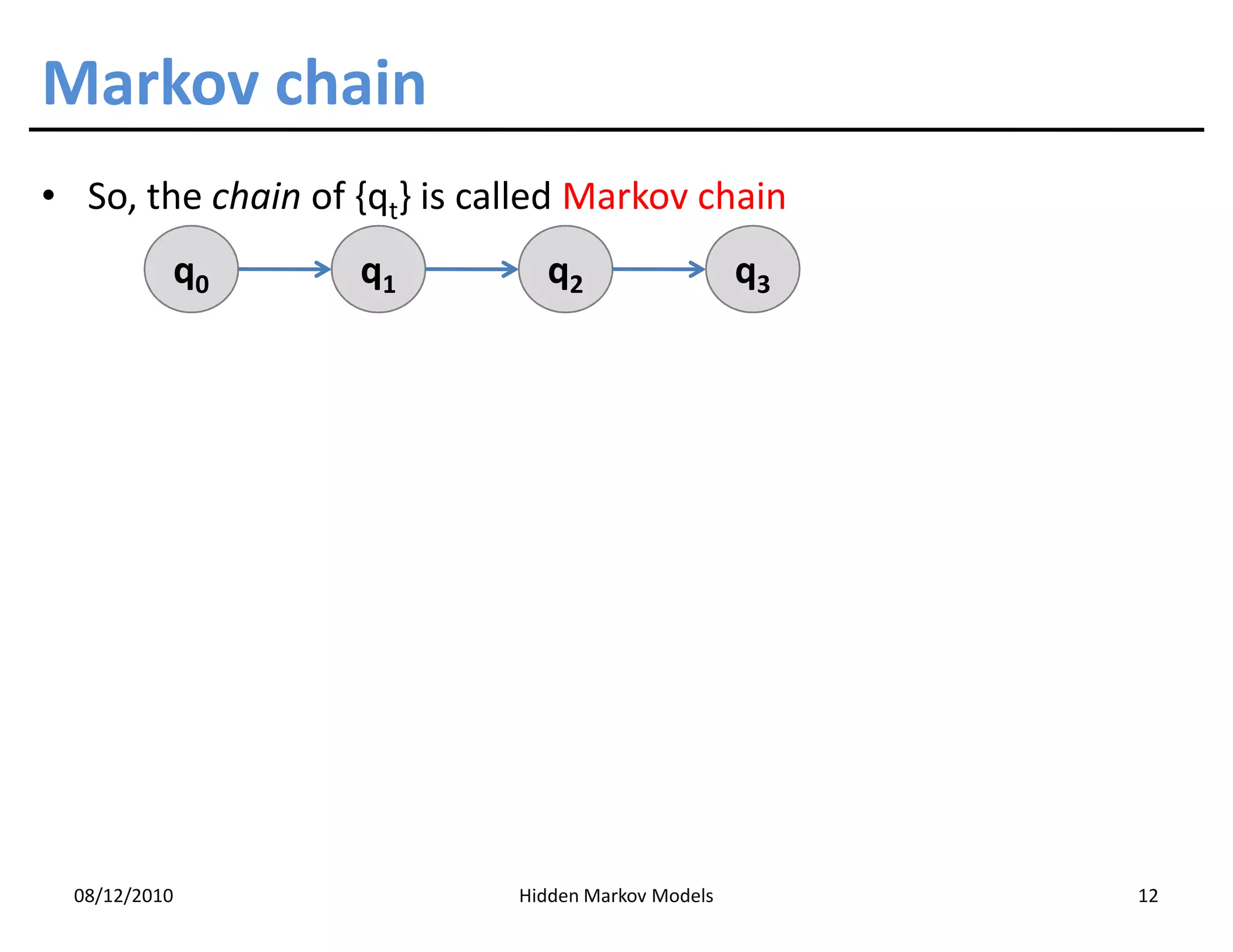
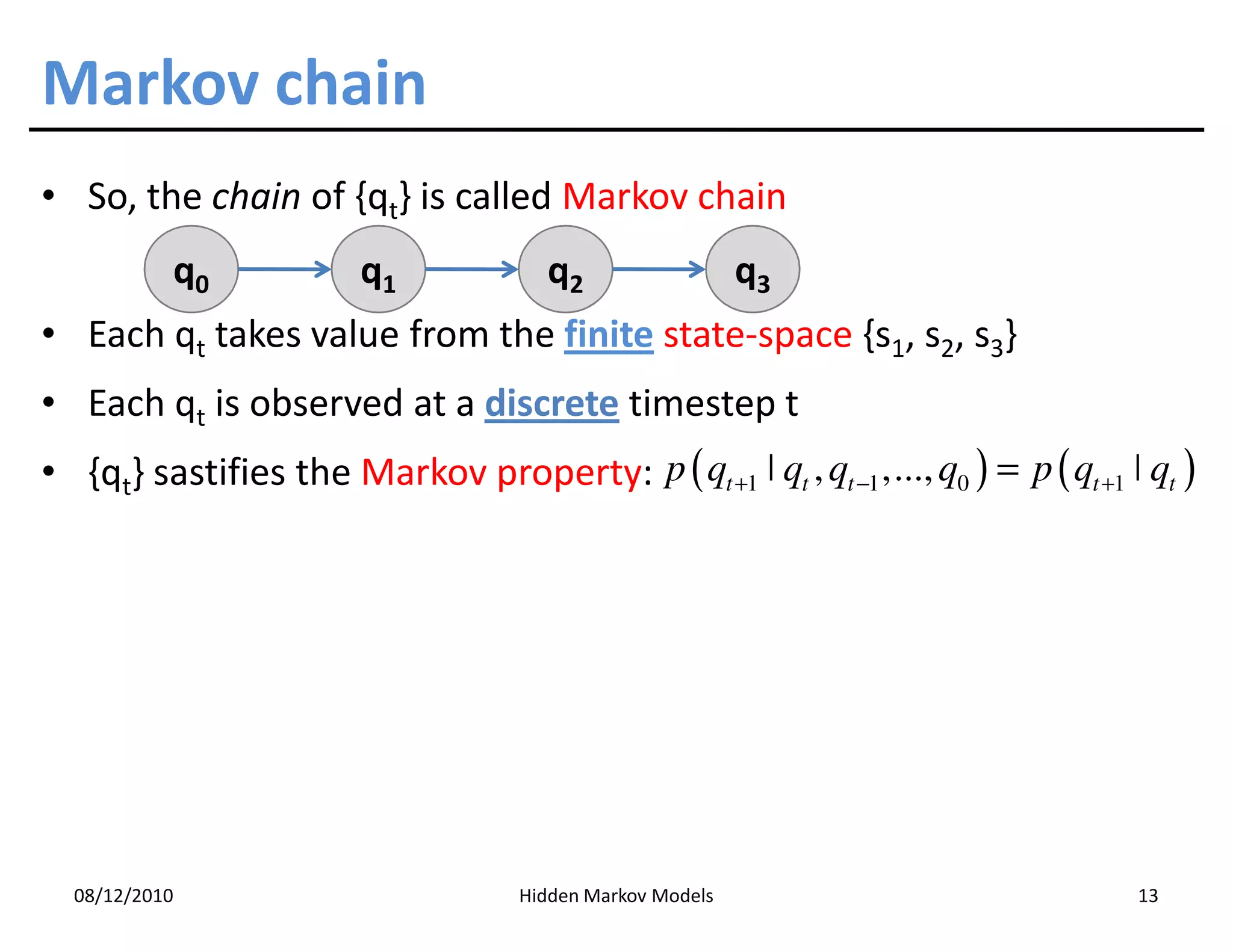
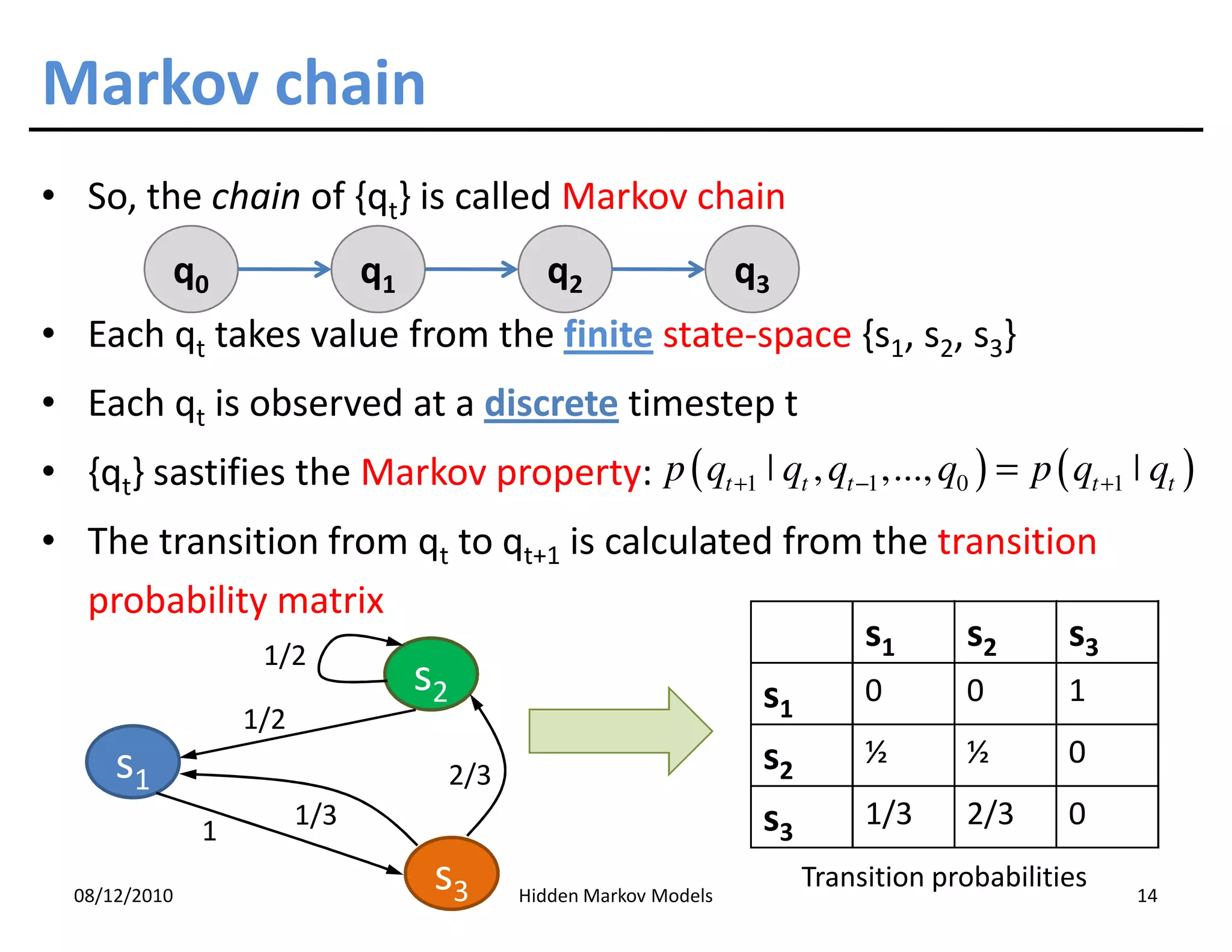
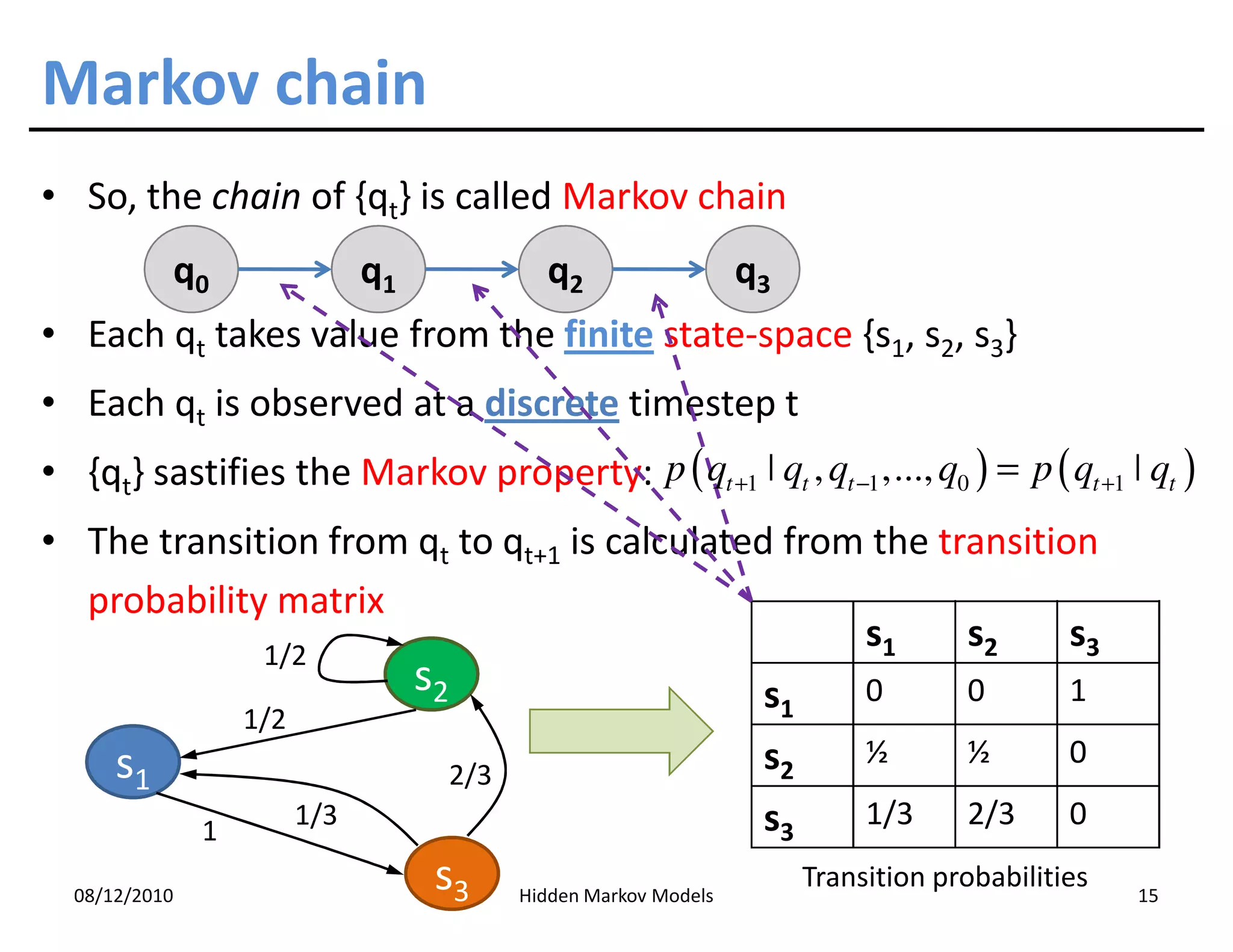
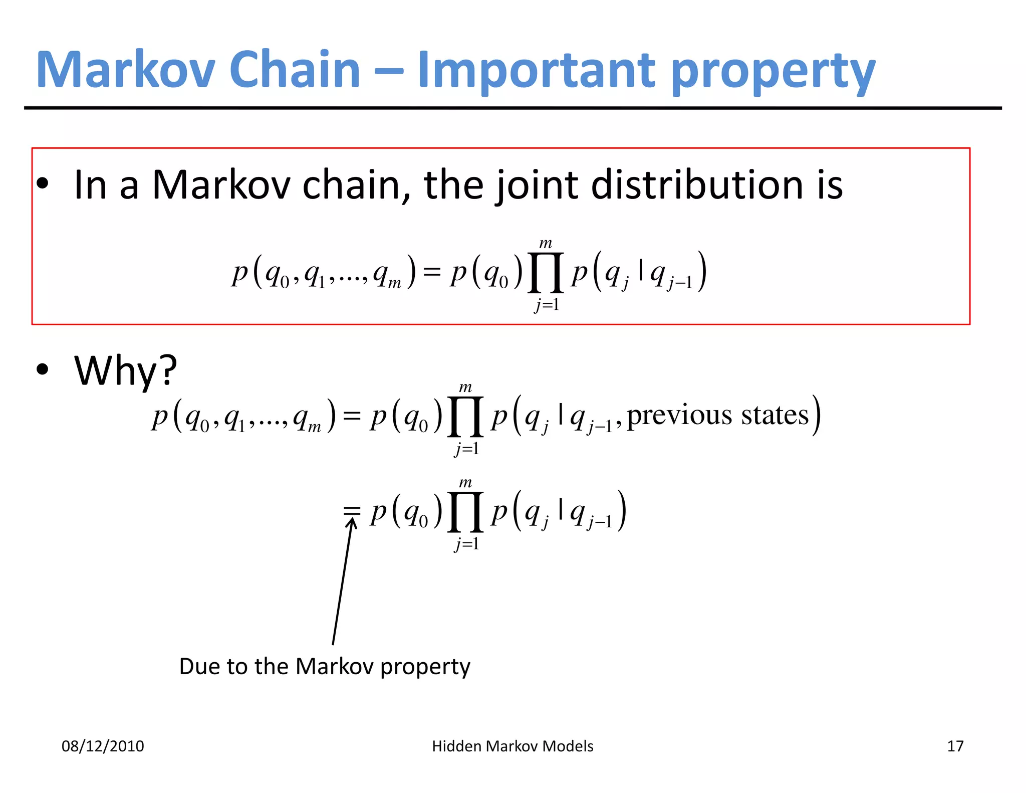
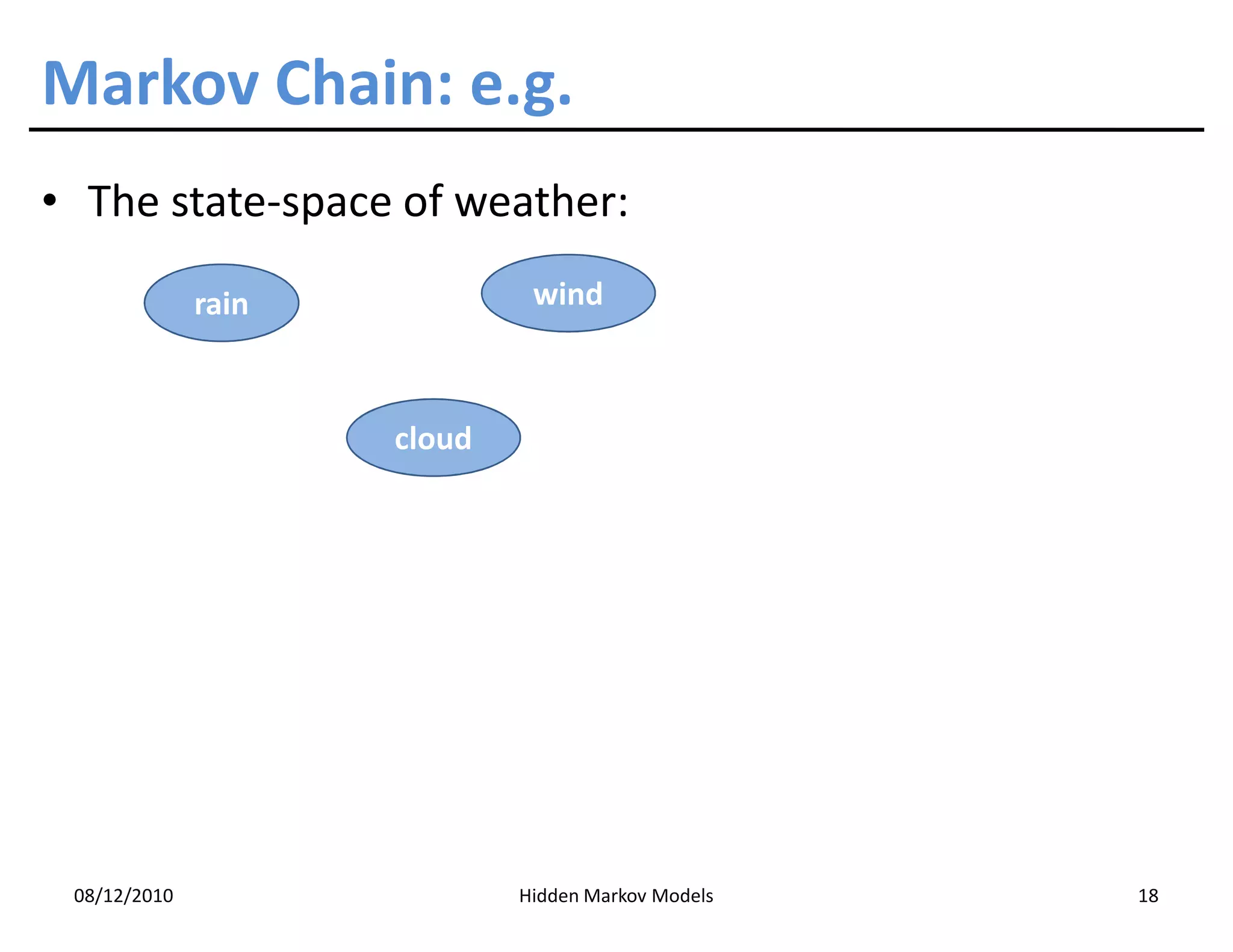
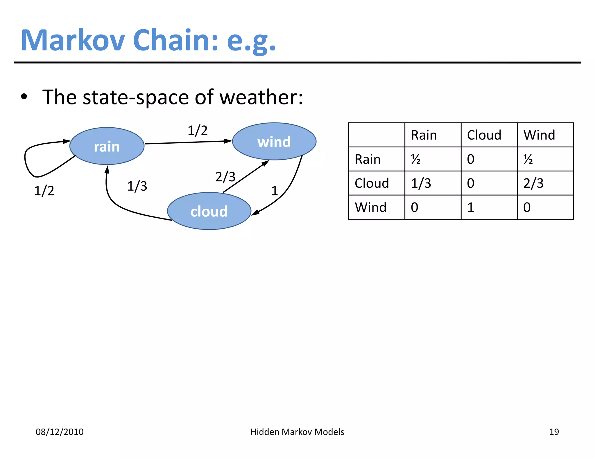
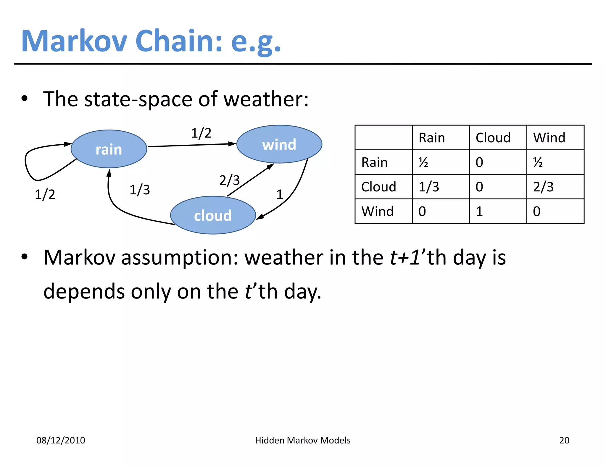
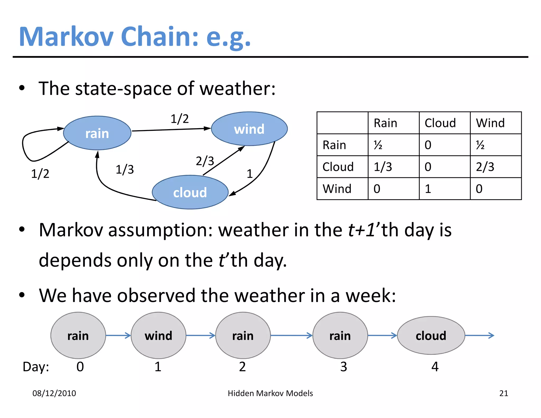
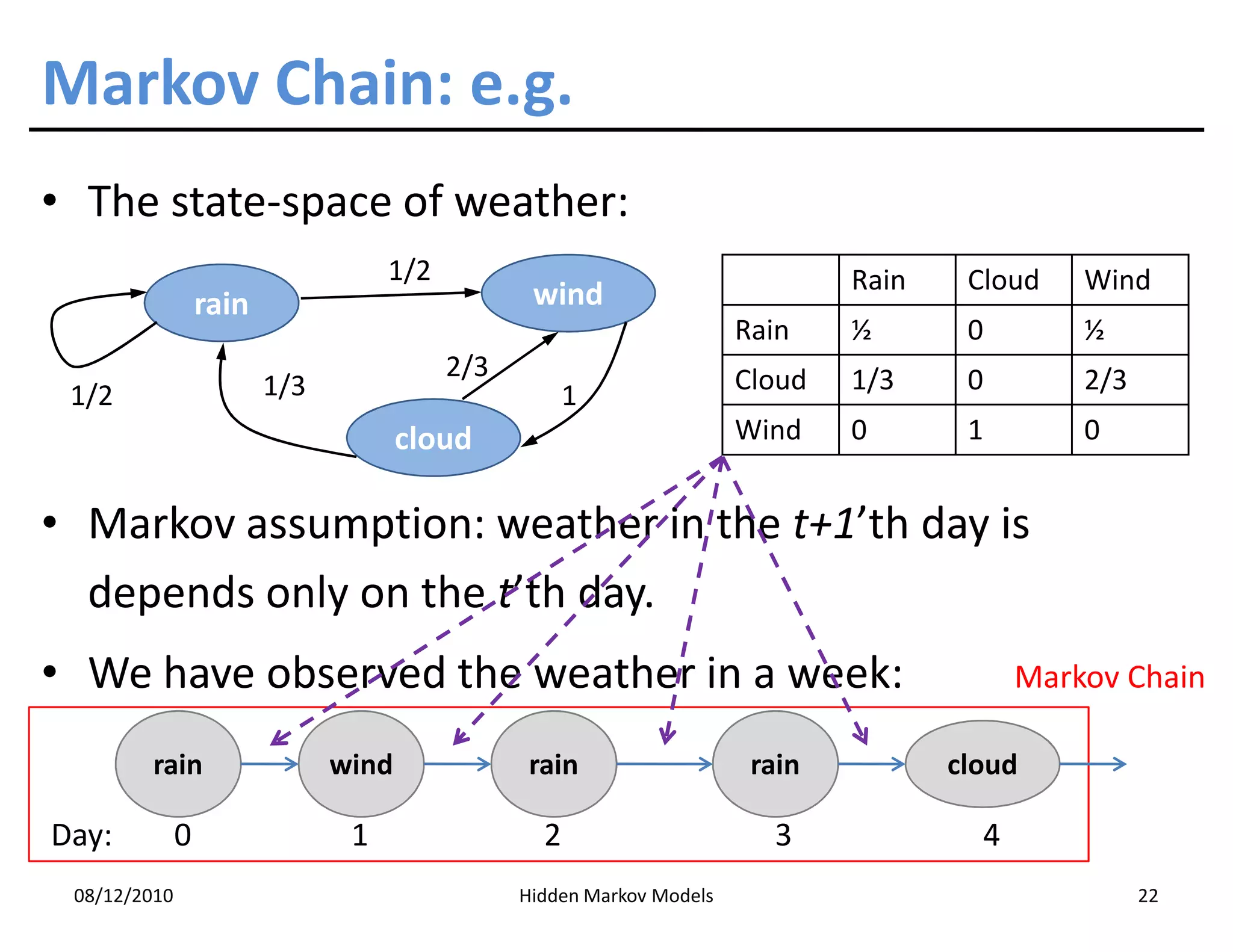
This document discusses Hidden Markov Models (HMMs) and Markov chains. It begins with an introduction to Markov processes and how HMMs are used in various domains like natural language processing. It then describes the properties of a Markov chain, which has a set of states that the system transitions between randomly at discrete time steps based on transition probabilities. The Markov property is explained as the conditional independence of future states from past states given the present state. HMMs extend Markov chains by making the state sequence hidden and only allowing observation of the output states.