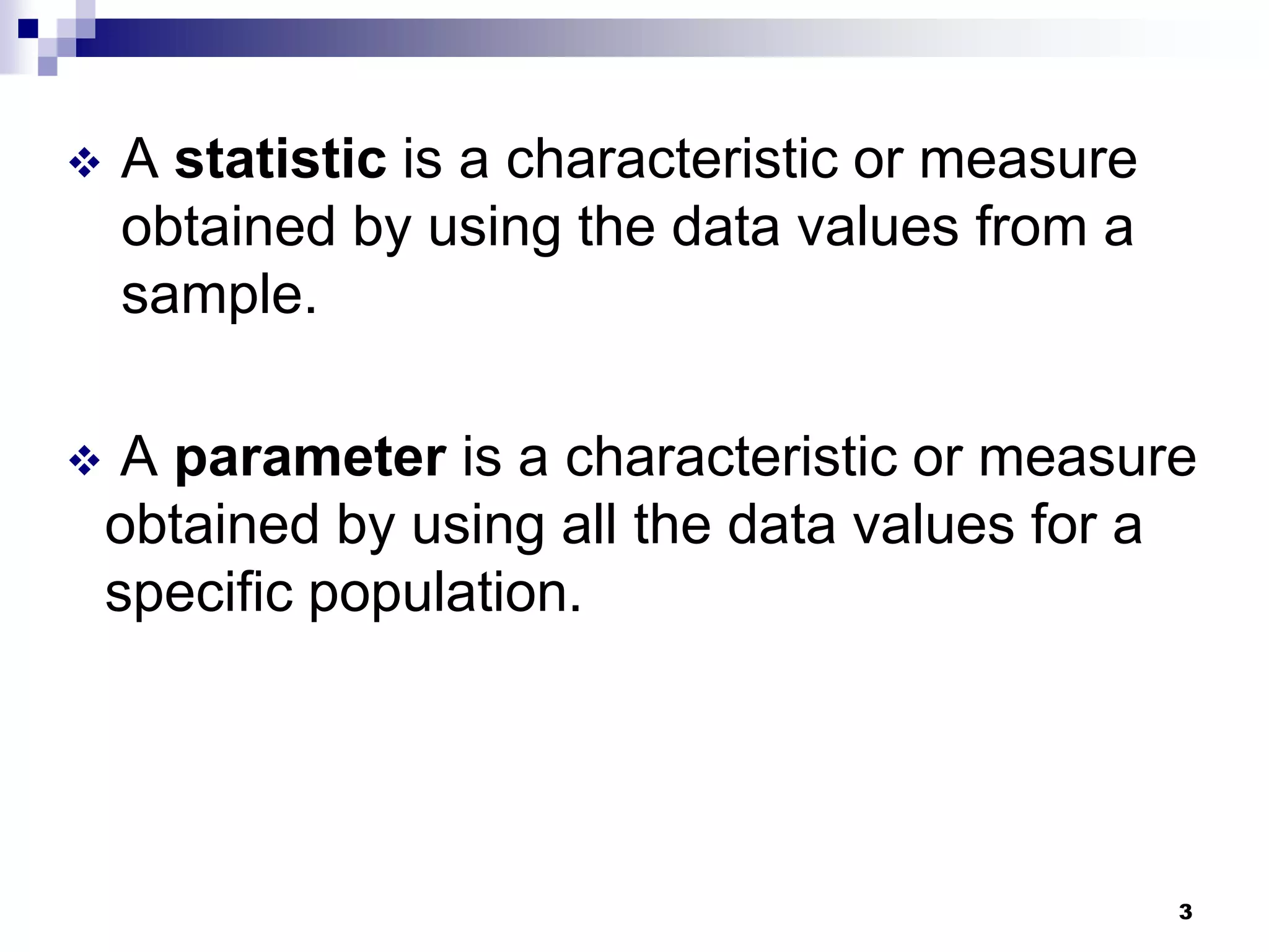
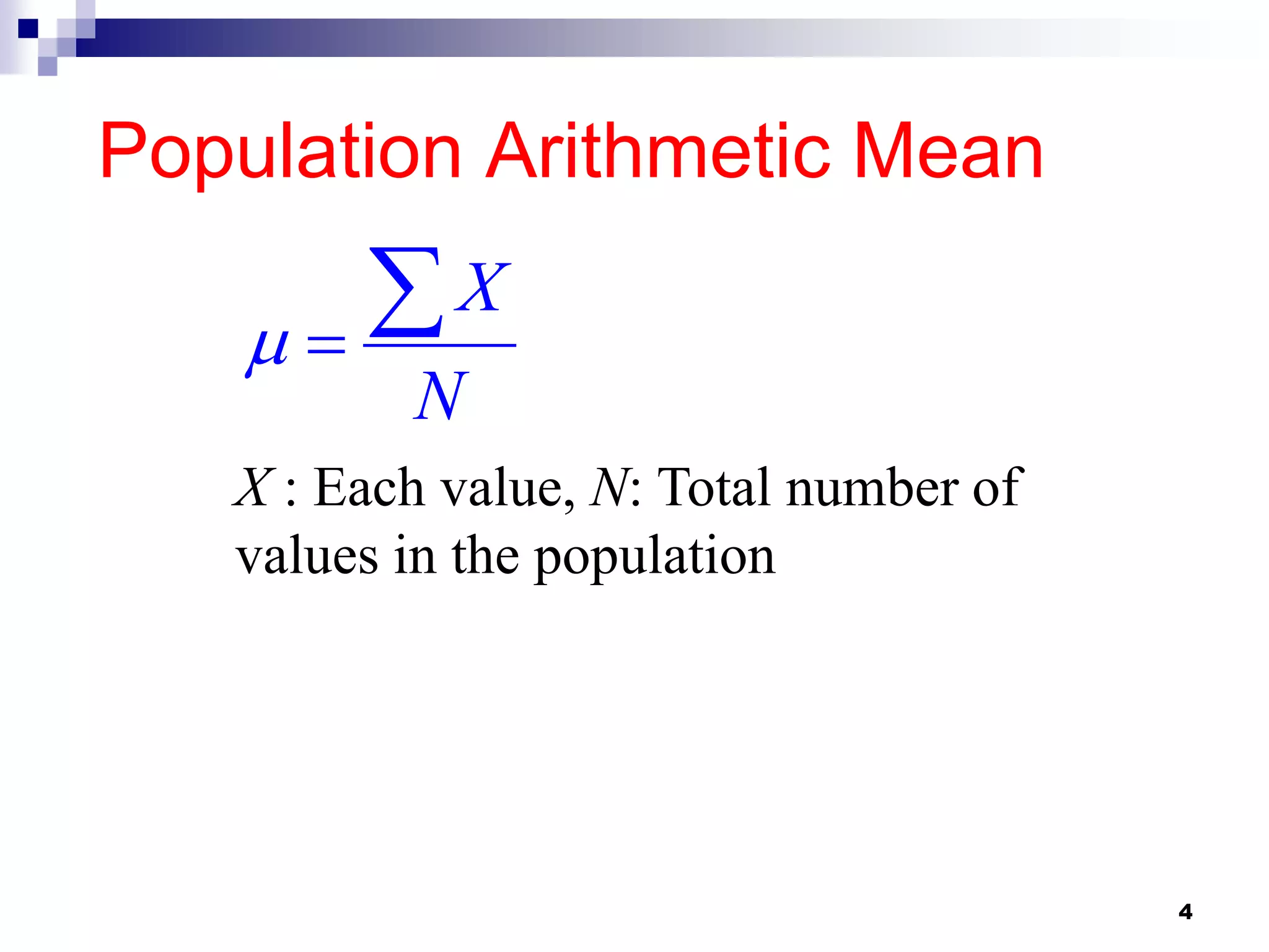
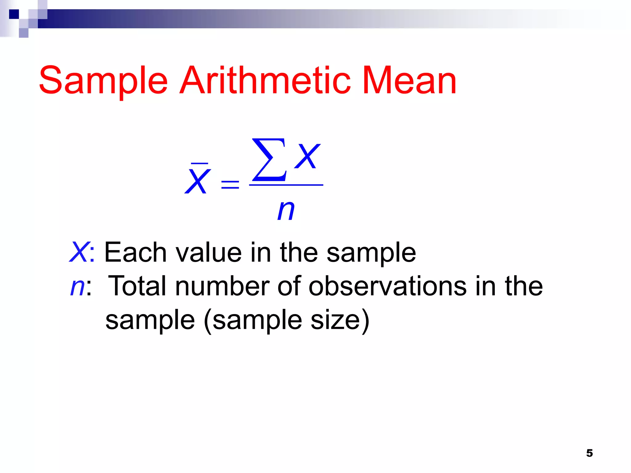
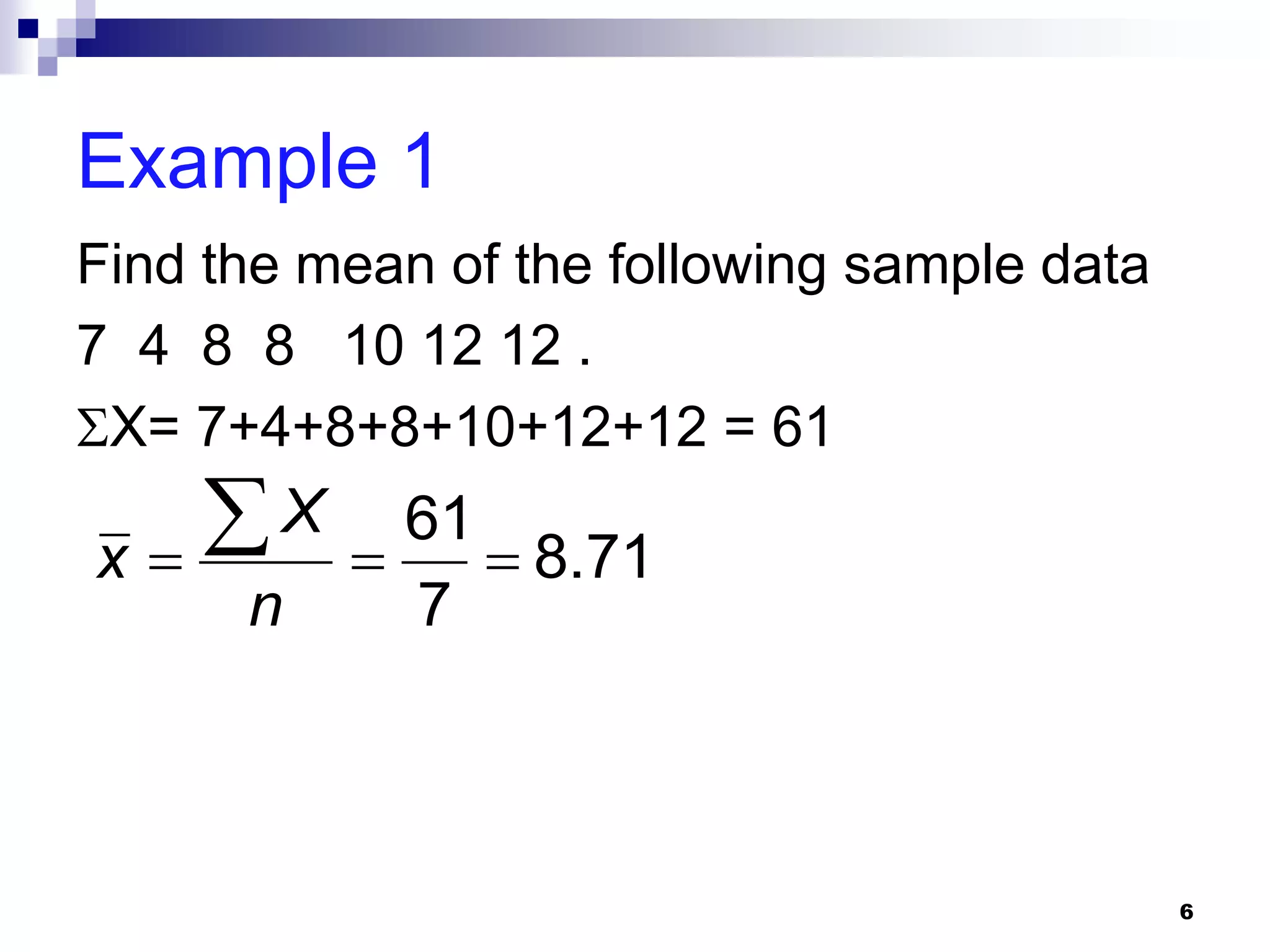
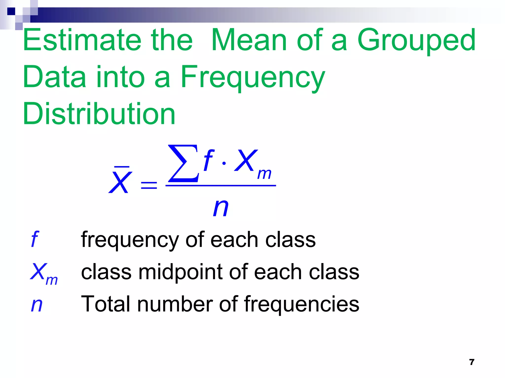
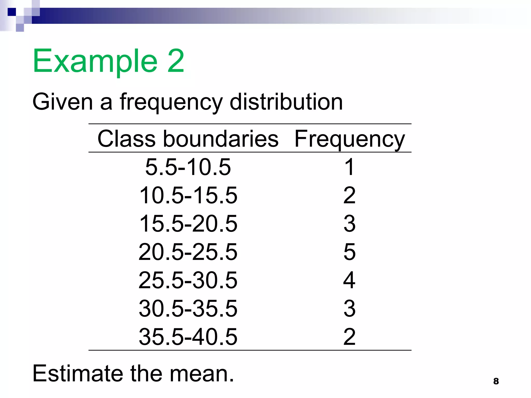
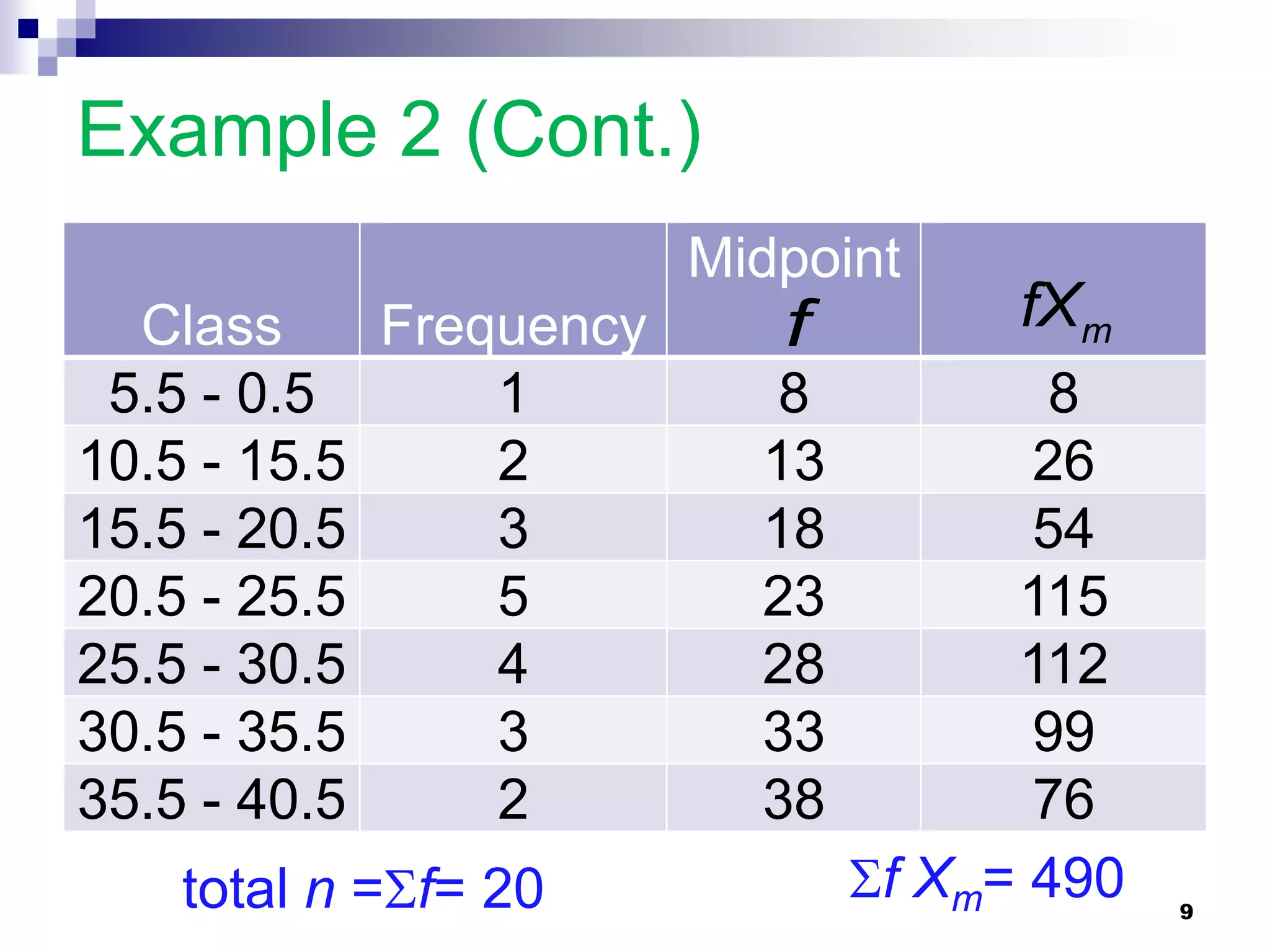
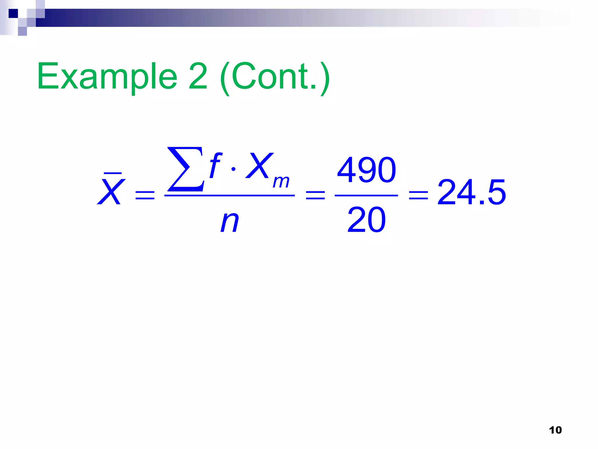
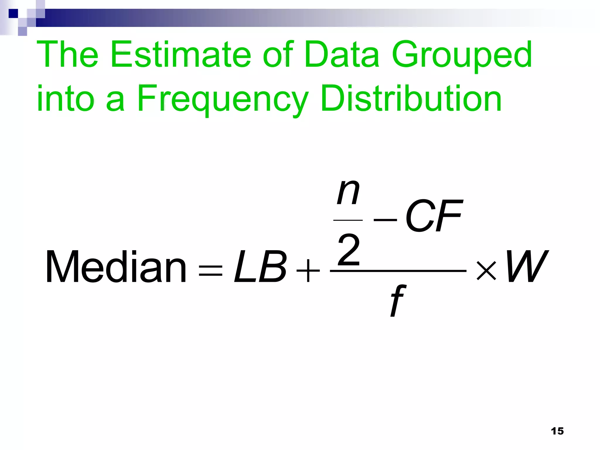
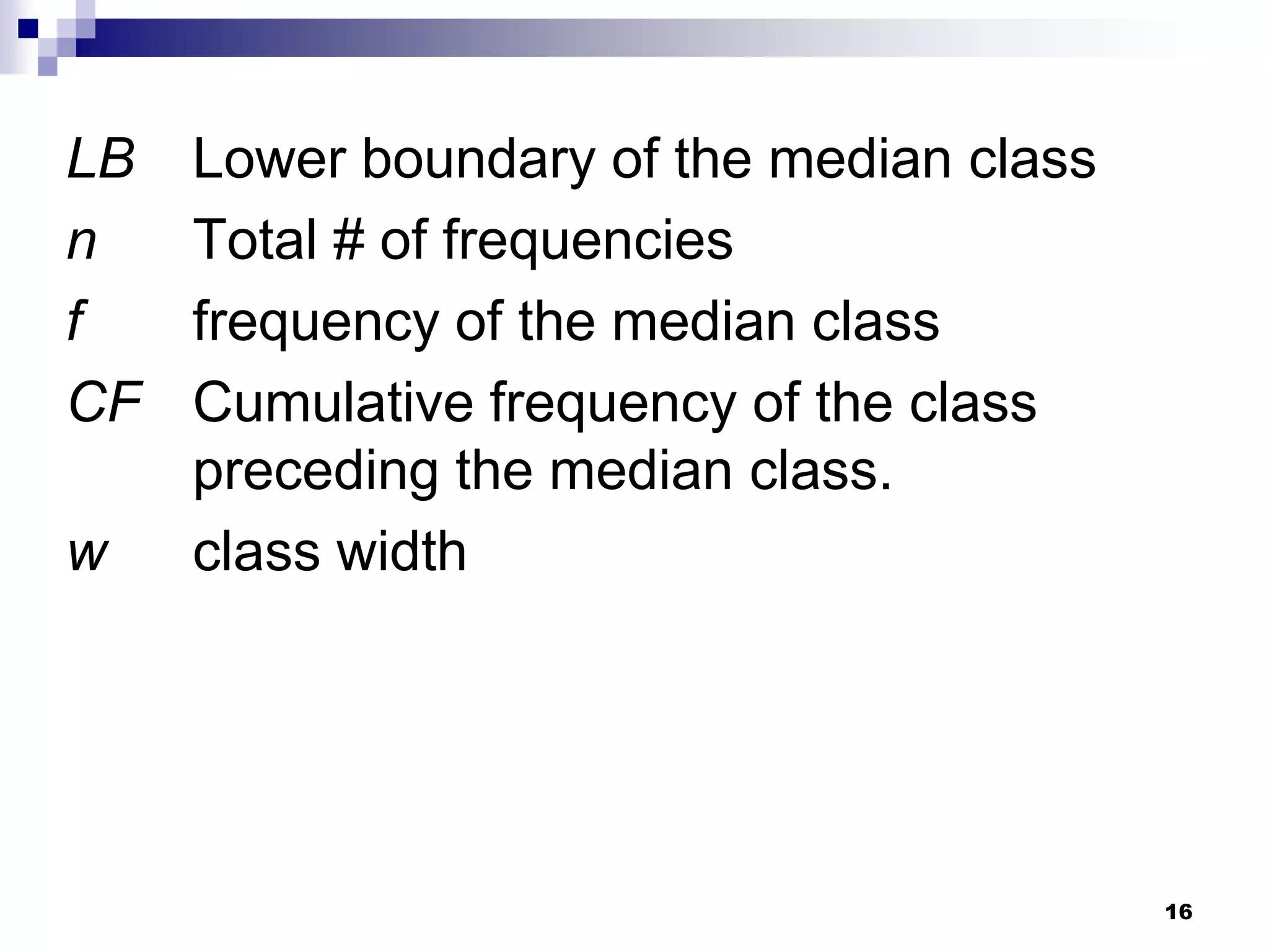
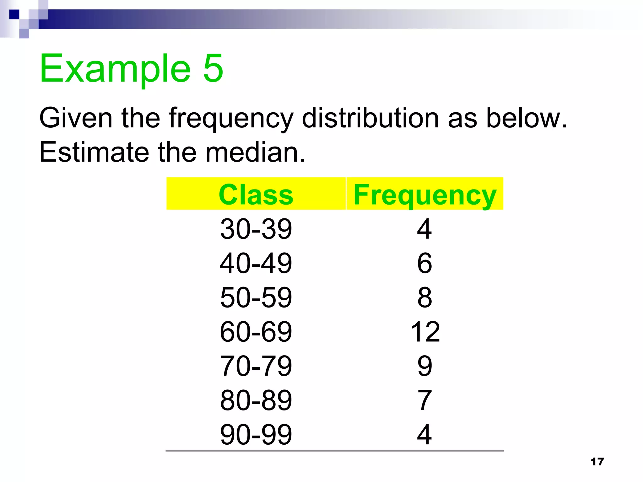
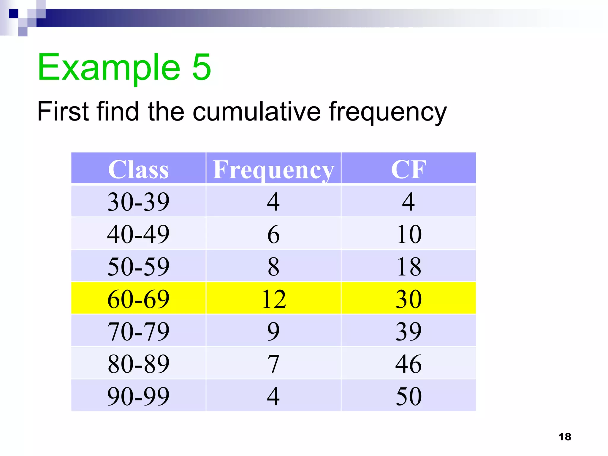
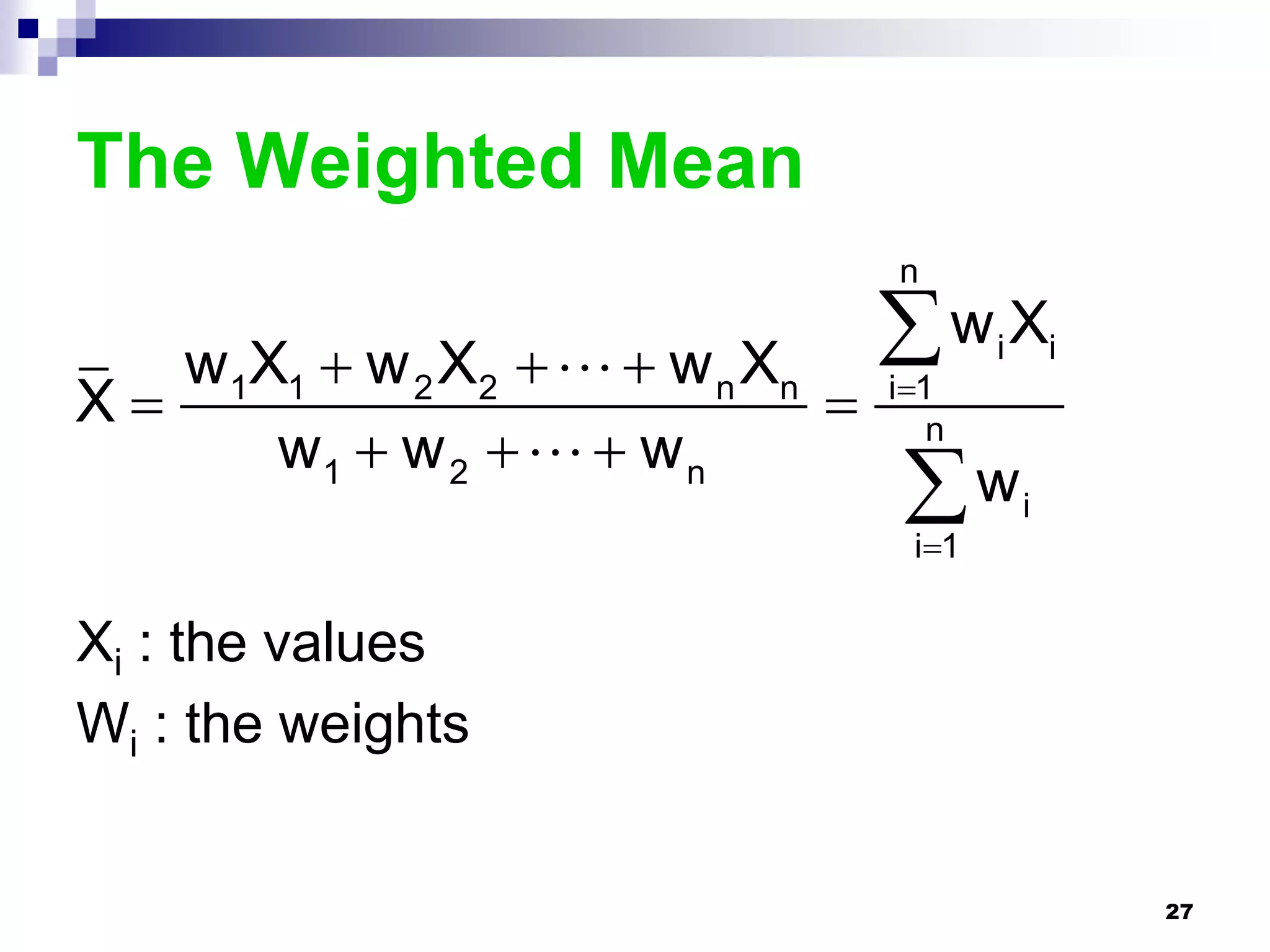
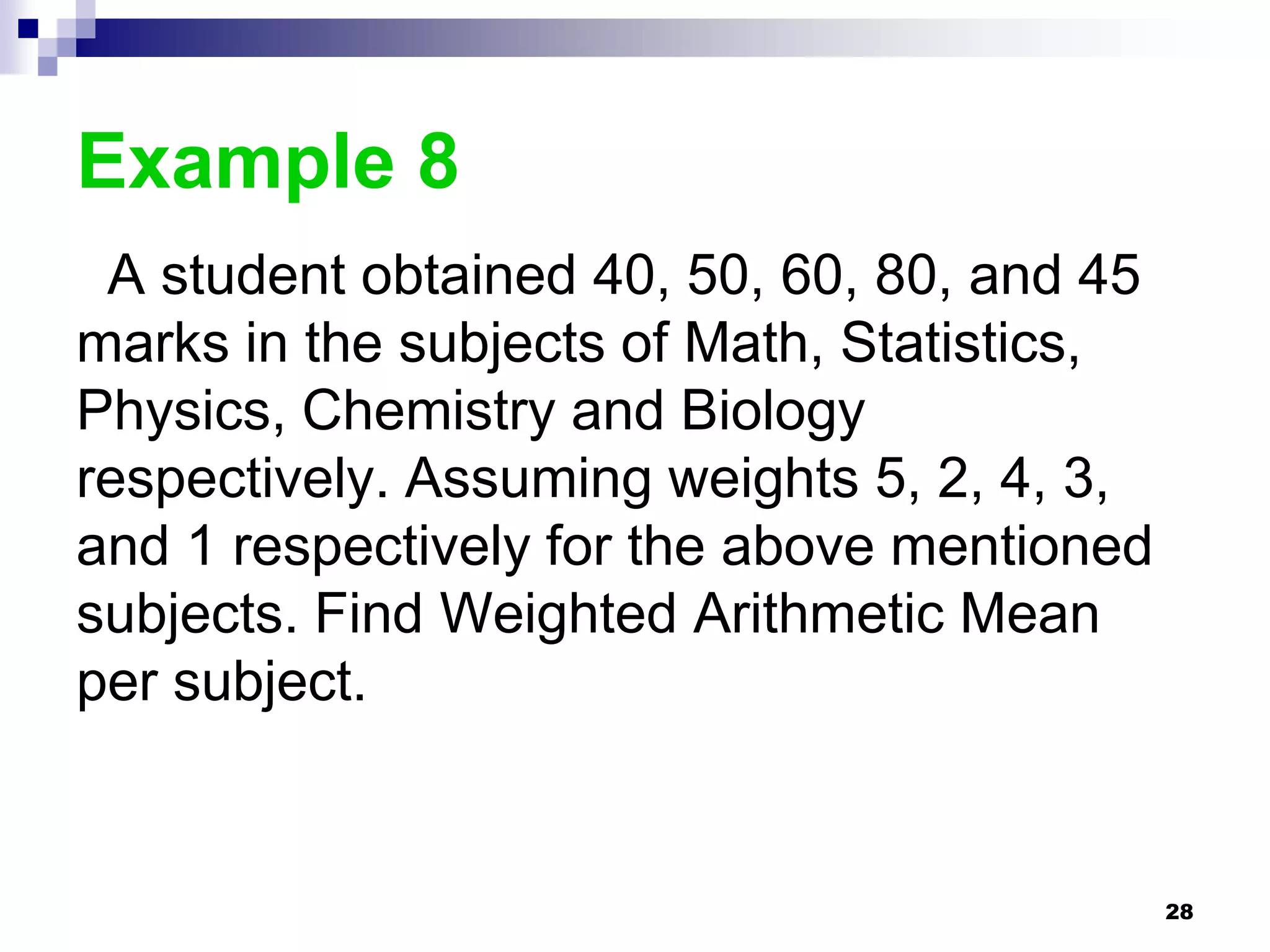
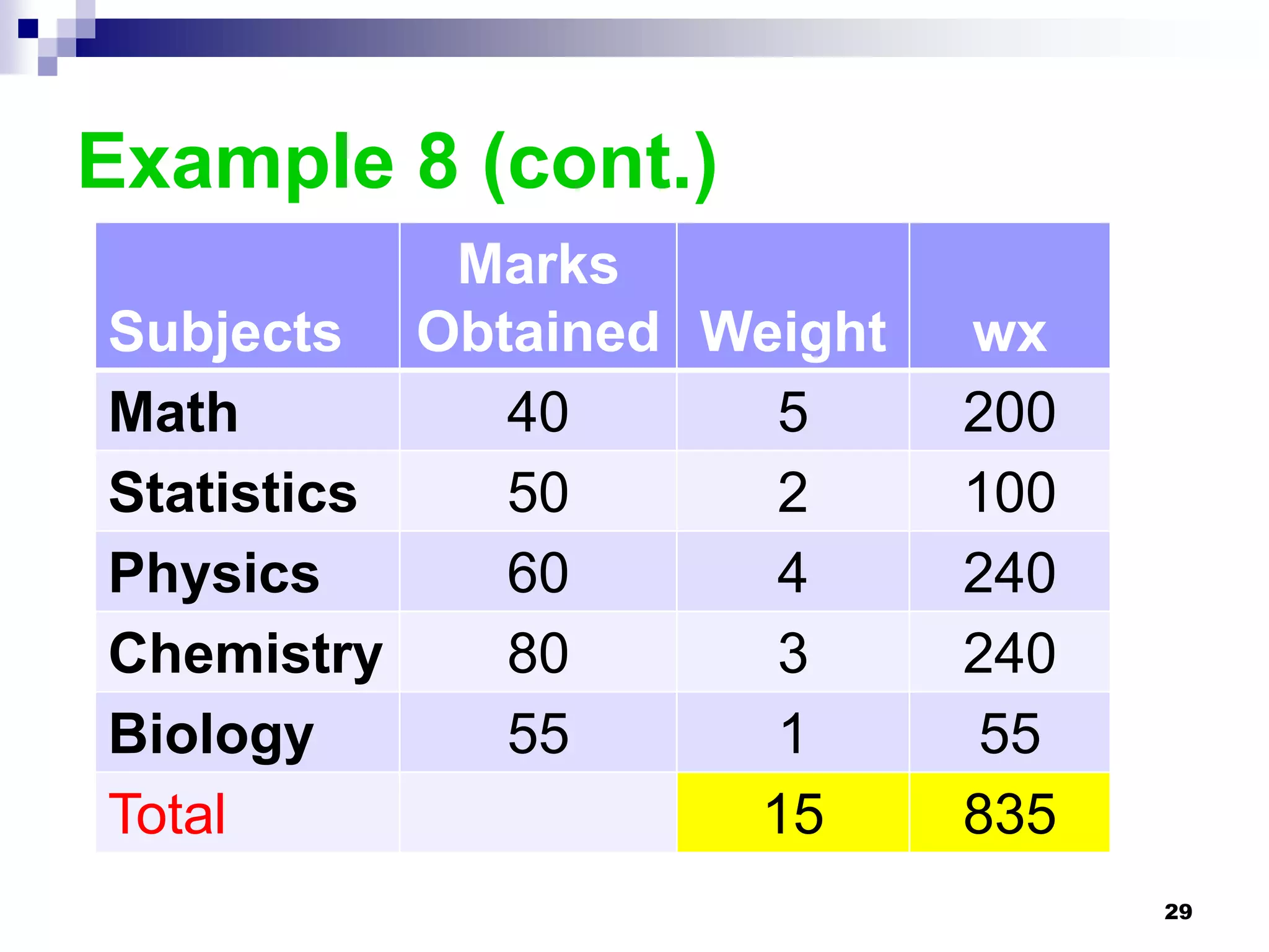
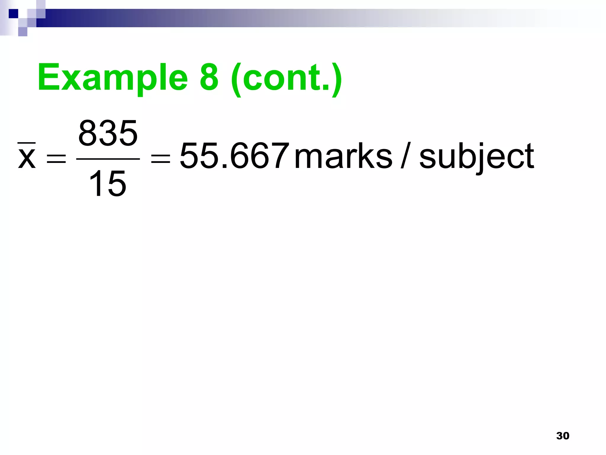
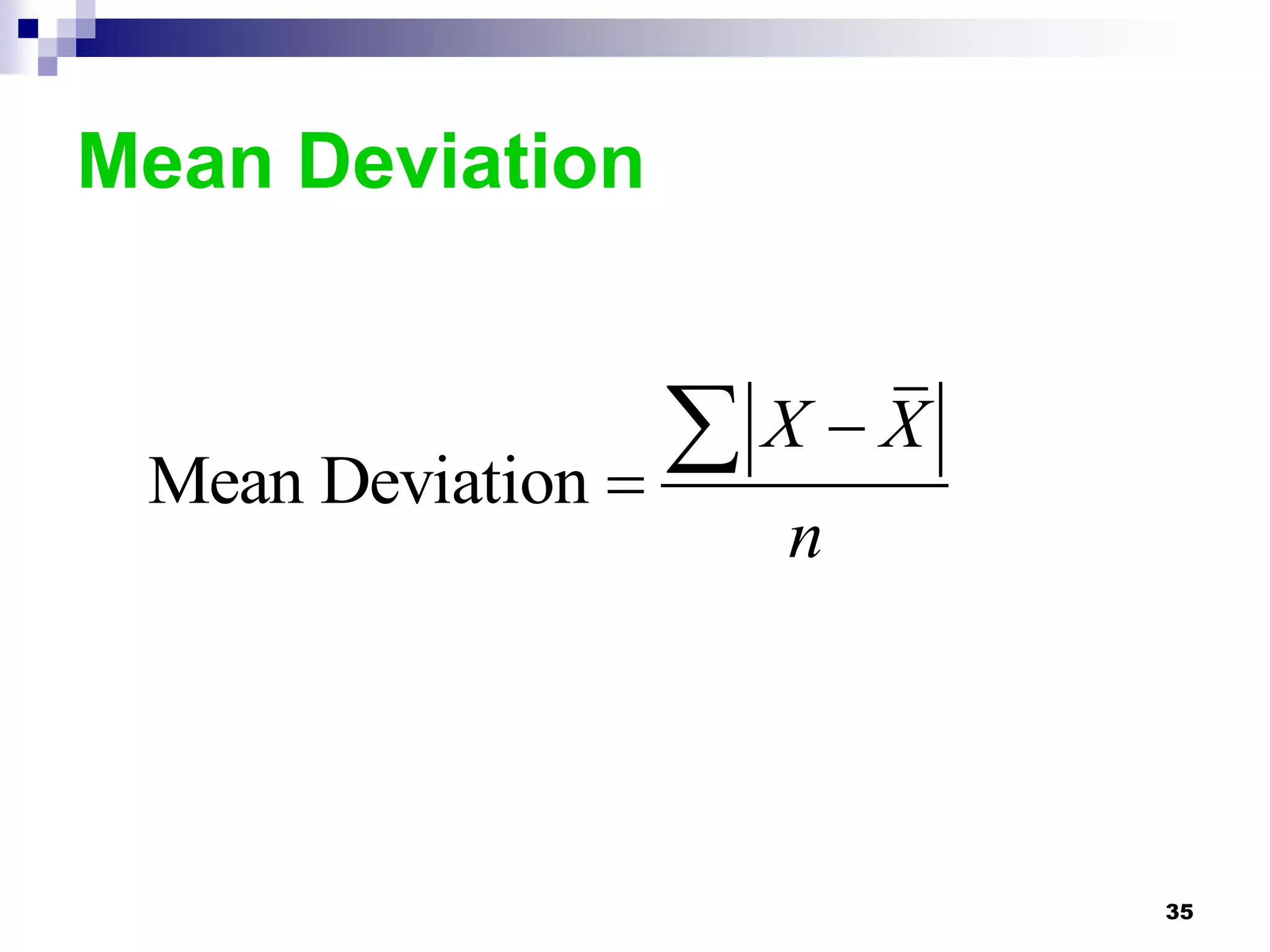
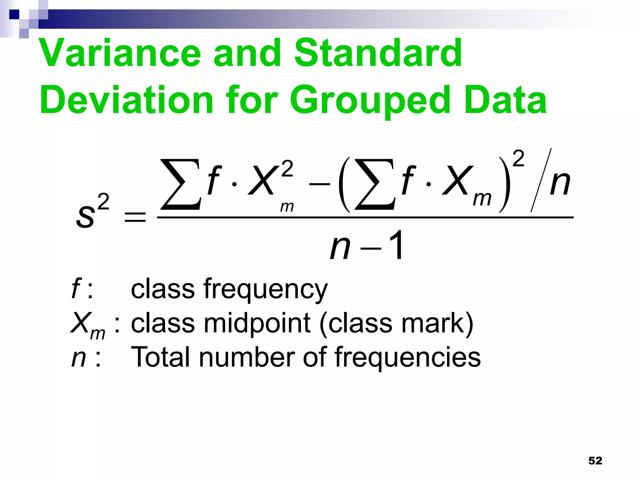
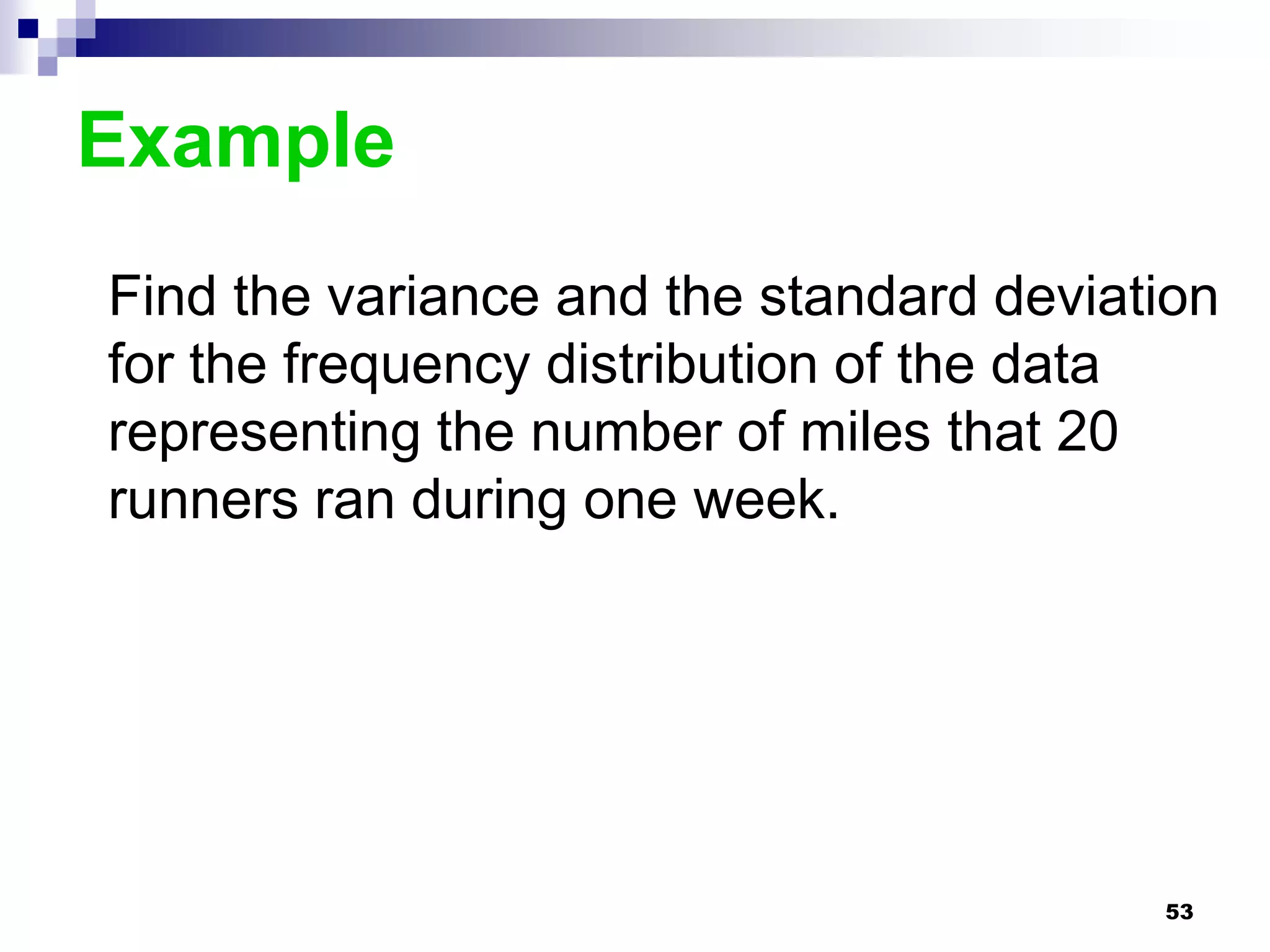
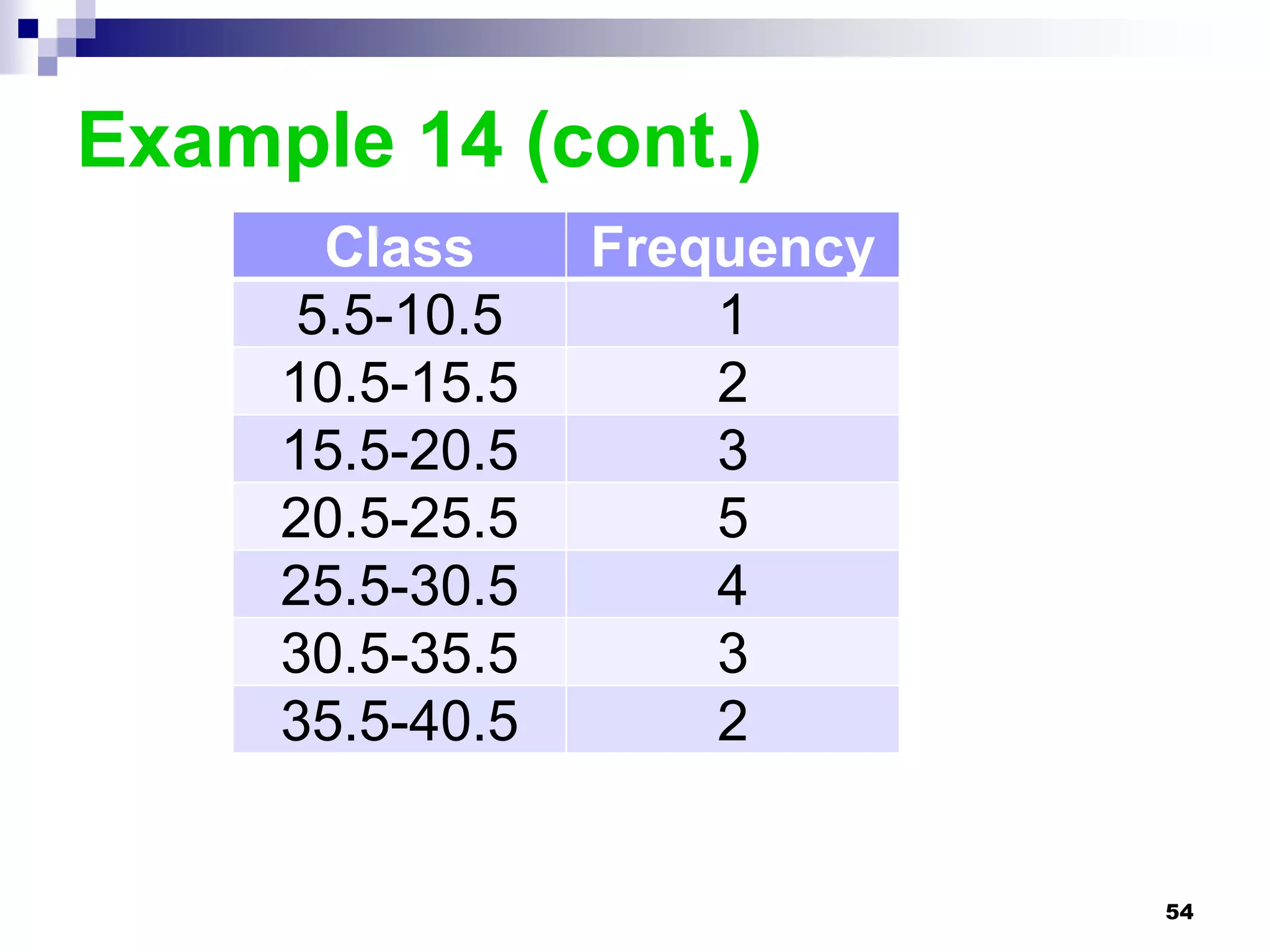
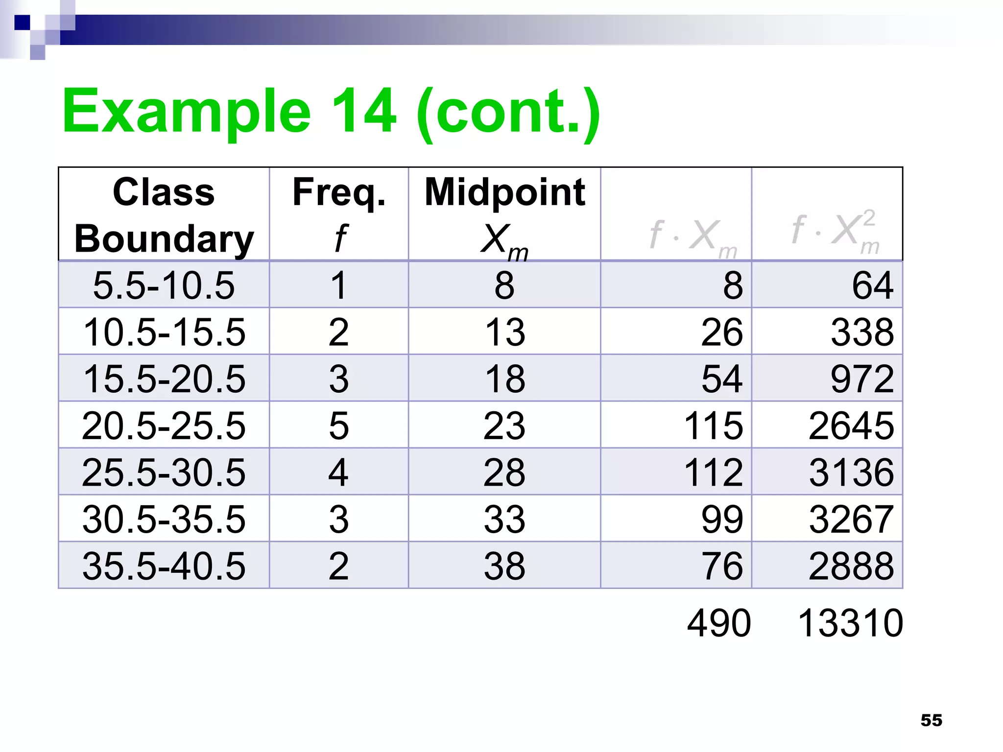
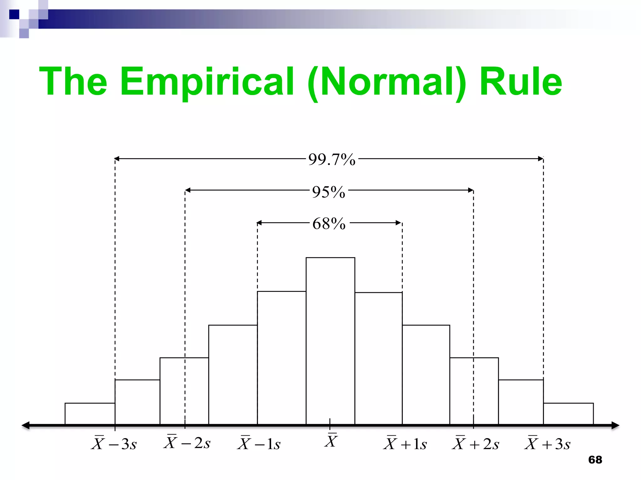
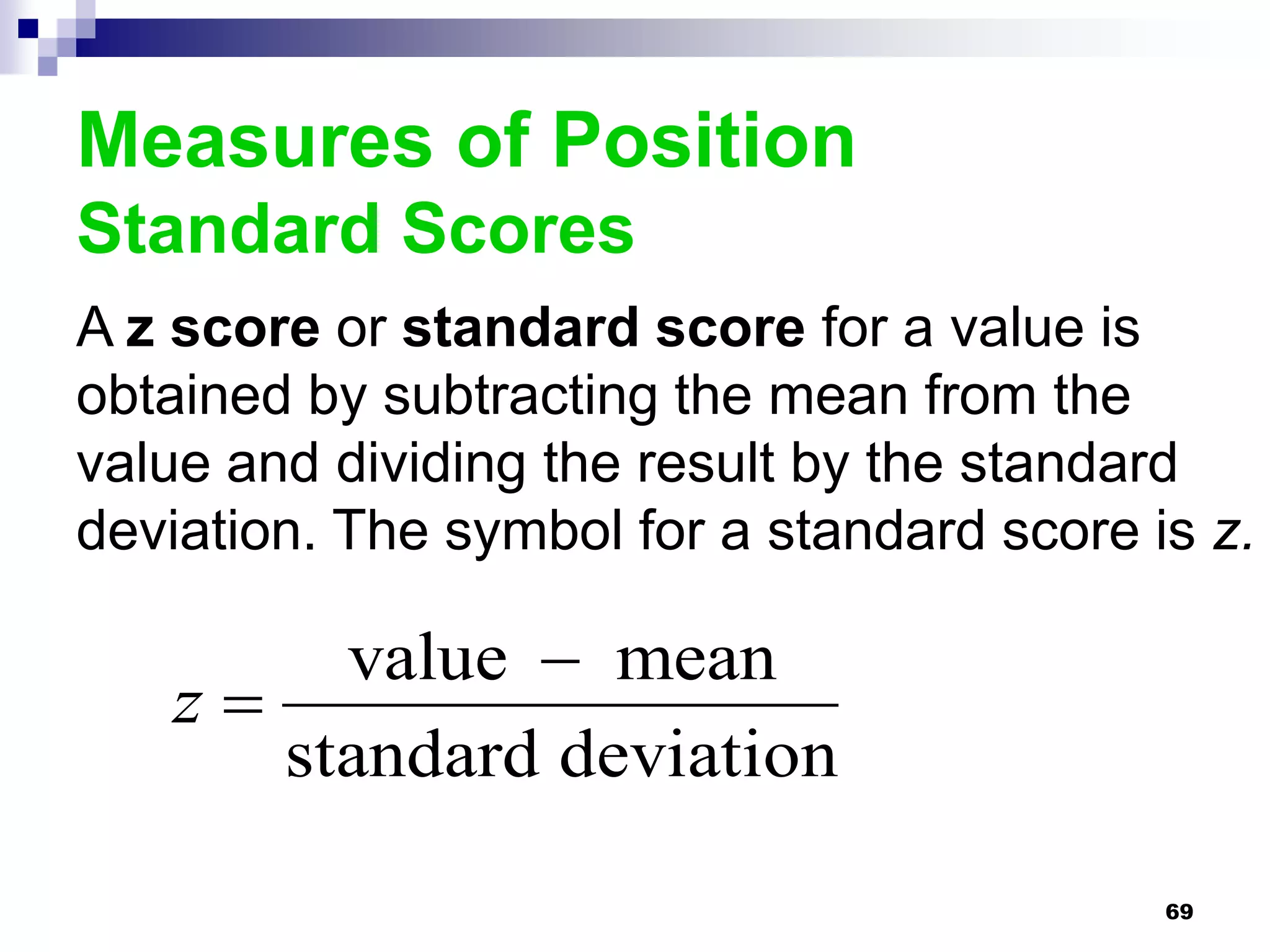
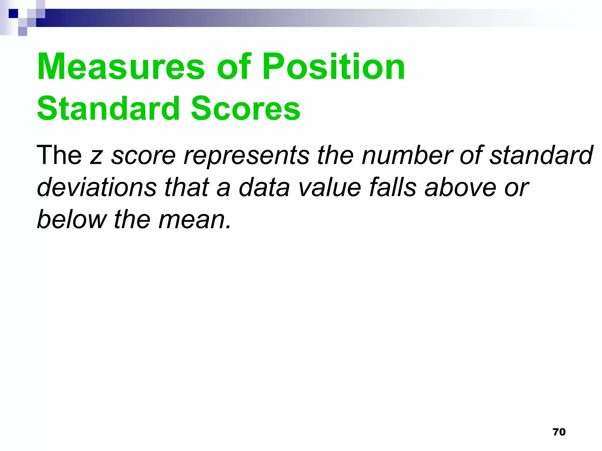
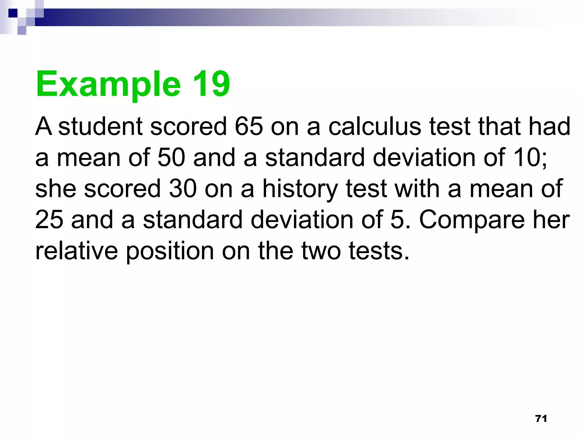
This chapter discusses measures of central tendency, dispersion, and position. It defines statistics, parameters, population and sample means, medians, modes, and weighted means. It discusses estimating means and medians for grouped data using class midpoints and boundaries. Examples are provided to demonstrate calculating measures for raw data and frequency distributions. Measures of variability like range, mean deviation, variance, and standard deviation are also introduced.

1. Chapter 3
Data Description
1

2. Through this chapter you will learn
 Measure of Central tendency
 Measure of Dispersion
 Measure of Position
2

3.  A statistic is a characteristic or measure
obtained by using the data values from a
sample.
 A parameter is a characteristic or measure
obtained by using all the data values for a
specific population.
3

4. Population Arithmetic Mean
 X
N
X : Each value, N: Total number of
values in the population
4

5. Sample Arithmetic Mean
X
X
n
X: Each value in the sample
n: Total number of observations in the
sample (sample size)
5

6. Example 1
Find the mean of the following sample data
7 4 8 8 10 12 12 .
X= 7+4+8+8+10+12+12 = 61
x
 X  61  8.71
n 7
6

7. Estimate the Mean of a Grouped
Data into a Frequency
Distribution
X
f  X m
n
f frequency of each class
Xm class midpoint of each class
n Total number of frequencies
7

8. Example 2
Given a frequency distribution
Class boundaries Frequency
5.5-10.5 1
10.5-15.5 2
15.5-20.5 3
20.5-25.5 5
25.5-30.5 4
30.5-35.5 3
35.5-40.5 2
Estimate the mean. 8

9. Example 2 (Cont.)
Midpoint
Class Frequency f fXm
5.5 - 0.5 1 8 8
10.5 - 15.5 2 13 26
15.5 - 20.5 3 18 54
20.5 - 25.5 5 23 115
25.5 - 30.5 4 28 112
30.5 - 35.5 3 33 99
35.5 - 40.5 2 38 76
total n =f= 20 f Xm= 490 9

10. Example 2 (Cont.)
X
f  X m

490
 24.5
n 20
10

11. Median
A median is the midpoint of the data array.
Steps in finding the median of a data array:
 Step1: Arrange the data in order
 Step2: Select the midpoint of the
array as the median.
11

12. Example 3
Find the median of the scores 7 2 3 7 6
9 10 8 9 9 10.
Arrange the data in order to obtain
2 3 6 7 7 8 9 9 9 10 10
We have 11 values. 8 is the exact middle
value and hence it is the median.
12

13. Example 4
Find the median of the scores 7 2 3 7 6
9 10 8 9 9
Arrange the data in order
2 3 6 7 7 8 9 9 9 10
With these ten scores, no single score is at the
exact middle. Instead, the two scores of 7 and
8 share the middle. We therefore find the
mean of these two scores. 13

14. Example 4 (Cont.)
78
 7.5
2
the median is 7.5.
14

15. The Estimate of Data Grouped
into a Frequency Distribution
n
 CF
Median  LB  2 W
f
15

16. LB Lower boundary of the median class
n Total # of frequencies
f frequency of the median class
CF Cumulative frequency of the class
preceding the median class.
w class width
16

17. Example 5
Given the frequency distribution as below.
Estimate the median.
Class Frequency
30-39 4
40-49 6
50-59 8
60-69 12
70-79 9
80-89 7
90-99 4
17

18. Example 5
First find the cumulative frequency
Class Frequency CF
30-39 4 4
40-49 6 10
50-59 8 18
60-69 12 30
70-79 9 39
80-89 7 46
90-99 4 50
18

19. Example 5
w = 10, n = 50, and hence, n/2=25. The
median falls in the class 60-69 ( 59.5-69.5)
n
 CF
Median  LB  2 W
f
25  18
 59.5   10  65.33
12
19

20. Example 6
Estimate the median for the frequency
distribution below
Class Frequency
80-89 5
90-99 9
100-109 20
110-119 8
120-129 6
130-139 2
20

21. Mode
o For grouped data into a frequency
distribution, the estimate of mode can be
the class midpoint of the modal class ( the
class with the highest frequency)
o It can also be found by the formula
d1
Mode  LB  w
d1  d 2
21

22. where
o LB Lower boundary of the modal class
o W class width
o d1 difference between class frequency of
the modal class and that of the class
preceding it.
o d2 difference between class frequency of
the modal class and that of the class right
after it.
22

23. Example 7
Estimate the mode of the below
distribution
A B
Class Frequency ( f )
5.5-10.5 1
10.5-15.5 2
15.5-20.5 3
20.5-25.5 5 Modal class
25.5-30.5 4
30.5-35.5 3
35.5-40.5 2 23

24. Example 7 (cont.)
LB = 20.5
W=5
d1= 5 - 3 =2
d2 = 5 – 4=1
2
Mode  20.5  5  23.83
2 1
24

25. The Midrange
lowest value  highest value
MR 
2
25

26. Example 8
The midrange of this data set: 2, 3, 6, 8, 4, 1
is
MR=(8+1)/2=4.5
26

27. The Weighted Mean
n
w1X1  w 2 X2    w n Xn w X i i
X  i1
w1  w 2    w n n
w
i1
i
Xi : the values
Wi : the weights
27

28. Example 8
A student obtained 40, 50, 60, 80, and 45
marks in the subjects of Math, Statistics,
Physics, Chemistry and Biology
respectively. Assuming weights 5, 2, 4, 3,
and 1 respectively for the above mentioned
subjects. Find Weighted Arithmetic Mean
per subject.
28

29. Example 8 (cont.)
Marks
Subjects Obtained Weight wx
Math 40 5 200
Statistics 50 2 100
Physics 60 4 240
Chemistry 80 3 240
Biology 55 1 55
Total 15 835
29

30. Example 8 (cont.)
835
x  55.667marks / subject
15
30

31. Distribution Shapes
y
x
Mode Median Mean
a  Positively skewed or right-skewed
31

32. Distribution Shapes (cont.)
y
x
Mean Median Mode
 b Negatively skewed or left-skewed
32

33. Distribution Shapes (cont.)
y
x
Mean = Median = Mode
33

34. Range
The range is the highest value minus the
lowest value. The symbol R is used for the
range.
R  highest value  lowest value
34

35. Mean Deviation
Mean Deviation 
 X X
n
35

36. Example 9
The number of patients seen in the
emergency room in a hospital for a sample
of 5 days last year was: 103, 97, 101, 106,
and 103. Determine the mean deviation and
interpret.
36

37. Example 9
First find the arithmetic mean
103  97  101  106  103
X  102
5
37

38. Example 9 (Cont.)
Number Absolute
Deviation
of cases Deviation
103 103 - 102= 1 1
97 97 - 102= -5 5
101 101 - 102= -1 1
106 106 - 102= 4 4
103 103 - 102= 1 1
Total 12
38

39. Example 9 (Cont.)
XX 12
MD    2.4
n 5
Hence the mean deviation is 2.4 patients per
day. The number of patients deviates, on
average, by 2.4 patients from the mean of
102 patients per day.
39

40. Example 10
The weight of a group of crates being
shipped to Ireland is (in pounds)
95, 103, 105, 110, 104, 105, 112, and 90.
a) What is the range of the weights?
b) Compute the arithmetic mean weight.
c) Compute the mean deviation of the
weights. (answer: a) 22, b) 103, c) 5.25
pounds)
40

41. Population Variance and
Standard Deviation
 X   
2
 2

N
X   
2

N
Remember: Standard deviation is the
positive square root of variance.
41

42. Example 11
Find the variance and standard deviation for
the population data: 35, 45, 30, 35, 40, 25
Solution
First find the arithmetic mean
X= 35+ 45+ 30+ 35+40+25=210
 = 210/6 = 35
then construct the table
42

43. Example 11(cont.)
X X  
2
X
35 0 0
45 10 100
30 -5 25
35 0 0
40 5 25
25 -10 100
43

44. Example 11(cont.)
The population variance is
 X   
2
250
 2
   41.7
N 6
The population standard deviation is
X   
2
  41.7  6.5
N
44

45. Sample Variance and
Standard Deviation
Sample Variance (Conceptual formula)
 X  X 
2
s 2

n 1
Sample Variance (Computational formula)
 X   X 
2 2
n
s2 
n 1
45

46. Sample Variance and
Standard Deviation (Cont.)
Sample Standard Deviation (Conceptual
formula)
 X  X 
2
s
n 1
Sample Standard Deviation (Computational
formula)
 X   X 
2 2
n
s
n 1
46

47. Example 12
Find the sample variance and standard
deviation for the amount of European auto
sales for a sample of 6 years shown. The
data are in millions of dollars.
11.2, 11.9, 12.0, 12.8, 13.4, 14.3
47

48. Example 12 (Cont.)
Method 1
Find the mean : 12.6
x  
2
X x
11.20 -1.40 1.96
11.90 -0.70 0.49
12.00 -0.60 0.36
12.80 0.20 0.04
13.40 0.80 0.64
14.30 1.70 2.89
Total= 6.38
48

49. Example 12 (Cont.)
Method 1
The variance is defined by
6.38
s 
2
 1.28
6 1
and hence, the standard deviation is
s  1.28  1.13
49

50. Example 12 (Cont.)
Method 2
We compute
X= 11.2+11.9+12.0+12.8+13.4+14.3 =75.6
X2= 11.22 +11.92 +12.02 +12.82
+13.42 +14.32 =958.94
The variance is computed by
s 
2  
958.94  75.62 6
 1.28
5
Standard deviation is 1.13
50

51. Example 13
Suppose the number of minutes you spent
for traveling to school on last 7 days are
9, 12, 9, 15, 10, 11, 15. Find the variance of
the number of minutes by the two formula.
51

52. Variance and Standard
Deviation for Grouped Data
f  X   f  Xm  n
2 2
s 2
 m
n 1
f : class frequency
Xm : class midpoint (class mark)
n : Total number of frequencies
52

53. Example
Find the variance and the standard deviation
for the frequency distribution of the data
representing the number of miles that 20
runners ran during one week.
53

54. Example 14 (cont.)
Class Frequency
5.5-10.5 1
10.5-15.5 2
15.5-20.5 3
20.5-25.5 5
25.5-30.5 4
30.5-35.5 3
35.5-40.5 2
54

55. Example 14 (cont.)
Class Freq. Midpoint
Boundary f Xm f  Xm f  Xm2
5.5-10.5 1 8 8 64
10.5-15.5 2 13 26 338
15.5-20.5 3 18 54 972
20.5-25.5 5 23 115 2645
25.5-30.5 4 28 112 3136
30.5-35.5 3 33 99 3267
35.5-40.5 2 38 76 2888
490 13310
55

56. Example 14 (cont.)
Hence, the variance is
13310  490 20 2
s 
2
20  1
 68.7
and the standard deviation is 8.3
56

57. Coefficient of Variation
The coefficient of variation is the standard
deviation divided by the mean. The result is
expressed as a percentage.

CVar   100%

s
CVar   100%
X
57

58. Example 15
The mean of the number of sales of cars over
a 3-month period is 87, and the standard
deviation is 5. The mean of the commissions
is $5225, and the standard deviation is $773.
Compare the variations of the two.
58

59. Example 15 (Cont.)
Sales
s 5
CVar    100%  5.7%
X 87
Commissions
773
CVar   100%  14.8%
5225
Since the coefficient of variation is larger for
commission, the commissions are more
variable than the sales.
59

60. Example 16
The mean for the number of pages of women’s
fitness magazines is 132, with a variance of 23;
the mean for the number of advertisements of
a sample of women’s fitness magazines is 182,
with a variance of 62. Compare the variances.
(answer: 3.6% pages, 4.3% advertisements)
60

61. Chebyshev’s theorem
The proportion of values from a data set that
will fall within k standard deviations of the
mean will be at least 1-1/k2, where k is a
number greater than 1 (k is not necessarily an
integer).
61

62. Chebyshev’s theorem
At least
88.89%
At least
75%
X  3s X  2s X X  2s X  3s
62

63. Example 17
The mean price of houses in a certain
neighborhood is $50,000, and the standard
deviation is $10, 000. Find the price range
for which at least 75% of the houses will sell.
63

64. Example 17 (Cont.)
Chebyshev’s theorem states that three-fourths,
or 75%, of the data values will fall within 2
standard deviations of the mean. Thus,
$50,000  2 $10,000  $70,000
and
$50,000  2 $10,000  $30,000
Hence, at least 75% of all homes sold in the
area will have a price range from $30,000 to
$70,000.
64

65. Example 18
A survey of local companies found that the
mean amount of travel allowance for
executives was $0.25 per mile. The standard
deviation was $ 0.02. Using Chebyshev’s
theorems find the minimum percentage of the
data values that will fall between $0.20 and
$0.30.
65

66. The Empirical (Normal) Rule
Chebyshev’s theorem applies to any
distribution regardless of its shape.
However, when a distribution is bell-shaped
(or what is called normal), the following
statements, which make up the empirical
rule, are true.
66

67. The Empirical (Normal) Rule
 Approximately 68% of the data values will
fall within 1 standard deviation of the mean.
 Approximately 95% of the data values will
fall within 2 standard deviations of the mean.
 Approximately 99.7% (almost all) of the data
values will fall within 3 standard deviations of
the mean.
67

68. The Empirical (Normal) Rule
99.7%
95%
68%
X  3s X  2s X  1s X X  1s X  2s X  3s
68

69. Measures of Position
Standard Scores
A z score or standard score for a value is
obtained by subtracting the mean from the
value and dividing the result by the standard
deviation. The symbol for a standard score is z.
value  mean
z
standard deviation
69

70. Measures of Position
Standard Scores
The z score represents the number of standard
deviations that a data value falls above or
below the mean.
70

71. Example 19
A student scored 65 on a calculus test that had
a mean of 50 and a standard deviation of 10;
she scored 30 on a history test with a mean of
25 and a standard deviation of 5. Compare her
relative position on the two tests.
71

72. Example 19 (Cont.)
For calculus, the z score is
X  X 65  50
z   1.5
s 10
For history the z score is
X  X 30  25
z   1.0
s 5
Since the z score for calculus is larger, her
relative position in the calculus class is higher
than her relative position in the history class.
72

73. Percentiles
Percentiles divide the data set into 100 equal
groups.
There are several mathematical methods for
computing percentiles for data. These
methods can be used to find approximate
percentile rank of a data value or to find a
data value corresponding to a given
percentile.
73

74. Find a Percentile Rank
Corresponding to a Value
The percentile corresponding to a given value
X is computed by using the following formula
 # of values 
   0.5
Percentile   below X   100%
total # of value
74

75. Example 20
A teacher gives a 20-point test to 10 students.
The scores are shown here. Find the
percentile rank of a score of 12.
18, 15, 12, 6, 8, 2, 3, 5, 20, 10
75

76. Example 20 (Cont.)
Arrange the data in order from lowest to highest
2, 3, 5, 6, 8, 10, 12, 15, 18, 20
6  0.5
Percentile   100%
10
 65th percentile
Thus, a student whose score was 12 did better
than 65% of the class.
76

77. Finding a Data Value Corresponding
to a Given Percentile
oArrange the data in order from lowest to highest.
oCompute c=(np)/100, where n is the total number of
observations and p the percentile.
oIf c is not a whole number, round up to the next
whole number. Starting at the lowest value, count
over to the number that corresponds to the rounded-
up value.
oIf c is a whole number, use the value halfway
between the cth and (c+1)th values when counting up
from the lowest value.
77

78. Example 21
A teacher gives a 20-point test to 10 students.
The scores are shown here. find the value
corresponding to the 25th percentile.
18, 15, 12, 6, 8, 2, 3, 5, 20, 10
78

79. Example 21 (Cont.)
oArrange the data in order from lowest to
highest
2, 3, 5, 6, 8, 10, 12, 15, 18, 20
o n= 10, p = 25
c= 10×25 / 100=2.5
o We round it up to get c =3. Start at the lowest
values and count over to the third value,
which is 5. Hence, the value 5 corresponds to
the 25th percentile.
79

80. Example 22
A teacher gives a 20-point test to 10 students.
The scores are shown here. find the value
corresponding to the 60th percentile.
18, 15, 12, 6, 8, 2, 3, 5, 20, 10
80

81. Example (22 Cont.)
o Arrange the data in order from smallest to
largest
2, 3, 5, 6, 8, 10, 12, 15, 18, 20
on= 10, p = 60
c= 10×60 / 100=6
oSince is a whole number, we use the value
halfway between the 6th and 7th values when
counting up from the lowest value
oThe 60th percentile is (10+12)/2=11.
81

82. Quartiles
Quartiles divide the distribution into 4 equal
groups, separated by Q1, Q2, and Q3.
L Q1 Q2 Q3 H
25% 25% 25% 25%
82

83. Quartiles
Quartiles can be computed using the formula
for computing percentiles.
o1st quartile corresponds to 25th percentile .
o2nd quartile corresponds to 50th percentile.
o3rd quartile corresponds to 75th percentile.
2nd quartile = 25th percentile = median
83

84. Example 23
Find first quartile, second quartile and third
quartile for the data set 15, 13, 6, 5, 12, 50,
22, 18.
Arrange the data in order from smallest to the
largest.
5 6 12 13 15 18 22 50
84

85. Example 23 (Cont.)
oFirst quartile = 25th percentile.
c = (825)/100=2
Hence, the first quartile is equal to the
second value plus the third value divided
by 2. That is,
Q1 = (6+12)/2=9
oSecond quartile = 50th percentile
c=(8 50)/100=4
Hence, Q2 =(4th value+5th value)/2
=(13+15)/2=14 85

86. Example 23 (Cont.)
oThird quartile = 75th percentile
c=(8 75)/100=6
Hence, Q3 =(6th value+7th value)/2
=(18+22)/2=20
86

87. Interquartile Range, Quartile
Deviation and Midquartile
Range
oInterquartile Range: IQR  Q3  Q1
oQuartile deviation: QD (Q3  Q1)/2
oSemi-interquartile range is referred to
quartile deviation.
oMidquartile Range : (Q3  Q1)/2
87

88. Quartiles of Data Grouped
into a Freq. Dist.
oFirst quartile
n / 4  CF
Q1  LB  w
f
oSecond quartile (Median)
n / 2  CF
Q2  LB  w
f
oThird quartile
3n / 4  CF
Q3  LB  w
f 88

89. Example 24
The office manager of the Mallard Glass Co.
is investigating the ages in months of the
company’s PCs currently in use. The ages of
30 units selected at random were organized
into a frequency distribution. Compute the
quartile deviation.
89

90. Example 24 (Cont.)
Age
(in months) # of PCs
20-24 3
25- 29 5
30-34 10
35-39 7
40-44 4
45-49 1
90

91. Example 24 (Cont.)
Age Cumu.
(in months) # of PCs Freq.
20-24 3 3
25- 29 5 8
30-34 10 18
35-39 7 25
40-44 4 29
45-49 1 30
91

92. Example 24 (Cont.)
30 / 4  3
Q1  24.5   5  29
5
3  30 / 4  18
Q2  35.5  5
7
 38.71
Hence, QD 38.7129  4.855 months
92

93. Example 25
The weekly income of a sample of 60 part
time employees of a fast-food restaurant
chain was organized into the following
frequency distribution. Compute the
standard deviation and quartile deviation.
93

94. Example 25 (Cont.)
Weekly Number of
Incomes Employees
100-149 5
150-199 9
200-249 20
250-299 18
300-349 5
350-399 3
94

95. Outliers
 An outlier is an extremely high or an
extremely low data value when compared
with the rest of the data values.
 An outlier can strongly affect the mean
and standard deviation of a variable.
 There are several ways to check a data
set for outliers. One of which is shown as
follows:
95

96. Outliers (Cont.)
Step1 Arrange the data in order and find Q1
and Q3.
Step2 Find the inter-quartile range:
IQR=Q3 Q1
Step3 Multiply the IQR by 1.5.
Step5 Check the data set for any data value
which is smaller than Q11.5IQR or
larger than Q3 1.5IQR .
96

97. Outliers: Example 26
Check the following data set for outliers.
5, 6, 12, 13, 15, 18, 22, 50
We found Q19, Q320
Inter-quartile Range: IQR 20-9=11
Compute the dividing points:
Q11.5IQR 91.5117.5
Q3 1.5IQR 201.51136.5
The data value of 50 is greater than the
upper dividing point of 36.5. So, the data
value of 50 is considered an outlier.
97

98. Exploratory Data Analysis
oIn exploratory data analysis (EDA) the
data are presented graphically using a box-
plot (sometimes called a box-and-whisker
plot).
oThe purpose of exploratory data analysis is
to examine data to find out what information
can be discovered about the data such as
the center and the spread.
oEDA was developed by John Tukey.
98

99. Exploratory Data Analysis
A box plot can be used to graphically
represent the data set. These plots involve five
specific values:
o The lowest value (i.e., minimum)
o Q1
o Median (Q2)
o Q3
o The highest value (i.e., maximum)
99

100. Example 27 (Box-plot)
A stockbroker recorded the number of clients
she saw each day over an 11-day period the
data are shown below. Construct a box plot
for the data.
33, 38, 43, 30, 29, 40, 51, 27, 42, 23, 31
100

101. Example 27 (Box-plot)
oArrange the data in order from lowest to the
highest:
23, 27, 29, 30, 31, 33, 38, 40, 42, 43, 51
oWe obtain: the lowest value23, Q129,
Median  Q2  33, Q3 43, and the highest
value 15.
29 33 42
23 51
20 25 30 35 40 45 50 101

102. THE END!
102