1. Chapter 7
Problem Solutions
7.1
a.
V0 ( s ) 1/ ( sC1 )
T (s) = =
Vi ( s ) ⎡1/ ( sC1 ) ⎤ + R1
⎣ ⎦
1
T (s) =
1 + sR1C1
b.
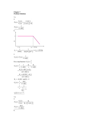
1
͉T ͉
f fH ϭ 159 Hz
1 1
fH = = ⇒ f H = 159 Hz
2π R1C1 2π (103 )(10−6 )
c.
1
V0 ( s ) = Vi ( s ) ⋅
1 + sR1C1
1
For a step function Vi ( s ) =
s
1 1 K K2
V0 ( s ) = ⋅ = 1+
s 1 + sR1C1 s 1 + sR1C1
K1 (1 + sR1C1 ) + K 2 s
=
s (1 + sR1C1 )
K1 + s ( K1 R1C1 + K 2 )
=
s (1 + sR1C1 )
K 2 = − K1 R1C1 and K1 = 1
1 − R1C1
V0 ( s ) = +
s 1 + sR1C1
1 1
= −
s 1
+s
R1C1
v0 ( t ) = 1 − e− t / R1C1
7.2
a.
V0 ( s ) R2
T (s) = =
Vi ( s ) R2 + ⎡1/ ( sC2 ) ⎤
⎣ ⎦
sR2 C2
T (s) =
1 + sR2 C2
b.

2. 1
͉T ͉
fL ϭ 1.59 Hz
1 1
fL = = ⇒ f L = 1.59 Hz
2π R2 C2 2π (10 )(10 × 10−6 )
4
c.
sR2 C2
V0 ( s ) = Vi ( s ) ⋅
1 + sR2 C2
1
Vi ( s ) =
s
R2 C2 1
V0 ( s ) = =
1 + sR2 C2 s + 1
R2 C2
v0 ( t ) = e− t / R2C2
7.3
a.
1
RP
V0 ( s ) sCP
T (s) = =
Vi ( s ) 1 ⎛ 1 ⎞
RP + ⎜ RS + ⎟
sCP ⎝ sCS ⎠
1
RP ⋅
1 sCP RP
RP = =
sCP R + 1 1 + sRP CP
P
sCP
Then
RP
T (s) =
⎛ 1 ⎞
RP + ⎜ RS + ⎟ (1 + sRP CP )
⎝ sCS ⎠
RP
=
RP CP 1
RP + RS + + + sRS RP CP
CS sCS
⎛ RP ⎞ ⎛ ⎡ RP C 1 sRP RS ⎤⎞
T (s) = ⎜ ⎟ × ⎜ 1/ ⎢1 + ⋅ P+ + ⋅ CP ⎥ ⎟
⎝ RP + RS ⎠ ⎜ ⎢ RP + RS CS s ( RS + RP ) CS RS + RP
⎝ ⎣ ⎥⎟
⎦⎠
b.

3. ⎛ ⎤⎞
⎛ 10 ⎞ ⎜ ⎡ 10 10
−11
+ s ( 5 × 103 ) ⋅10−11 ⎥ ⎟
1
T (s) = ⎜ ⎟ × 1/ ⎢1 + ⋅ −6 +
⎝ 10 + 10 ⎠ ⎜ ⎢ 20 10 s ( 2 × 104 ) ⋅10−6 ⎥⎟
⎝ ⎣ ⎦⎠
1 1
≅ ⋅
+ s ( 5 × 10−8 )
2 1+ 1
s ( 0.02 )
s = jω
1 1
T ( jω ) = ⋅
2 ⎡ ⎤
1 + j ⎢ω ( 5 × 10−8 ) −
1
⎥
⎣ ω ( 0.02 ) ⎦
1 1
For ω L = = = 50
( RS + RR ) CS ( 2 ×10 )(10−6 )
4
1 1
T ( jω ) = ⋅
2 ⎡ ⎤
1 + j ⎢( 50 ) ( 5 × 10−8 ) −
1
⎣ ( 50 )( 0.02 ) ⎥
⎦
1 1 1 1
≈ ⋅ ⇒ T ( jω ) = ⋅
2 1− j 2 2
For
1 1
ωH = = = 2 × 107
( RS RP ) CP ( 5 × 103 )(10−11 )
1 1
T ( jω ) = ⋅
2 ⎡ ⎤
1 + j ⎢( 2 × 107 )( 5 × 10−8 ) −
1
⎥
⎢
⎣ ( 2 ×107 ) ( 0.02 ) ⎥
⎦
1 1 1 1
T ( jω ) ≈ ⋅ ⇒ T ( jω ) = ⋅
2 1+ j 2 2
1 RP
In each case, T ( jω ) = ⋅
2 RP + RS
c.
RS = RP = 10 kΩ, CS = CP = 0.1 μ F
⎛ ⎡ ⎤⎞
+ s ( 5 × 103 )(10−7 ) ⎥ ⎟
1 ⎜ ⎢ 1 1 1
T (s) = ⋅ 1/ 1 + ⋅ +
⎜
⎝ ⎣ (
2 ⎜ ⎢ 2 1 s 2 × 104 (10−7 ) ) ⎥⎟
⎦⎠
⎟
s = jω
1 1
T ( jω ) = ⋅
2 ⎡ ⎤
1 + + j ⎢ω ( 5 × 10−4 ) −
1 1
⎥
2 ⎢
⎣ ω ( 2 × 10−3 ) ⎥
⎦
1
For ω = = 500
( 2 ×104 )(10−7 )
1 1
T ( jω ) = ⋅
2 ⎡ ⎤
1.5 + j ⎢( 500 ) ( 5 × 10−4 ) −
1
⎥
⎢
⎣ ( 500 ) ( 2 ×10−3 ) ⎥
⎦
1 1
= ⋅ ⇒ T ( jω ) = 0.298
2 1.5 − j ( 0.75 )

4. 1
For ω = = 2 × 103
( 5 ×10 )(10 )
3 −7
⎧ ⎛ ⎡ ⎫
⎤ ⎞⎪
1 ⎪ ⎜
⋅ ⎨1/ 1.5 + j ⎢( 2 × 103 )( 5 × 10−4 ) −
1
T ( jω ) = ⎥ ⎟⎬
2 ⎪ ⎜
⎩ ⎝
⎢
⎣ ( 2 ×103 )( 2 ×10−3 ) ⎥ ⎟⎪
⎦ ⎠⎭
1 1
= ⋅ ⇒ T ( jω ) = 0.298
2 1.5 + j ( 0.75 )
1 RP
In each case, T ( jω ) < ⋅
2 RP + RS
7.4
Circuit (a):
V R2 R2
T= 0 = =
Vi 1 R1 (1/ sC1 )
R2 + R2 +
sC1 R1 + (1/ sC1 )
R2 R2 (1 + sR1C1 ) Vo R2 (1 + sR1C1 )
= = or = ⋅
R1 R2 + sR1 R2 C1 + R1 Vi R1 + R2 1 + sR1 R2 C1
R2 +
1 + sR1C1
Low frequency:
Vo R2 20 2
= = =
Vi R1 + R2 10 + 20 3
High frequency:
Vo
=1
Vi
τ 1 = R1C1 = (104 )(10 × 10−6 ) = 0.10 ⇒ f1 =
1
= 1.59 Hz
2πτ 1
τ 2 = ( R1 R 2 ) C1 = (10 20 ) × 103 × (10 × 10−6 ) ⇒ τ 2 = 0.0667 ⇒ f 2 =
1
= 2.39 Hz
2πτ 2
͉T ͉
1.0
0.67
1.59 2.39 f
Circuit (b):
1 R2
R2
V 1 + sR2 C2
sC2
T= o = =
Vi 1 R2
R2 + R1 + R1
sC2 1 + sR2 C2
⎛ R2 ⎞ ⎛ 1 ⎞
=⎜ ⎟⎜ ⎟
⎝ R1 + R2 ⎠ ⎝ 1 + s ( R1 R2 ) C2 ⎠
⎜ ⎟
Low frequency:
Vo R2 20 2
= = =
Vi R1 + R2 20 + 10 3
τ = ( R1 R2 ) C2 = (10 20 ) × 103 × 10 × 10−6 = 0.0667
1
f = = 2.39 Hz
2πτ

5. 0.67
͉T ͉
2.39 f
7.5
a.
rS = ( Ri + RP ) CS = [30 + 10] × 103 × 10 × 10−6 ⇒ rS = 0.40 s
rP = ( Ri RP ) CP = ⎡30 10 ⎤ × 103 × 50 × 10−12 ⇒ rP = 0.375 μ s
⎣ ⎦
b.
1 1
fL = = ⇒ f L = 0.398 Hz
2π rS 2π ( 0.4 )
1 1
fH = = ⇒ f H = 424 kHz
2π rP 2π ( 0.375 × 10−6 )
At midband. CS → short, CP → open
Vo = I i ( Ri RP )
T ( s ) = Ri R P = 30 10 ⇒ T ( s ) = 7.5 k Ω
c.
7.5 k⍀
͉T ͉
fL fH
7.6
(a)
1 1 1
T= ⇒T = =
(1 + j 2π f τ )
( ) 1 + ( 2π f τ )
2 2 2
1 + ( 2π f τ )
2
T max
=1
1 1 1
At f = ⇒T = =
2πτ 1 + (1)
2
2
⎛1⎞
T = 20 log10 ⎜ ⎟ ⇒ T dB ≅ −6 dB
⎝ 2⎠
dB
Phase = 2 tan ( 2π f τ ) = −2 tan −1 (1) = −2 ( 45° ) ⇒ Phase = −90°
−1
(b)
Slope = −2 ( 6dB / oct ) = −12dB / oct = −40dB / decade
Phase = −2 ( 90° ) ⇒ Phase = −180°
7.7
(a)

6. −10 ( jω )
T ( jω ) =
⎛ jω ⎞ ⎛ jω ⎞
20 ⎜ 1 + ⎟ ( 2000 ) ⎜1 + ⎟
⎝ 20 ⎠ ⎝ 2000 ⎠
⎛ jω ⎞
−5 × 10−3 ⎜ ⎟
⎝ ω ⎠ = 2.5 × 10 ( jω )
−4
=
⎛ jω ⎞ ⎛ jω ⎞ ⎛ jω ⎞⎛ jω ⎞
⎜1 + 1+ 1+ 1+
⎝ ω ⎟ ⎜ 2000 ⎟ ⎜ 20 ⎟⎜ 2000 ⎟
⎠⎝ ⎠ ⎝ ⎠⎝ ⎠
2.5 × 10−4 (ω )
T =
⎛ω ⎞ ⎛ ω ⎞
2 2
1+ ⎜ ⎟ ⋅ 1+ ⎜ ⎟
⎝ 20 ⎠ ⎝ 2000 ⎠
͉T ͉
5 ϫ 10Ϫ3
2.5 ϫ 10Ϫ4
1 20 2000 ␻
(b)
jω ⎞
(10 )(10 ) ⎛1 +
⎜⎟
T ( jω ) = ⎝ 10 ⎠
⎛ jω ⎞
1000 ⎜ 1 + ⎟
⎝ 1000 ⎠
⎛ω ⎞
2
( 0.10 ) 1+ ⎜ ⎟
⎝ 10 ⎠
T =
⎛ ω ⎞
2
1+ ⎜ ⎟
⎝ 1000 ⎠
͉T ͉
10
0.10
10 1000 ␻
7.8
(a)
105 10 5
T (s) = = ⋅
( 5 + 10 )( 5 + 500 ) (10 )( 500 ) ⎛ 5 ⎞⎛ 5 ⎞
⎜ + 1⎟⎜ + 1⎟
⎝ 10 ⎠⎝ 500 ⎠
⎛ jω ⎞
⎜ ⎟
=
10
⋅ ⎝ 10 ⎠
500 ⎛ jω ⎞⎛ jω ⎞
⎜ + 1⎟⎜ + 1⎟
⎝ 10 ⎠⎝ 500 ⎠

7. ͉T ͉
0.02
10 500 ␻(rod/s)
(b) Midband gain = 0.02
(c) ω = 500 rad/s
(d) ω = 10 rad/s
7.9
(a)
2 × 104
T ( s) =
( S + 10 )( S + 10 )
3 5
2 × 104 1
= ⋅
(10 )(10 )
3 5
⎛ S ⎞⎛ S ⎞
⎜ 3 + 1 ⎟ ⎜ 5 + 1⎟
⎝ 10 ⎠⎝ 10 ⎠
2 × 10−4
T ( jω ) =
⎛ jω ⎞ ⎛ jω ⎞
⎜ 3 + 1 ⎟ ⎜ 5 + 1⎟
⎝ 10 ⎠ ⎝ 10 ⎠
͉T ͉
2 ϫ 10Ϫ4
10 3 10 5 ␻(rod/s)
−4
(b) 2 × 10
(c) ω = 103 rad/s
(d) no low freq −3dB freq.
7.10
a.
⎛ r ⎞
V0 = − g mVπ RL Vπ = ⎜ π ⎟ Vi
⎝ rπ + RS ⎠
⎛ r ⎞ ⎛ 5.2 ⎞
T = g m RL ⎜ π ⎟ = ( 29 )( 6 ) ⎜ ⎟
⎝ rπ + RS ⎠ ⎝ 5.2 + 0.5 ⎠
Tmidband = 159
b.
rS = ( RS + rπ ) CC
1 1 1
fL = ⇒ rS = = ⇒ rS = 5.31 ms Open-circuit
2π rS 2π f L 2π ( 30 )
1 1
rP = = ⇒ τ P = 0.332 μ s Short-circuit
2π f H 2π ( 480 × 103 )

8. c.
rS 5.31× 10−3
CC = = ⇒ CC = 0.932 μ F
( RS + τ π ) ( 0.5 + 5.2 ) ×103
rP = RL CL
rP 0.332 × 10−6
CL = = ⇒ CL = 55.3 pF
RL 6 × 103
7.11 Computer Analysis
7.12 Computer Analysis
7.13
a.
RTH = R1 R2 = 10 1.5 = 1.304 kΩ
⎛ R2 ⎞ ⎛ 1.5 ⎞
VTH = ⎜ ⎟ VCC = ⎜ ⎟ (12 ) = 1.565 V
⎝ R1 + R2 ⎠ ⎝ 1.5 + 10 ⎠
1.565 − 0.7
I BQ = = 0.0759 mA
1.30 + (101)( 0.1)
I CQ = 7.585 mA
(100 )( 0.026 )
rπ = = 0.343 kΩ
7.59
7.59
gm = = 292 mA/V
0.026
Ri = R1 R2 ⎡ rπ + (1 + β ) RE ⎤
⎣ ⎦
= 10 1.5 ⎡0.343 + (101)( 0.1) ⎤
⎣ ⎦
= 1.30 10.44 ⇒ Ri = 1.159 kΩ
r = ( RS + Ri ) CC = [ 0.5 + 1.16] × 103 × 0.1× 10−6
r = 1.659 × 10−4 s
1 1
fL = = ⇒ f L = 959 Hz
2π r 2π (1.66 × 10−4 )
b.
Rib
RS
V0
ϩ
Ib
V␲ r␲ gmV␲
ϩ Ϫ
Vi R1͉͉R2 RC
Ϫ
RE

9. V0 = − ( β I b ) RC
R1b = rπ + (1 + β ) RE
= 0.343 + (101)( 0.1) = 10.44 kΩ
⎛ R1 R2 ⎞
Ib = ⎜
⎜R R +R ⎟ i
I
⎟
⎝ 1 2 ib ⎠
⎛ 1.30 ⎞
=⎜ ⎟ I i = ( 0.111) I i
⎝ 1.30 + 10.4 ⎠
Vi
Ii =
RS + R1 R2 Rib
Vi
=
0.5 + (1.3) (10.44 )
Vi
Ii =
1.659
V0 β RC ( 0.111) V0 (100 )(1)( 0.111) V0
= ⇒ = ⇒ = 6.69
Vi 1.659 Vi midband
1.659 Vi midband
c.
6.69
͉V ͉
V
0
i
fL ϭ 959 Hz f
7.14
I DQ = 0.5 mA ⇒ VS = ( 0.5 )( 0.5 ) = 0.25 V
0.5
I DQ = K n (VGS − VTN ) ⇒ VGS =
2
+ 1.5 = 3.08 V
0.2
VG = VGS + VS = 3.08 + 0.25 ⇒ VG = 3.33 V
⎛ R2 ⎞ 1
VG = ⎜ ⎟ VDD ⇒ 3.33 = ⋅ Rin ⋅ VDD
⎝ R1 + R2 ⎠ R1
1
3.33 = ( 200 )( 9 ) ⇒ R1 = 541 kΩ
R1
541R2
= 200 ⇒ R2 = 317 kΩ
541 + R2
VD = VDSQ + VS = 4.5 + 0.25 = 4.75
9 − 4.75
RD = ⇒ RD = 8.5 kΩ
0.5
1 1 1
fL = ⇒ rL = = = 7.96 ms
2π rL 2π f L 2π ( 20 )
rL 7.96 × 10−3
rL = Rin ⋅ CC ⇒ CC = = ⇒ CC = 0.0398 μ F
Rin 200 × 103
g m = 2 ( 0.2 )( 3.08 − 1.5 ) = 0.632 mA/V
g m RD ( 0.632 )(8.5)
Av = = ⇒ Av = 4.08
midband
1 + g m RS 1 + ( 0.632 )( 0.5 )

10. 4.08
͉A␯͉
fL ϭ 20 Hz f
Phase fL
Ϫ90
Ϫ135
Ϫ180
7.15
I DQ 1
I DQ = K n (VGS − VTN ) ⇒ VGS =
2
+ VTN = + 1 = 2.414 V
Kn 0.5
VS = −2.414 V
−2.414 − ( −5 )
RS = ⇒ RS = 2.59 kΩ
1
VD = VDSQ + VS = 3 − 2.414 = 0.586 V
5 − 0.59
RD = ⇒ RD = 4.41 kΩ
1
b.
CC
ϩ
Vi ϩ RG Vgs gmVgs
Ϫ
I0
RD RL
Ϫ
RS
⎛ ⎞
⎜ ⎟
I 0 = − ( g mVgs ) ⎜
RD
⎟
⎜R +R + 1 ⎟
⎜ D L ⎟
⎝ sCC ⎠
Vi
Vgs =
1 + g m RS
I0 ( s ) − gm ⎡ sCC ⎤
= ⋅ RD ⎢ ⎥
Vi ( s ) 1 + g m RS ⎢1 + s ( RD + RL ) CC ⎥
⎣ ⎦
I0 ( s )
T (s) =
Vi ( s )
− g m RD 1 s ( RD + RL ) CC
= ⋅ ⋅
1 + g m RS RD + RL 1 + s ( RD + RL ) CC
c.

11. 1 1 1
fL = → rL = = = 15.92 ms
2π rL 2π f L 2π (10 )
rL 15.9 × 10−3
rL = ( RD + RL ) CC ⇒ CC = = ⇒ CC = 1.89 μ F
RD + RL ( 4.41 + 4 ) × 103
7.16
a.
9 − VSG
= I D = K P (VSG + VTP )
2
RS
9 − VSG = ( 0.5 )(12 ) (VSG − 4VSG + 4 )
2
6VSG − 23VSG + 15 = 0
2
( 23) − 4 ( 6 )(15 )
2
23 ±
VSG = ⇒ VSG = 3 V
2 ( 6)
g m = 2 K P (VSG + VTP ) = 2 ( 0.5 )( 3 − 2 ) ⇒ g m = 1 mA/V
1
Ro = RS = 1 12 ⇒ Ro = 0.923 kΩ
gm
b. r = ( R0 + RL ) CC
1 1 1
c. fL = ⇒r= = = 7.96 ms
2πτ 2π f L 2π ( 20 )
r 7.96 × 10−3
CC = = ⇒ CC = 0.729 μ F
Ro + RL ( 0.923 + 10 ) × 103
7.17
a.
1
I CQ = 1 mA, I BQ = = 0.00833 mA
120
R1 || R2 = ( 0.1)(1 + β )( RE )
= ( 0.1)(121)( 4 ) = 48.4 kΩ
VTH = I BQ RTH + VBE ( on ) + (1 + β ) I BQ RE
1
⋅ RTH ⋅ VCC = ( 0.00833)( 48.4 ) + 0.7 + (121)( 0.00833)( 4 )
R1
1
( 48.4 )(12 ) = 5.135
R1
R1 = 113 kΩ
113R2
= 48.4 ⇒ R2 = 84.7 k Ω
113 + R2
b.
r
R0 = π RE r0
1+ β
(120 )( 0.026 )
rπ = = 3.12 kΩ
1
80
r0 = = 80 kΩ
1
3.12
R0 = 4 80 = 0.02579 4 80 ⇒ R0 = 25.6 Ω
121
c.

12. r = ( R0 + RL ) CC 2
r = ( 0.0256 + 4 ) × 103 × 2 × 10−6 = 8.05 × 10−3 s
1 1
f = = ⇒ f = 19.8 Hz
2π r 2π ( 8.05 × 10−3 )
7.18
(a)
5 − 0.7
I EQ = = 1.075 mA I CQ = 1.064 mA
4
VCEQ = 10 − (1.064 )( 2 ) − (1.075 )( 4 )
VCEQ = 3.57 V
I CQ 1.064
gm = = = 40.92 mA/V
VT 0.026
β VT (100 )( 0.026 )
rπ = = = 2.44 K
I CQ 1.064
(b)
rπ 2440
For CC1 , Req1 = RS + RE = 200 + 4000
1+ β 101
Req1 = 224.0r , τ 1 = Req1CC1 = 1.053 ms
For CC 2 , Req 2 = RC + RL = 2 + 47 = 49 K
τ 2 = Req 2 ⋅ Cc 2 = 49 ms
1 1
(c) f1 = = ⇒ f1 = 151 Hz
2πτ 1 2π (1.053 × 10−3 )
7.19
(a)
τ H = ( RC RL ) CL = ( 2 47 ) × 103 × 10 × 10−12
= 1.918 × 10−8 s
1 1
fH = = ⇒ f H = 8.30 MHz
2πτ H 2π (1.918 × 10−8 )
(b)
1
= 0.1
1 + ( f .2πτ H )
2
2
⎛ 1 ⎞
⎟ = 100 = 1 + ( f .2πτ H )
2
⎜
⎝ 0.1 ⎠
99 99
f = =
2πτ H 2π (1.918 × 10−8 )
f = 82.6 MHz
7.20
(a)

13. 5 − VSG
= K P (VSG + VTP )
2
R1
5 − VSG = (1)(1.2 )(VSG − 1.5 ) = (1.2 ) (VSG − 3VSG + 2.25 )
22
1.2VSG − 2.6VSG − 2.3 = 0⇒ VSG = 2.84 V
2
I DQ = 1.8 mA
VSDQ = 10 − (1.8 )(1.2 + 1.2 ) ⇒ VSDQ = 5.68 V
g m = 2 K P I DQ = 2 (1)(1.8 ) = 2.683 mA / V
ro = ∞
(b)
1 1
Ris = = = 0.3727 k Ω
g m 2.68
Ri = 1.2 0.373 = 0.284 k Ω
For CC1 , τ s1 = ( 284 + 200 ) ( 4.7 × 10−6 ) = 2.27 ms
For CC 2 , τ s 2 = (1.2 x103 + 50 × 103 )(10−6 ) = 51.2 ms
(c)
CC2 dominates,
1 1
f 3− dB = = = 3.1 Hz
2πτ s 2 2π ( 51.2 × 10−3 )
7.21
′
Assume VTN = 1V , kn = 80μ A / V 2 , λ = 0
Neglecting RSi = 200Ω , Midband gain is:
Av = g m RD
Let I DQ = 0.2 mA, VDSQ = 5V
9−5
Then RD = ⇒ RD = 20 k Ω
0.2
Av 10 ⎛ k′ ⎞⎛ W ⎞
We need g m = = = 0.5 mA / V 2 and g m = 2 K n I DQ = 2 ⎜ n ⎟ ⎜ ⎟ I DQ
RD 20 ⎝ 2 ⎠⎝ L ⎠
⎛ 0.080 ⎞ ⎛ W ⎞ W
or 0.5 = 2 ⎜ ⎟ ⎜ ⎟ ( 0.2 ) ⇒ = 7.81
⎝ 2 ⎠⎝ L ⎠ L
Let
9 9
R1 + R2 = = = 225 k Ω
( 0.2 ) I DQ ( 0.2 )( 0.2 )
⎛ 0.080 ⎞ ⎛ R2 ⎞ ⎛ R2 ⎞
⎟ ( 7.81)(VGS − 1) ⇒ VGS = 1.80 = ⎜ ⎟ (9 ) = ⎜ ⎟ (9) ⇒
2
I DQ = 0.2 = ⎜
⎝ 2 ⎠ ⎝ R1 + R2 ⎠ ⎝ 225 ⎠
R2 = 45 k Ω, R1 = 180 k Ω
RTH = R1 R2 = 180 45 = 36 k Ω
1 1 7.96 × 10−4
τ1 = = = 7.958 × 10−4 s = ( RSi + RTH ) CC or CC = ⇒
2π f1 2π ( 200 ) ( 200 + 36 ×103 )
CC = 0.022 μ F
1 1 5.31× 10−5
τ2 = = = 5.305 × 10−5 s = RD CL or CL = ⇒ CL = 2.65 nF
2π f 2 2π ( 3 x103 ) 20 × 103
7.22
a.

14. R2 + (1/ sC )
T (s) =
R2 + (1/ sC ) + R1
1 + sR2 C
T (s) =
1 + s ( R1 + R2 ) C
rA = R2 C , rB = ( R1 + R2 ) C
b.
͉T ͉
1
0.0909
fB fA f
c.
rA = R2 C = (103 )(100 × 10−12 ) = 10−7 s = rA
rB = ( R1 + R2 ) C = [10 + 1] × 103 × 100 × 10−12
= 1.1× 10−6 s = rB
1 1
fA ≈ = ⇒ f A = 1.59 MHz
2π rA 2π (10−7 )
1 1
fB ≈ = ⇒ f B = 0.145 MHz
2π rB 2π (1.1× 10−6 )
7.23
10 − 0.7
I BQ = = 0.00997 mA
430 + ( 201)( 2.5 )
I CQ = ( 200 ) I BQ = 1.995 mA
( 200 )( 0.026 )
rπ = = 2.61 k Ω
1.99
Rib = 2.61 + ( 201)( 2.5 ) = 505 k Ω
1 1
τs = = = 0.0106 s
2π f L 2π (15 )
= Req CC = ( 0.5 + 505 430 ) × 103 CC = 232.7 × 103 CC
Or CC = 4.55 × 10−8 F ⇒ 45.5 nF
7.24
10 = I BQ (300) + 0.7 + ( 201) I BQ (1) ⇒ I BQ = 0.0186 mA ⇒ I CQ = 3.7126 mA
β VT ( 200 )( 0.026 )
rπ = = = 1.40 K
I CQ 3.71
Ri = rπ + (1 + β ) RE = 1.40 + ( 201)(1) = 202.4 K
Req = RS + RB Ri = 0.1 + 300 202.4 = 121 K
τ L = Req ⋅ CC
1 1 1
fL = ⇒τL = = = 7.958 × 10−3 s
2πτ L 2π f 2π ( 20 )
τL 7.958 × 10−3
CC = = ⇒ CC = 0.0658 μ F
Req 121× 103
7.25

15. RTH = R1 R2 = 1.2 1.2 = 0.6 k Ω
⎛ R2 ⎞ ⎛ 1.2 ⎞
VTH = ⎜ ⎟ (VCC ) = ⎜ ⎟ ( 5 ) = 2.5 V
⎝ R1 + R2 ⎠ ⎝ 1.2 + 1.2 ⎠
2.5 − 0.7
I BQ = = 0.319 mA
0.6 + (101)( 0.05 )
I CQ = 31.9 mA
(100 )( 0.026 )
rπ = = 0.0815 k Ω
31.9
1
τ C >> τ C and f = so that f 3− dB ( CC1 ) << f3− dB ( CC 2 )
C1 C2
2πτ
Then, for f 3− dB ( CC1 ) ⇒ CC 2 acts as an open and for f 3− dB ( CC 2 ) ⇒ CC1 acts as a short circuit.
1 1
f 3− dB ( CC 2 ) = 25 Hz = , so that τ 2 = = 0.006366 s = Req CC 2
2πτ 2 2π ( 25 )
where
⎛ r + R1 R2 RS ⎞
Req = RL + RE ⎜ π ⎟
⎝ 1+ β ⎠
⎛ 81.5 + 600 300 ⎞
= 10 + 50 ⎜ ⎟ = 10 + 50 2.787 ⇒
⎝ 101 ⎠
0.00637
Req = 12.64 Ω ⇒ CC 2 = ⇒ CC 2 = 504 μ F
12.6
Rib = rπ + (1 + β ) RE Assume CC 2 an open
Rib = 81.5 + (101)( 50 ) = 5132 Ω
τ 1 = (100 )τ 2 = (100 )( 0.006366 ) = 0.6366 s = Req1CC1
Req1 = RS + RTH Rib = 300 + 600 5132 = 837.2 Ω
0.6366
So CC1 = ⇒ CC1 = 760 μ F
837.2
7.26
From Problem 7.25 RTH = 0.6 K, I CQ = 31.9 mA, rπ = 81.5 Ω
1
τC2 τ C1 and f = so f 3− dB ( CC 2 ) f 3− dB ( CC1 )
2πτ
Then f 3− dB ( CC 2 ) ⇒ CC1 acts as an open circuit and for f 3− dB ( CC1 ) ⇒ CC 2 acts as a short circuit.
1
f 3− dB ( CC1 ) = 20 Hz = ⇒ τ C1 = 0.007958 s
2πτ C1
Rib = rπ + (1 + β ) ( RE RL ) = 81.5 + (101) ( 50 10 ) = 923.2 Ω
τ C1 ⇒ Req1 = RS + RTH Rib = 300 + 600 923.2 = 663.7 Ω
0.007958
CC1 = ⇒ CC1 = 12 μ F
663.7
τC2 = 100τ C1 = 0.7958 s
⎛ r + RTH ⎞ ⎛ 81.5 + 600 ⎞
Req 2 = RL + RE ⎜ π ⎟ = 10 + 50 ⎜ ⎟
⎝ 1+ β ⎠ ⎝ 101 ⎠
Req 2 = 10 + 50 6.748 = 15.95 Ω
0.7958
CC 2 = ⇒ CC 2 = 0.050 F
15.95
7.27
a.

16. I D = K n (VGS − VTN )
2
ID 0.5
VGS = + VTN = + 0.8 = 1.8 V
Kn 0.5
−VGS − ( −5 )
5 − 1.8
RS = ⇒ RS = 6.4 kΩ
=
0.5 0.5
VD = VDSQ + VS = 4 − 1.8 = 2.2 V
5 − 2.2
RD = ⇒ RD = 5.6 kΩ
0.5
(b)
gm = 2 Kn I D = 2 ( 0.5 )( 0.5 ) = 1 mA / V
rA = RS CS = ( 6.4 × 103 )( 5 × 10−6 )
= 3.2 × 10−2 s
1 1
fA = = ⇒ f A = 4.97 Hz
2π rA 2π ( 3.2 × 10−2 )
⎛ RS ⎞ ⎡ 6.4 × 103 ⎤
⎥ ( 5 × 10 )
−6
rB = ⎜ ⎟ CS = ⎢
⎝ 1 + g m RS
⎠ ⎢
⎣ 1 + (1)( 6.4 ) ⎥
⎦
= 4.32 × 10−3 s
1 1
fB = = ⇒ f B = 36.8 Hz
2π rB 2π ( 4.32 × 10−3 )
c.
g m RD (1 + sRS CS )
Av =
⎡ ⎛ RS ⎞ ⎤
(1 + g m RS ) ⎢1 + s ⎜ ⎟ CS ⎥
⎣ ⎝ 1 + g m RS ⎠ ⎦
As RS becomes large
g m RD ( sRS CS )
Av →
⎡ ⎛ R ⎞ ⎤
( g m RS ) ⎢1 + s ⎜ S ⎟ CS ⎥
⎣ ⎝ g m RS ⎠ ⎦
⎡ ⎛ 1 ⎞ ⎤
( g m RD ) ⎢ s ⎜ ⎟ CS ⎥
Av = ⎣ ⎝ gm ⎠ ⎦
⎛ 1 ⎞
1+ s ⎜ ⎟ CS
⎝ gm ⎠
1
The corner frequency f B = and the corresponding f A → 0
2π (1/ g m ) CS
gm = 2 Kn I D = 2 ( 0.5 )( 0.5 ) = 1 mA / V
1
fB = ⇒ f B = 31.8 Hz
⎛ 1 ⎞
2π ⎜ −3 ⎟ ( 5 × 10 )
−6
⎝ 10 ⎠
7.28
1 RE ( RS + rπ ) CE
a. fB = and rB =
2π rB RS + rπ + (1 + β ) RE

17. RE rπ CE
For RS = 0 rB =
rπ + (1 + β ) RE
−0.7 − ( −10 )
I EQ = = 1.86 mA
5
β = 75 ⇒ I CQ = 1.84 mA
β = 125 ⇒ I CQ = 1.85 mA
1
For f B ≤ 200 Hz ⇒ rB ≥ = 0.796 ms
2π ( 200 )
rπ αβ so smallest rB will occur for smallest β .
( 75)( 0.026 )
β = 75; rπ = = 1.06 kΩ
1.84
0.796 × 10−3 =
( 5 ×103 ) (1.06 ) CE ⇒ C = 57.2 μ F
1.06 + ( 76 )( 5 )
E
b.
(125 )( 0.026 )
For β = 125; rπ = = 1.76 kΩ
1.85
rB =
( 5 ×103 ) (1.76 ) ( 57.2 ×10−6 ) = 0.797 ms
1.76 + (126 )( 5 )
1 1
fB = = ⇒ f B = 199.7 Hz Essentially independent of β .
2π rB 2π ( 0.797 × 10−3 )
rA = RE CE = ( 5 × 103 )( 57.2 × 10−6 ) = 0.286 sec
1 1
fA = = ⇒ f A = 0.556 Hz Independent of β .
2π rA 2π ( 0.286 )
7.29
a. Expression for the voltage gain is the same as Equation (7.66) with RS = 0.
b.
rA = RE CE
RE rπ CE
rB =
rπ + (1 + β ) RE
7.30
5 − 0.7
= 1 mA = I E I C = 0.99 mA
4.3
β VT (100 )( 0.026 )
rπ = = = 2.626 K
I CQ 0.99
rA = RE CE = ( 4.3 × 103 )( 5 × 10−6 ) = 2.15 ×10 −2 s
rB =
RE rπ CE
=
( 4.3 ×103 )( 2.626 ×103 )( 5 ×10−6 ) = 1.292 ×10−4 s
rπ + (1 + β ) RE 2.626 × 103 + (101) ( 4.3 × 103 )
1 1
fA = = = 7.40 Hz
2π rA 2π ( 2.15 × 10−2 )
1 1
fB = = = 1.23 × 103 = 1.23 kHz
2π rB 2π (1.292 × 10−4 )

18. β RC (100 )( 2 )
Av = = = 0.458
w→0
rπ + (1 + β ) RE 2.626 + (101)( 4.3)
β RC (100 )( 2 )
Av w →∞
= = = 76.2
rπ 2.626
͉A␯͉
76.2
0.458
7.40 Hz 1.23 kHz f
7.31
rH = ( RL RC ) CL = (10 5 ) × 103 × 15 × 10−12
rH = 5 × 10−8 s
1 1
fH = = ⇒ f H = 3.18 MHz
2π rH 2π ( 5 × 10−8 )
10 − 0.7
I EQ = = 0.93 mA, I CQ = 0.921 mA
10
0.921
gm = = 35.4 mA/V
0.026
Av = g m ( RC RL ) = 35.4 ( 5 10 ) ⇒ Av = 118
7.32
⎛ R2 ⎞ ⎛ 166 ⎞
VG = ⎜ ⎟ VDD =⎜ ⎟ (10 )
⎝ R1 + R2 ⎠ ⎝ 166 + 234 ⎠
= 4.15 V
VG − VGS
= K n (VGS − VTN )
2
ID =
RS
4.15 − VGS = ( 0.5 )( 0.5 ) (VGS − 4VGS + 4 )
2
0.25VGS − 3.15 = 0 ⇒ VGS = 3.55 V
2
g m = 2 K n (VGS − VTN ) = 2 ( 0.5 )( 3.55 − 2 )
g m = 1.55 mA / V
1 1
R0 = RS = 0.5 = 0.5 0.645
gm 1.55
R0 = 0.282 kΩ
1
r = ( R0 RL ) CL and f H =
2π r
1
βω ≈ f H = 5 MHz ⇒ r = = 3.18 × 10−8 s
2π ( 5 × 106 )
r 3.18 × 10−8
CL = = ⇒ CL = 121 pF
R0 RL ( 0.282 4 ) ×103
7.33

19. (a) Low-frequency
RS CC
Vo
ϩ
Vs ϩ RB V␲ r␲ RC RL
Ϫ
Ϫ gmV␲
Mid-Band
RS
Vo
ϩ
Vs ϩ RB V␲ r␲ RC RL
Ϫ
Ϫ gmV␲
High-frequency
RS
Vo
ϩ
Vs ϩ RB V␲ r␲ RC RL CL
Ϫ
Ϫ gmV␲
(b)
͉Am͉
fL fH f
(c)
12 − 0.7
I BQ = = 11.3 μ A
1 MΩ
I CQ = 1.13 mA
(100 )( 0.026 )
rπ = = 2.3 k Ω
1.13
1.13
gm = = 43.46 mA / V
0.026
V0 ⎛ R R ⎞
Am = ( midband ) = − g m ( RC RL ) ⎜ B π ⎟
⎜R r +R ⎟
Vs ⎝ B π S ⎠
⎛ 1000 2.3 ⎞
= − ( 43.46 ) ( 5.1 500 ) ⎜
⎜ 1000 2.3 + 1 ⎟
⎟
⎝ ⎠
⎛ 2.29 ⎞
= ( 43.46 )( 5.05 ) ⎜ ⎟ ⇒ Am = 153
⎝ 2.29 + 1 ⎠
Am dB = 43.7 dB

20. , τ L = ( RS + RB rπ ) CC or τ L = (1 + 1000 2.3) × 103 (10 × 10−6 )
1
fL =
2πτ L
⇒ τ L = 3.29 × 10−2 s ⇒ f L = 4.83 Hz
, τ H = ( RC RL ) CL ⇒ τ L = ( 5.1 500 ) × 103 (10 × 10−12 )
1
fH =
2πτ H
= 5.05 × 10−8 s ⇒ f H = 3.15 MHz
7.34
a.
Ϫ V0
ϩ RD RL
Vi CL
Ϫ Vsg gmVsg
ϩ
⎛ 1 ⎞
V0 = ( g mVsg ) ⎜ R0 RL ⎟
⎝ sCL ⎠
Vsg = −Vi
V0 ( s ) ⎛ 1 ⎞
Av ( s ) = = − g m ⎜ RD RL ⎟
Vi ( s ) ⎝ sCL ⎠
⎡ 1 ⎤
⎢ RD RL ⋅ ⎥
sCL
= − gm ⎢ ⎥
⎢ 1 ⎥
⎢ RD RL + ⎥
⎢
⎣ sCL ⎥
⎦
1
Av ( s ) = − g m ( RD RL ) ⋅
1 + s ( RD RL ) CL
b. r = ( RD RL ) CL
c. r = (10 20 ) × 103 × 10 × 10−12 ⇒ r = 6.67 × 10 −8 s
1 1
fH = = ⇒ f H = 2.39 MHz
2π r 2π ( 6.67 × 10−8 )
From Example 7.6, gm = 0.705 mA/V
Av = g m ( RD RL ) = ( 0.705 ) (10 20 ) ⇒ Av = 4.7
7.35 Computer Analysis
7.36 Computer Analysis
7.37 Computer Analysis
7.38

21. gm
fT =
2π ( Cπ + Cμ )
I CQ 1
gm = = = 38.46 mA/V
VT 0.026
38.46 × 10−3
fT =
2π (10 + 2 ) × 10−12
fT = 510 MHz
fT 510
fβ = = ⇒ f β = 4.25 MHz
β 120
7.39
fT 5000 MHz
fβ = = ⇒ f β = 33.3 MHz
β 150
gm
fT =
2π ( Cπ + Cμ )
0.5
gm = = 19.23 mA/V
0.026
19.2 × 10 −3
5 × 109 =
2π ( Cπ + 0.15 ) × 10−12
19.2 × 10−3
Cπ + 0.15 = = 0.612 pF
2π (10−12 )( 5 × 109 )
Cπ = 0.462 pF
7.40
fT 2000 MHz
a. fβ = = = 13.3 MHz = f β
β 150
b.
150
h fe =
1 + j ( f / fβ )
150
h fe = = 10
1 + ( f / fβ )
2
2
⎛ f ⎞ ⎛ 150 ⎞ 2
1+ ⎜ ⎟ = ⎜ = 225
⎜ f ⎟ ⎝ 10 ⎟⎠
⎝ β⎠
f = f β ⋅ 224 = (13.33) 224 ⇒ f = 199.6 MHz
7.41
(a)
V0 = − g mVπ RL where
1 rπ
rπ
sC11 + srπ C1
Vπ = ⋅ Vi = ⋅ Vi
1 rπ
rπ + rb + rb
sC1 1 + srπ C1
rπ ⎛ r ⎞⎛ 1 ⎞
= ⋅ Vi = ⎜ π ⎟ ⎜ ⎟ ⋅ Vi
rπ + rb + srb rπ C1 ⎝ rπ + rb ⎠ ⎜ 1 + s ( rb rπ ) C1 ⎟
⎝ ⎠

22. V0 ( s ) ⎛ r ⎞⎛ 1 ⎞
So Av ( s ) = = − g m RL ⎜ π ⎟ ⎜ ⎟
Vi ( s ) ⎜ 1 + s ( rb rπ ) C1 ⎟
⎝ rπ + rb ⎠ ⎝ ⎠
(100 )( 0.026 ) 1
(b) Midband gain: rπ = = 2.6 k Ω, g m = = 38.46 mA / V
1 0.026
(i) For rb = 100 Ω
⎛ 2.6 ⎞
Av1 = − ( 38.46 )( 4 ) ⎜ ⎟ ⇒ Av1 = −148.1
⎝ 2.6 + 0.1 ⎠
(ii) For rb = 500 Ω
⎛ 2.6 ⎞
Av 2 = − ( 38.46 )( 4 ) ⎜ ⎟ ⇒ Av 2 = −129.0
⎝ 2.6 + 0.5 ⎠
1
(c) f 3− dB = , τ = ( rb rπ ) C1
2πτ
(i) For rb = 100 Ω
τ 1 = ( 0.1 2.6 ) × 103 ( 2.2 ×10−12 ) = 2.12 × 10−10 s ⇒ f 3− db = 751 MHz
(ii) For rb = 500 Ω
τ 2 = ( 0.5 2.6 ) × 103 ( 2.2 ×10−12 ) = 9.23 ×10−10 s f 3− dB = 173 MHz
7.42
(b) f = 10 kHz = 104
Z i = 200 +
(
2500 1 − j (104 )(1.333 × 10−6 ) )
1 + (10 4 2
) (1.333 ×10 )
−6 2
= 200 + 2500 − j 33.3 = 2700 − j 33.3
(c) f = 100 kHz = 105
Z i = 200 +
(
2500 1 − j (105 )(1.333 × 10−6 ) )
1 + (10 ) (1.333 ×10 )
5 2 −6 2
Z i = 200 + 2456 − j 327 = 2656 − j 327
(d) f = 1 MHz = 106
Z i = 200 +
(
2500 1 − j (106 )(1.333 × 10−6 ) )
1 + (10 6 2
) (1.333 ×10 )
−6 2
Z i = 200 + 900 − j1200 = 1100 − j1200
7.43
a. CM = Cμ (1 + g m RL )
b.
RB͉͉RS rb
V0
ϩ
RB ϩ V␲ r␲ RL
• Vi
RB ϩ RS Ϫ C␲ CM gmV␲
Ϫ

23. V0 = − g mVπ RL Let Cπ + CM = Ci
1
rπ
sCi⎛ RB ⎞
Vπ = ⋅⎜ ⎟ Vi
R + RS ⎠
+ RB RS + rb ⎝ B
1
rπ
sC1
Vo ( s )
Av ( s ) =
Vi ( s )
⎡ 1 ⎤
⎢ rπ ⋅ ⎥
sCi
⎢ ⎥
⎢ rπ +
1 ⎥
⎛ RB ⎞ ⎢ sCi ⎥
= − g m RL ⎜ ⎟⎢ ⎥
⎝ RB + RS ⎠ ⎢ rπ ⋅ 1 ⎥
⎢ sCi ⎥
⎢ + RB RS + rb ⎥
1
⎢ rπ + ⎥
⎢
⎣ sCi ⎥
⎦
⎛ RB ⎞ ⎡ rπ ⎤
= − g m RL ⎜ ⎟× ⎢ ⎥
⎝ RB + RS ⎠ ⎢ rπ + (1 + srπ Ci ) ( RB RS + rb ) ⎥
⎣ ⎦
Let Req = ( RB RS + rb )
⎡ ⎤
⎛ RB ⎞ ⎢ 1 ⎥
Av ( s ) = − β RL ⎜ ×
⎟ ⎢
⎝ RB + RS ⎠ ⎢ ( rπ + Req )
⎣ ⎣ ( )
⎡1 + s rπ Req Ci ⎤ ⎥
⎦⎥⎦
− β RL ⎛ RB ⎞ 1
Av ( s ) = ⋅⎜ ⎟⋅
(
rπ + Req ⎝ RB + RS ⎠ 1 + s rπ Req Ci )
1
c. fH =
(
2π rπ Req Ci )
7.44
High Freq. ⇒ CC1 , CC 2 , CE → short circuits
C␮
V0
ϩ
IS R1͉͉R2 V␲ r␲ C␲ gmV␲ RC RL
Ϫ I0

24. I CQ 5
gm = = = 192.3 mA/V
VT 0.026
gm 192 × 10−3
fT = ⇒ 250 × 106 =
2π ( Cπ + Cμ ) 2π ( Cπ + Cμ )
Cπ + Cμ = 122.4 pF ⇒ Cμ = 5 pF, Cπ = 117.4 pF
(
CM = Cμ 1 + g m ( RC RL ) )
= 5 ⎡1 + (192.3) (1 1) ⎤ ⇒ CM = 485.8 pF
⎣ ⎦
Ci = Cπ + CM = 117 + 485 = 603 pF
( 200 )( 0.026 )
rπ = = 1.04 kΩ
5
Req = R1 R2 rπ = 5 1.04 = 0.861 kΩ
r = Req ⋅ Ci = ( 0.861× 103 )( 603 × 10−12 )
= 5.19 × 10 −7 s
1 1
f = = ⇒ f = 307 kHz
2π r 2π ( 5.19 × 10−7 )
7.45
RTH = R1 R2 = 60 5.5 = 5.04 kΩ
⎛ R2 ⎞ ⎛ 5.5 ⎞
VTH = ⎜ ⎟ VCC = ⎜ ⎟ (15 ) = 1.26 V
⎝ R1 + R2 ⎠ ⎝ 5.5 + 60 ⎠
1.26 − 0.7
I BQ = = 0.0222 mA
5.04 + (101)( 0.2 )
I CQ = 2.22 mA
(100 )( 0.026 )
rπ = = 1.17 kΩ
2.22
2.22
gm = = 85.4 mA/V
0.026
Lower 3 – dB frequency:
rL = Req ⋅ CC1
Req = RS + R1 R2 rπ
= 2 + 60 5.5 1.17 = 2.95 k Ω
rL = ( 2.95 ×103 )( 0.1× 10−6 ) = 2.95 × 10−4 s
1 1
fL = = ⇒ f L = 540 Hz
2π rL 2π ( 2.95 × 10−4 )
Upper 3 – dB frequency:

25. gm 85.4 × 10−3
fT = ⇒ 400 × 106 =
2π ( Cπ + Cμ ) 2π ( Cπ + Cμ )
Cπ + Cμ = 34 pF; Cμ = 2 pF ⇒ Cπ = 32 pF
CM = Cμ (1 + g m RC ) = 2 (1 + ( 85.4 )( 4 ) ) ⇒ CM = 685 pF
Ci = Cπ + CM = 32 + 685 = 717 pF
Req = RS R1 R2 rπ = 2 60 5.5 1.17
= 0.644 kΩ
r = Req ⋅ Ci = ( 0.644 × 103 )( 717 × 10−12 )
= 4.62 × 10−7 s
1
fH = ⇒ f H = 344 kHz
2π r
7.46
RTH = R1 R2 = 600 55 = 50.38 K
⎛ R2 ⎞ ⎛ 55 ⎞
VTH = ⎜ ⎟ (15 ) = ⎜ ⎟ (15 ) = 1.2595 V
⎝ R1 + R2 ⎠ ⎝ 600 + 55 ⎠
1.26 − 0.7
I BQ = = 0.00222 mA
50.4 + (101)( 2 )
I CQ = 0.2217 mA
(100 )( 0.026 )
rπ = = 11.73 K
0.222
0.2217
gm = = 8.527 mA/V
0.026
Lower – 3dB Fig.
τ L = R e q1 Cc1 ; Req1 = RS + RTH r π
= 0.50 + 50.38 11.73 = 10.0 K
τ L = (10 × 10 3
)( 0.1×10 ) = 10
−6 −3
s
τ L = R e q1 Cc1 ; Req1 = RS + RTH r π
= 0.50 + 50.38 11.73 = 10.0 K
τ L = (10 × 103 )( 0.1×10−6 ) = 10−3 s
1 1
fL = = ⇒ f L = 159 Hz
2πτ 2 2π (10−3 )
Upper – 3dB Fig.
gm 8.527 × 10−3
fT = = = 400 × 106
2π ( Cπ + Cμ ) 2π ( Cπ + 2 ) × 10
−12
Cπ + Cμ = 3.393 pF ⇒ Cπ = 1.393 pF
CM = Cμ (1 + g m RC ) = 2 ⎡1 + ( 8.527 )( 40 ) ⎤ = 684 pF
⎣ ⎦
CT = Cπ + CM = 1.393 + 684 = 685.4 pF
Req 2 = RS RTH rπ = 0.5 50.38 11.73
= 50.38 0.480 = 0.4750 K
τ H = R eq 2 .CT = ( 0.4750 × 103 ) ( 685.4 × 10−12 )
= 3.256 × 10−7 s
1 1
fH = = ⇒ f H = 489 KHz
2πτ H 2π ( 3.256 × 10−7 )

26. 7.47
gm
fT =
2π ( Cgs + Cgd )
⎛ 40 ⎞
g m = 2 K n I D , K n = (15 ) ⎜ ⎟ = 60 μ A / V 2
⎝ 10 ⎠
gm = 2 ( 60 )(100 ) = 154.9 μ A / V
154.9 × 10−6
fT = ⇒ fT = 44.8 MHz
2π ( 0.5 + 0.05 ) × 10−12
7.48
gm
fT =
2π ( Cgs + Cgd )
g m = 2 K n (VGs − VT )
ID
I D = K n (VGs − VTN ) or VGs − VTN =
2
then g m = 2 K n I D
Kn
2 Kn I D Kn I D
So fT = =
2π ( Cgs + Cgd ) π ( Cgs + Cgd )
( 0.2 ×10 )( 20 ×10 )
−3 −6
(a) fT = ⇒ fT = 33.6 MHz
π ( 0.5 + 0.1) × 10−12
( 0.2 ×10 )( 250 ×10 )
−3 −6
(b) fT = ⇒ fT = 118.6 MHz
π ( 0.5 + 0.1) × 10−12
( 0.2 ×10 ) I −3
D
(c) 10 =
9
⇒ I D = 17.8 mA
π ( 0.5 + 0.1) × 10−12
7.49
gm
fT =
2π ( Cgs + Cgd )
Cgs + Cgd = WLCox
⎛W ⎞⎛ μ C ⎞
g m = 2 K n (VGS − VTN ) = 2 ⎜ ⎟ ⎜ n ox ⎟ (VGS − VTN )
⎝ L ⎠⎝ 2 ⎠
⎛W ⎞
⎜ ⎟ ( μ n Cox )(VGS − VTN )
Then fT = ⎝ ⎠
L
2π WLCox
μ n (VGS − VTN )
fT =
2π L2
450 ( 0.5 )
(a) fT = ⇒ fT = 2.49 GHz
2π (1.2 × 10−4 )
2
450 ( 0.5 )
(b) fT = ⇒ fT = 111 GHz
2π ( 0.18 × 10−4 )
7.50
a.

27. (
CM = Cgd ′ 1 + g m ( ro RD ) )
CM = 5 ⎡1 + ( 3) (15 10 ) ⎤ ⇒ CM = 95 pF
⎣ ⎦
b.
r = ( ri ) ( Cgs + CM )
r = (10 × 103 ) ( 50 + 95 ) × 10−12 = 1.45 × 10−6 s
1 1
f = = ⇒ f = 110 kHz
2π r 2π (1.45 × 10−6 )
7.51
gm
fT = ( Eq. 7.104 )
2π ( CgsT + CgdT )
⎛ 2⎞
Let CgdT = 0 and CgsT = ⎜ ⎟ (WLCox )
⎝ 3⎠
⎛μ C ⎞ ⎡W ⎤
g m = 2 K n I D = 2 ⎜ n ox ⎟ ⎢ L ⎥ ID
⎝ 2 ⎠⎣ ⎦
⎛1 ⎞⎛ W ⎞
2 ⎜ μ n Cox ⎟⎜ ⎟ I D
⎝2 ⎠⎝ L ⎠
So fT =
⎛ 2⎞
2π ⎜ ⎟ (W LCox )
⎝ 3⎠
⎛1 ⎞⎛ W ⎞
⎜ μ n Cox ⎟⎜ ⎟ I D
3 ⎝ 2 ⎠⎝ L ⎠
= ⋅
2π L W Cox
3 μn I D
fT = ⋅
2π L 2W Cox L
7.52
(a)
gm
′
gm =
1 + g m rS
g m = 2 K n (VGS − VTN )
⎛ μ C ⎞ ⎛ W ⎞ ⎛ ( 400 ) ( 7.25 × 10 ) ⎞
−8
K n = ⎜ n ox ⎟ ⎜ ⎟ = ⎜ ⎟ (10 )
⎝ 2 ⎠⎝ L ⎠ ⎝ ⎜ 2 ⎟
⎠
K n = 1.45 × 10−4 A / V 2
For VGS = 5 V
g m = 2 (1.45 × 10 −4 ) ( 5 − 0.65 ) = 1.26 × 10−3 A/V
g m = ( 0.80 ) g m = 1.01× 10−3 A/V
′
1.26 × 10−3
1.01× 10−3 =
1 + (1.26 × 10−3 ) rS
1 + (1.26 × 10−3 ) rS = 1.25 ⇒ rS = 196 Ω
b.

28. For VGS = 3 V
g m = 2 (1.45 × 10−4 ) ( 3 − 0.65 ) = 0.6815 × 10−3 A/V
0.6815 × 10−3
′
gm =
1 + ( 0.6815 × 10−3 ) (196 )
′
g m = 0.60 × 10−3 A/V
Re duced by ≈ 12%
7.53
a.
ϩ
Vgs gmVgs
Ii Ri Ϫ RL
I0
rS
I i Ri
I 0 = g mVgs and Vgs = I i Ri − g mVgs rS so Vgs =
1 + g m rS
I0 g R
Then Ai = = m i
I i 1 + g m rS
b. As an approximation, consider
ϩ
I0
Ii Vgs Ri CgsT CM RL
Ϫ gЈ Vgs
m
In this case
I 1 gm
′
Ai = 0 = g m Ri ⋅ where CM = C gdT (1 + g m RL ) and g m =
′ ′
Ii 1 + sRi ( C gsT + CM ) 1 + g m rs
c. As rS increases, CM decreases, so the bandwidth increases, but the current gain magnitude
decreases.
7.54
⎛ R2 ⎞ ⎛ 225 ⎞
VGS = ⎜ ⎟ VDD = ⎜ ⎟ (10 )
⎝ R1 + R2 ⎠ ⎝ 225 + 500 ⎠
VGS = 3.10 V
g m = 2 K n (VGS − VTN ) = 2 (1)( 3.10 − 2 )
g m = 2.207 mA / V
a.
Ri CgdT
V0
ϩ
Vi ϩ R1͉͉R2 Vgs CgsT gmVgs RD
Ϫ
Ϫ
b.

29. CM = C gdT (1 + g m RD ) = (1) ⎡1 + ( 2.207 )( 5 ) ⎤
⎣ ⎦
CM = 12 pF
c.
r = ( Ri R1 R2 ) ( CgsT + CM )
Ri R1 R2 = 1 500 225 = 1 155 = 0.9936 kΩ
r = ( 0.9936 × 103 ) ( 5 + 12 ) × 10−12 = 1.69 × 10 −8 s
1 1
fH = = ⇒ f H = 9.42 MHz
2π r 2π (1.69 × 10−8 )
− g mVgs RD R1 R2 155
Av = and Vgs = ⋅ Vi = ⋅ Vi = 0.994 Vi
Vi R1 R2 + Ri 155 + 1
Av = − ( 2.2 )( 5 )( 0.994 ) ⇒ Av = −10.9
7.55
RTH = R1 R2 = 33 22 = 13.2 kΩ
⎛ R2 ⎞ ⎛ 22 ⎞
VTH = ⎜ ⎟ ( 5) = ⎜ ⎟ ( 5) = 2 V
⎝ R1 + R2 ⎠ ⎝ 22 + 33 ⎠
2 − 0.7
I BQ = = 0.00261 mA
13.2 + (121)( 4 )
I CQ = 0.3138
(120 )( 0.026 )
rπ = = 9.94 kΩ
0.3138
0.3138
gm = = 12.07 mA/V
0.026
100
r0 = = 318 kΩ
0.3138
a.
gm
fT =
2π ( Cπ + Cμ )
gm 12.07 × 10−3
Cπ + Cμ = =
2π fT 2π ( 600 × 106 )
Cπ + Cμ = 3.20 pF; Cμ = 1 pF ⇒ Cπ = 2.20 pF
(
CM = Cμ ⎡1 + g m ro RC RL ⎤
⎣ ⎦ )
(
= (1) ⎡1 + (12.07 ) 318 4 5 ⎤
⎣ ⎦ )
CM = 27.6 pF
b.

30. r = Req ( Cπ + CM )
Req = R1 R2 Rs rπ = 33 22 2 rπ
= 1.74 9.94 kΩ ⇒ Req = 1.48 kΩ
r = (1.48 × 103 ) ( 2.20 + 27.6 ) × 10−12
r = 4.41× 10 −8 s
1 1
fH = = ⇒ f H = 3.61 MHz
2π r 2π ( 4.41× 10−8 )
(
V0 = − g mVπ ro RC RL ) x
⎛ R1 R2 rπ ⎞
Vπ = ⎜ ⎟V
⎜ R1 R2 rπ + RS ⎟ i
⎝ ⎠
R1 R2 rπ = 33 22 9.94 = 5.67 kΩ
⎛ 5.67 ⎞
vπ = ⎜ ⎟ Vi = 0.739Vi
⎝ 5.67 + 2 ⎠
r0 RC RL = 318 4 5 = 2.18 kΩ
Av = − (12.07 )( 0.739 )( 2.18 )
Av = −19.7
7.56
RTH = R1 R2 = 40 5 = 4.44 kΩ
⎛ R2 ⎞ ⎛ 5 ⎞
VTH = ⎜ ⎟ VCC = ⎜ ⎟ (10 ) = 1.111 V
⎝ R1 + R2 ⎠ ⎝ 5 + 40 ⎠
1.111 − 0.7
I BQ = = 0.00633 mA
4.44 + (121)( 0.5 )
I CQ = 0.760 mA
(120 )( 0.026 )
rπ = = 4.11 kΩ
0.760
0.760
gm = = 29.23 mA/V
0.026
r0 = ∞
gm
fT =
2π ( Cπ + Cμ )
gm 29.23 × 10−3
Cπ + Cμ = =
2π fT 2π ( 250 × 106 )
Cπ + Cμ = 18.6 pF; Cμ = 3 pF ⇒ Cπ = 15.6 pF
a.
CM = Cμ ⎡1 + g m ( RC RL ) ⎤
⎣ ⎦
⎡1 + ( 29.2 ) ( 5 2.5 ) ⎤ ⇒ CM = 149 pF
CM = 3 ⎣ ⎦
For upper frequency:

31. rH = Req ( Cπ + CM )
Req = rπ R1 R2 RS = 4.11 40 5 0.5
Req = 0.405 kΩ
rH = ( 0.405 × 103 ) (15.6 + 149 ) × 10−12
= 6.67 ×10 −8 s
1
fH = ⇒ f H = 2.39 MHz
2π rH
For lower frequency:
rL = Req CC1
Req = RS + R1 R2 rπ = 0.5 + 40 5 4.11
Req = 2.64 kΩ
rL = ( 2.64 × 103 )( 4.7 × 10−6 ) = 1.24 × 10−2 s
1
fL = ⇒ f L = 12.8 Hz
2π rL
b.
͉A␯͉
39.5
fL fH f
V0 = − g mVπ ( RC RL )
⎛ R1 R2 rπ ⎞
Vπ = ⎜ ⎟V
⎜ R1 R2 rπ + RS ⎟ i
⎝ ⎠
⎛ 2.135 ⎞
Vπ = ⎜ ⎟ Vi = 0.8102Vi
⎝ 2.135 + 0.5 ⎠
AV = ( 29.23)( 0.8102 ) ( 5 2.5 )
AV = 39.5
7.57
9 − VSG
I D = K P (VSG + VTP ) =
2
RS
( 2 )(1.2 ) (VSG − 4VSG + 4 ) = 9 − VSG
2
2.4VSG − 8.6VSG + 0.6 = 0
2
(8.6 ) − 4 ( 2.4 )( 0.6 )
2
8.6 ±
VSG =
2 ( 2.4 )
VSG = 3.512 V
g m = 2 K P (VSG + VTP ) = 2 ( 2 )( 3.512 − 2 )
g m = 6.049 mA / V
I D = ( 2 )( 3.512 − 2 ) = 4.572 mA
2
1 1
r0 = = ⇒ r0 = 21.9 kΩ
λ I o ( 0.01)( 4.56 )

32. a. (
CM = CgdT 1 + g m ( ro RD ) )
CM = (1) ⎡1 + ( 6.04 ) ( 21.9 1) ⎤ ⇒ CM = 6.785 pF
⎣ ⎦
b.
rH = ( Ri RG ) ( CgsT + CM )
rH = ( 2 100 ) × 103 (10 + 6.78 ) × 10−12
rH = 3.29 × 10−8 s
1
fH = → f H = 4.84 MHz
2πτ H
V0 = − g m ( ro RD ) ⋅ Vgs
⎛ RG ⎞ ⎛ 100 ⎞
Vgs = ⎜ ⎟ Vi = ⎜ ⎟ Vi
⎝ RG + Ri ⎠ ⎝ 102 ⎠
⎛ 100 ⎞
Av = − ( 6.04 ) ⎜ ⎟ ( 21.9 1)
⎝ 102 ⎠
Av = −5.67
7.58
⎛ R2 ⎞ ⎛ 22 ⎞
VG = ⎜ ⎟ ( 20 ) − 10 = ⎜ ⎟ ( 20 ) − 10
⎝ R1 + R2 ⎠ ⎝ 22 + 8 ⎠
VG = 4.67 V
10 − VSG − 4.67
= K P (VSG + VTP )
2
ID =
RS
5.33 − VSG = (1)( 0.5 ) (VSG − 4VSG + 4 )
2
0.5VSG − VSG − 3.33 = 0
2
1 ± 1 + 4 ( 0.5 )( 3.33)
VSG = ⇒ VSG = 3.77 V
2 ( 0.5 )
g m = 2 K p (VSG + VTP ) = 2 (1)( 3.77 − 2 )
g m = 3.54 mA / V
b.
(
CM = CgdT 1 + g m ( RD RL ) )
CM = ( 3) ⎡1 + ( 3.54 ) ( 2 5 ) ⎤ ⇒ CM = 18.2 pF
⎣ ⎦
a.
r = Req ( CgsT + CM )
Req = Ri R1 R2 = 0.5 8 22 = 0.461 kΩ
r = ( 0.461× 103 ) (15 + 18.2 ) × 10−12
= 1.53 × 10−8 s
1
fH = ⇒ f H = 10.4 MHz
2π r
c.
V0 = − g mVgs ( RD RL )
⎛ R R ⎞ ⎛ 5.87 ⎞
Vgs = ⎜ 1 2 ⎟ Vi = ⎜
⎜ R1 R2 Ri ⎟ ⎟ Vi ⇒ Vgs = ( 0.9215 ) Vi
⎝ ⎠ ⎝ 5.87 + 0.5 ⎠
Av = − ( 3.54 )( 0.9215 ) ( 2 5 ) ⇒ Av = −4.66

33. 7.59
⎛ 100 ⎞
I E = 0.5 mA ⇒ I CQ = ⎜ ⎟ ( 0.5 ) = 0.495 mA
⎝ 101 ⎠
0.495
gm = = 19.0 mA/V
0.026
(100 )( 0.026 )
rπ = = 5.25 kΩ
0.495
a. Input: From Eq. 7.107b
⎡ rπ ⎤
rPπ = ⎢ RE RS ⎥ Cπ
⎣1 + β ⎦
⎡ 5.25 ⎤
=⎢ 0.5 0.05⎥ × 103 × 10 × 10−12
⎣ 101 ⎦
= 2.43 × 10−10 s
1
f Hπ = ⇒ f H π = 656 MHz
2π rpπ
Output: From Eq. 7.108b
rPμ = ( RB RL ) Cμ = (100 1) × 103 × 10−12
= 9.90 × 10−10 s
1
fH μ = ⇒ f H μ = 161 MHz
2π rPμ
b.
RS gmV␲
V0
Ϫ
Vi ϩ RE V␲ r␲ RB RL
Ϫ
ϩ
V0 = − g m Vπ ( RB RL )
Vπ Vπ Vi − ( −Vπ )
g mVπ + + + =0
rπ RE RS
⎡ 1 1 1 ⎤ −V
Vπ ⎢ g m + + + ⎥= i
⎣ rπ RE RS ⎦ RS
⎡ 1 1 1 ⎤ −Vi
Vπ ⎢19 + + + =
⎣ 5.25 0.5 0.05 ⎥ 0.05
⎦
Vπ ( 41.19 ) = −Vi ( 20 )
Vπ = − ( 0.4856 ) Vi
V0
= − (19 )( −0.4856 )(100 1)
Vi
Av = 9.14
c.
r = CL ( RL RB ) = (15 × 10−12 ) (1 100 ) × 103
r = 1.485 × 10−8 s
1
f = → f = 10.7 MHz
2π r
Since f < f H μ ⇒ 3d B freq. dominated by CL .
7.60

34. 20 − 0.7
I EQ = = 1.93 mA
10
⎛ 100 ⎞
I CQ = ⎜ ⎟ (1.93) = 1.91 mA
⎝ 101 ⎠
1.91
gm = = 73.5 mA/V
0.026
(100 )( 0.026 )
rπ = = 1.36 kΩ
1.91
a. Input:
⎡ rπ ⎤
rPπ = ⎢ RE RS ⎥ ⋅ Cπ
⎣1 + β ⎦
⎡1.36 ⎤
=⎢ 10 1⎥ × 103 × 10 × 10−12
⎣ 101 ⎦
rPπ = 1.327 × 10−10 s
1
f Pπ = ⇒ f Pπ = 1.20 GHz
2π rPπ
Output:
rPπ = ( RC RL ) Cμ = ( 6.5 5 ) × 103 × 10−12
rPπ = 2.826 × 10−9 s
1
f Pμ = → f Pμ = 56.3 MHz
2π rPπ
b.
V0 = − g m Vπ ( RC RL )
Vπ Vπ Vi − ( −Vπ )
g mVπ + + + =0
rπ RE RS
⎛ 1 1 1 ⎞ Vi
Vπ ⎜ g m + + + ⎟=−
⎝ rπ RE RS ⎠ RS
⎡ 1 1 1 ⎤ −V
Vπ ⎢ 73.5 + + + = i
⎣ 1.36 10 1 ⎥ (1)
⎦
Vπ ( 75.34 ) = −Vi ⇒ Vπ = − ( 0.01327 ) Vi
V0 = − ( 73.5 )( −0.01327 ) ( 6.5 5 ) Vi
Av = 2.76
c.
r = CL ( RL Rc ) = (15 × 10−12 ) ( 6.5 5 ) × 103
r = 4.24 × 10−8 s
1
f = → f = 3.75 MHz
2π r
Since f < fp μ , 3dB frequency is dominated by CL.
7.61

35. VGS + I D RS = 5
5 − VGS
= K n (VGS − VTN )
2
ID =
RS
5 − VGS = ( 3)(10 ) (V 2GS − 2VGS + 1)
30V 2GS − 59VGS + 25 = 0
( 59 ) − 4 ( 30 )( 25 )
2
59 ±
VGS = ⇒ VGS = 1.349 V
2 ( 30 )
g m = 2 K n (VGS − VTN ) = 2 ( 3)(1.35 − 1)
g m = 2.093 mA / V
On the output:
rPμ = ( RD RL ) Cgd T = ( 5 4 ) × 103 × 4 × 10−12
rPμ = 8.89 × 10−9 s
1
f Pμ = → f Pμ = 17.9 MHz
2π rPμ
Ri gmVgs
V0
Ϫ
Vi ϩ RS Vgs RD RL
Ϫ
ϩ
V0 = − g mVgs ( RD RL )
Vgs Vi − ( −Vgs )
g mVgs + + =0
RS RS
⎛ 1 1⎞ V
Vgs ⎜ g m + + ⎟=− i
⎝ RS Ri ⎠ Ri
⎛ 1 1⎞ V
Vgs ⎜ 2.093 + + ⎟ = − i
⎝ 10 2 ⎠ 2
Vgs = ( 0.1857 )Vi
V0
Av = = ( 2.093)( 0.1857 ) ( 5 4 )
Vi
Av = 0.864
7.62
dc analysis
V + − VSG
= K P (VSG + VTP )
2
ID =
RS
5 − VSG = (1)( 4 )(VSG − 0.8 )
2
= 4 (VSG − 1.6VSG + 0.64 )
2
4VSG − 5.4VSG − 2.44 = 0
2
( 5.4 ) + 4 ( 4 )( 2.44 )
2
5.4 ±
VSG = = 1.707
2 ( 4)
g m = 2 K P (VSG + VTP ) = 2 (1)(1.707 − 0.8 )
g m = 1.81 mA / V

36. Ri gmVgs
Ϫ
RS Vgs CgsT CgdT RD RL
ϩ
1
3 ⋅ dB frequency due to CgsT : Req = RS Ri
gm
1
fA =
2π Req ⋅ CgsT
1
Req = 4 0.5 = 0.246 kΩ
1.81
1
fA = = 162 MHz
2π ( 246 ) ( 4 × 10−12 )
3 − dB frequency due to CgdT
1
fB =
2π ( RD RL ) CgdT
1
=
2π ( 2 4 ) × 103 × 10−12
f = 119 MHz
Midband gain
Ri gmVgs
V0
Ϫ
Vi ϩ Vgs RS RD RL
Ϫ
ϩ
1 1
− RS 4 −
gm 1.81
Vgs = ⋅ Vi = ⋅ Vi
1 1
RS + R i 4 + 0.5
gm 1.81
= −0.492Vi
V0 = − g mVgs ( RD RL )
Av = ( 0.492 )(1.81) ( 4 2 ) ⇒ Av = 1.19
7.63
(120 )( 0.026 )
rπ = = 3.059 kΩ
1.02
g m = 39.23 mA/V
a.

37. 1
Input: f H π =
2π rπ
rπ = ⎡ Rs R2 R3 rπ ⎤ ( Cπ + 2Cμ )
⎣ ⎦
Req = 0.1 20.5 28.3 3.06 = 0.096 kΩ
rπ = ( 96 ) (12 + 2 ( 2 ) ) × 10−12 = 1.537 × 10−9 s
1
f Hπ = = 103.6 MHz
2π (1.536 × 10−9 )
1
Output: f H μ =
2π rμ
rμ = ( RC RL ) Cμ
= (15 10 ) × 103 × 2 × 10−12
= 6.67 × 10−9
1
fH μ = = 23.9 MHz
2π ( 6.67 × 10−9 )
b.
⎡ R2 R3 rπ ⎤
A = g m ( RC RL ) ⎢ ⎥
⎣ R2 R3 rπ + RS ⎦
R2 R3 rπ = 20.5 28.3 3.059 = 2.433 kΩ
⎡ 2.433 ⎤
A = ( 39.23) ( 5 10 ) ⎢ ⎥ ⇒ A = 125.6
⎣ 2.433 + 0.1 ⎦
c. CL = 15 pF > Cμ ⇒ CL dominates frequency response.