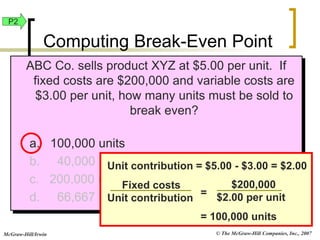
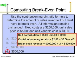
* Unit contribution margin is $5 - $3 = $2
* Contribution margin ratio is $2/$5 = 40%
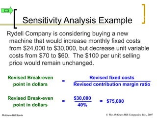
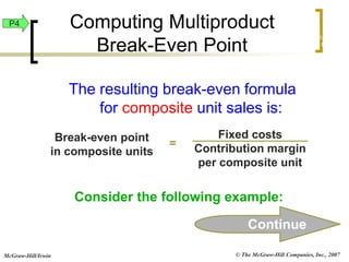
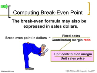
* Break-even point in sales dollars = Fixed costs / Contribution margin ratio
* = $200,000 / 40%
* = $200,000 / 0.4
* = $500,000
Therefore, the amount of sales revenue ABC must have to break even is $500,000.
P2
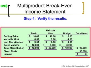
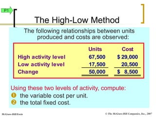
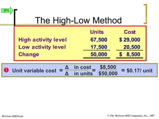
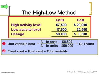
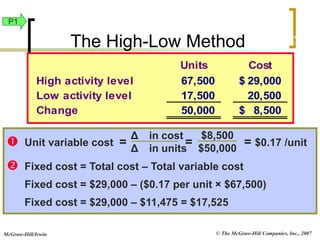
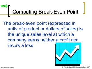
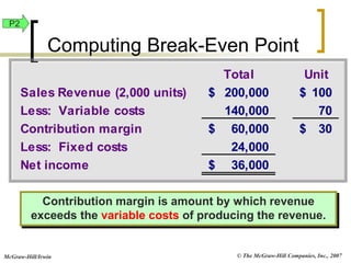
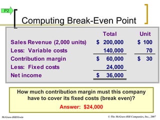
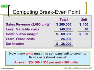
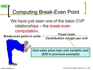
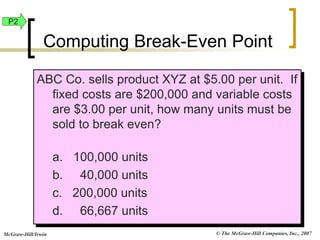
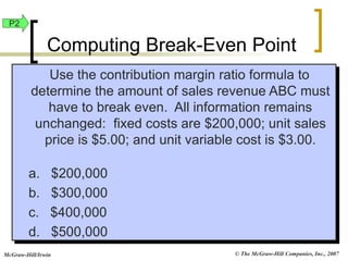
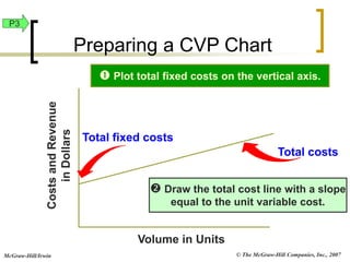
Computing Break-Even Point
�© The McGraw-Hill Companies, Inc., 2007
McGraw-Hill/Irwin
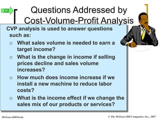
Break-even analysis is useful for:
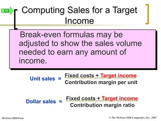
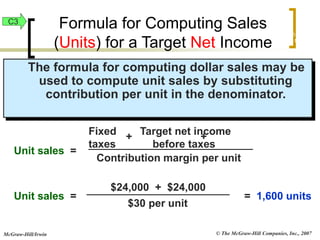
- Determining the sales volume needed to earn a target profit
![© The McGraw-Hill Companies, Inc., 2007
McGraw-Hill/Irwin
Rydell expects to sell 1,500 units at $100
each next month. Fixed costs are $24,000
per month and the unit variable cost is
$70. What amount of income should
Rydell expect?
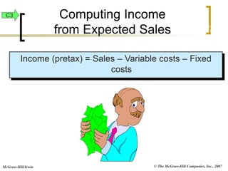
Income (pretax) = Sales – Variable costs – Fixed costs
= [1,500 units × $100] – [1,500 units × $70] – $24,000
= $21,000
Computing Income
from Expected Sales
Exh.
22-13
C3](https://image.slidesharecdn.com/mach05-230321094348-12390ca2/85/yrtyt-41-320.jpg)