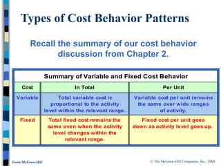
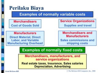
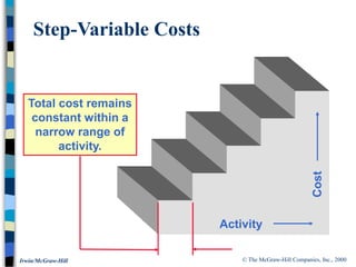
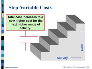
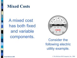
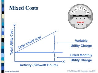
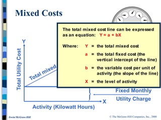
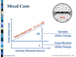
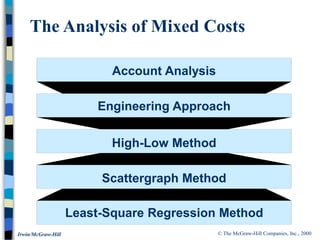
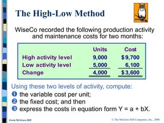
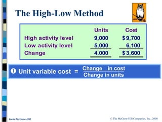
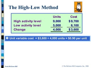
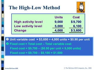
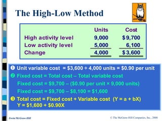
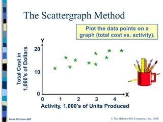
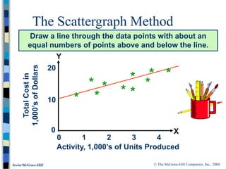
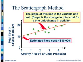
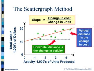
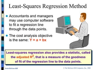
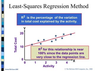
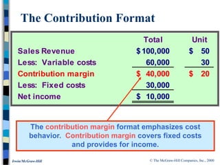
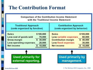
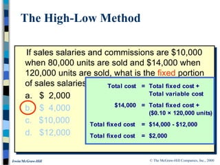
PERILAKU BIAYA :
Analisis dan Penggunaan
BAB
3
© The McGraw-Hill Companies, Inc., 2000
Irwin/McGraw-Hill
Types of Cost Behavior Patterns
Summary of Variable and Fixed Cost Behavior
Cost In Total Per Unit
Variable Total variable cost is Variable cost per unit remains
proportional to the activity the same over wide ranges
level within the relevant range. of activity.
Fixed Total fixed cost remains the Fixed cost per unit goes
same even when the activity down as activity level goes up.
level changes within the
relevant range.
Recall the summary of our cost behavior
discussion from Chapter 2.
© The McGraw-Hill Companies, Inc., 2000
Irwin/McGraw-Hill
Perilaku Biaya
Merchandisers
Cost of Goods Sold
Manufacturers
Direct Material, Direct
Labor, and Variable
Manufacturing Overhead
Merchandisers and
Manufacturers
Sales commissions and
shipping costs
Service Organizations
Supplies and travel
Examples of normally variable costs
Examples of normally fixed costs
Merchandisers, manufacturers, and
service organizations
Real estate taxes, Insurance, Sales salaries
Depreciation, Advertising
© The McGraw-Hill Companies, Inc., 2000
Irwin/McGraw-Hill
The Activity Base
Machine
hours
Labor
hours
Units
produced
Miles
driven
A measure of the event
causing the incurrence of a
variable cost – a cost driver
© The McGraw-Hill Companies, Inc., 2000
Irwin/McGraw-Hill
Step-Variable Costs
Activity
Cost
Total cost remains
constant within a
narrow range of
activity.
© The McGraw-Hill Companies, Inc., 2000
Irwin/McGraw-Hill
Step-Variable Costs
Activity
Cost
Total cost increases to a
new higher cost for the
next higher range of
activity.
© The McGraw-Hill Companies, Inc., 2000
Irwin/McGraw-Hill
The Linearity Assumption and the
Relevant Range
Activity
Total
Cost
Economist’s
Curvilinear Cost
Function
© The McGraw-Hill Companies, Inc., 2000
Irwin/McGraw-Hill
Activity
Total
Cost
Economist’s
Curvilinear Cost
Function
Accountant’s Straight-Line
Approximation (constant
unit variable cost)
The Linearity Assumption and the
Relevant Range
© The McGraw-Hill Companies, Inc., 2000
Irwin/McGraw-Hill
Activity
Total
Cost
Relevant
Range
The Linearity Assumption and the
Relevant Range
Accountant’s Straight-Line
Approximation (constant
unit variable cost)
Economist’s
Curvilinear Cost
Function
A straight line
closely
approximates
a curvilinear
variable cost
line within the
relevant
range.
© The McGraw-Hill Companies, Inc., 2000
Irwin/McGraw-Hill
Types of Fixed Costs
Fixed Costs
Discretionary
May be altered in the
short-term by current
managerial decisions
Committed
Long-term, cannot be
reduced in the short
term.
Examples
Depreciation on
Buildings and
Equipment
Examples
Advertising and
Research and
Development
© The McGraw-Hill Companies, Inc., 2000
Irwin/McGraw-Hill
Trend Toward Fixed Costs
Increased automation.
Increase in salaried knowledge workers
who are difficult to train and replace.
Implications
Managers are more “locked-in” with fewer decision
alternatives.
Planning becomes more crucial because fixed costs are
difficult to change with current operating decisions.
© The McGraw-Hill Companies, Inc., 2000
Irwin/McGraw-Hill
Example: Office space
is available at a rental
rate of $30,000 per
year in increments of
1,000 square feet. As
the business grows
more space is rented,
increasing the total
cost.
Fixed Costs and Relevant Range
Continue
© The McGraw-Hill Companies, Inc., 2000
Irwin/McGraw-Hill
Rent
Cost
in
Thousands
of
Dollars
0 1,000 2,000 3,000
Rented Area (Square Feet)
0
30
60
Fixed Costs and Relevant Range
90
Relevant
Range
Total cost doesn’t
change for a wide
range of activity,
and then jumps to a
new higher cost for
the next higher
range of activity.
© The McGraw-Hill Companies, Inc., 2000
Irwin/McGraw-Hill
How does this type
of fixed cost differ
from a step-variable
cost?
Step-variable costs
can be adjusted more
quickly and . . .
The width of the
activity steps is much
wider for the fixed
cost.
Fixed Costs and Relevant Range
© The McGraw-Hill Companies, Inc., 2000
Irwin/McGraw-Hill
A mixed cost
has both fixed
and variable
components.
Mixed Costs
Consider the
following electric
utility example.
© The McGraw-Hill Companies, Inc., 2000
Irwin/McGraw-Hill
Fixed Monthly
Utility Charge
Variable
Utility Charge
Activity (Kilowatt Hours)
Total
Utility
Cost
Mixed Costs
X
Y
© The McGraw-Hill Companies, Inc., 2000
Irwin/McGraw-Hill
Fixed Monthly
Utility Charge
Variable
Utility Charge
Activity (Kilowatt Hours)
Total
Utility
Cost
Mixed Costs
X
Y
The total mixed cost line can be expressed
as an equation: Y = a + bX
Where: Y = the total mixed cost
a = the total fixed cost (the
vertical intercept of the line)
b = the variable cost per unit of
activity (the slope of the line)
X = the level of activity
© The McGraw-Hill Companies, Inc., 2000
Irwin/McGraw-Hill
Fixed Monthly
Utility Charge
Variable
Utility Charge
Activity (Kilowatt Hours)
Total
Utility
Cost
Mixed Costs
bX
a
X
Y
© The McGraw-Hill Companies, Inc., 2000
Irwin/McGraw-Hill
The Analysis of Mixed Costs
Engineering Approach
Account Analysis
Scattergraph Method
Least-Square Regression Method
High-Low Method
© The McGraw-Hill Companies, Inc., 2000
Irwin/McGraw-Hill
Account Analysis
Each account is classified as either
variable or fixed based on the analyst’s
knowledge of how the account behaves.
© The McGraw-Hill Companies, Inc., 2000
Irwin/McGraw-Hill
Engineering Estimates
Cost estimates are based on an evaluation
of production methods, and material, labor
and overhead requirements.
© The McGraw-Hill Companies, Inc., 2000
Irwin/McGraw-Hill
WiseCo recorded the following production activity
and maintenance costs for two months:
Using these two levels of activity, compute:
 the variable cost per unit;
 the fixed cost; and then
 express the costs in equation form Y = a + bX.
The High-Low Method
Units Cost
High activity level 9,000 9,700
$
Low activity level 5,000 6,100
Change 4,000 3,600
$
© The McGraw-Hill Companies, Inc., 2000
Irwin/McGraw-Hill
 Unit variable cost =
Change in cost
Change in units
Units Cost
High activity level 9,000 9,700
$
Low activity level 5,000 6,100
Change 4,000 3,600
$
The High-Low Method
© The McGraw-Hill Companies, Inc., 2000
Irwin/McGraw-Hill
Units Cost
High activity level 9,000 9,700
$
Low activity level 5,000 6,100
Change 4,000 3,600
$
The High-Low Method
 Unit variable cost = $3,600 ÷ 4,000 units = $0.90 per unit
© The McGraw-Hill Companies, Inc., 2000
Irwin/McGraw-Hill
Units Cost
High activity level 9,000 9,700
$
Low activity level 5,000 6,100
Change 4,000 3,600
$
The High-Low Method
 Unit variable cost = $3,600 ÷ 4,000 units = $0.90 per unit
 Fixed cost = Total cost – Total variable cost
Fixed cost = $9,700 – ($0.90 per unit × 9,000 units)
Fixed cost = $9,700 – $8,100 = $1,600
© The McGraw-Hill Companies, Inc., 2000
Irwin/McGraw-Hill
 Unit variable cost = $3,600 ÷ 4,000 units = $0.90 per unit
 Fixed cost = Total cost – Total variable cost
Fixed cost = $9,700 – ($0.90 per unit × 9,000 units)
Fixed cost = $9,700 – $8,100 = $1,600
 Total cost = Fixed cost + Variable cost (Y = a + bX)
Y = $1,600 + $0.90X
Units Cost
High activity level 9,000 9,700
$
Low activity level 5,000 6,100
Change 4,000 3,600
$
The High-Low Method
© The McGraw-Hill Companies, Inc., 2000
Irwin/McGraw-Hill
The Scattergraph Method
Plot the data points on a
graph (total cost vs. activity).
0 1 2 3 4
*
Total
Cost
in
1,000’s
of
Dollars
10
20
0
*
*
*
*
*
*
*
*
*
Activity, 1,000’s of Units Produced
X
Y
© The McGraw-Hill Companies, Inc., 2000
Irwin/McGraw-Hill
The Scattergraph Method
Draw a line through the data points with about an
equal numbers of points above and below the line.
0 1 2 3 4
*
Total
Cost
in
1,000’s
of
Dollars
10
20
0
*
*
*
*
*
*
*
*
*
Activity, 1,000’s of Units Produced
X
Y
© The McGraw-Hill Companies, Inc., 2000
Irwin/McGraw-Hill
The Scattergraph Method
Estimated fixed cost = $10,000
0 1 2 3 4
*
Total
Cost
in
1,000’s
of
Dollars
10
20
0
*
*
*
*
*
*
*
*
*
Activity, 1,000’s of Units Produced
X
Y
The slope of this line is the variable unit
cost. (Slope is the change in total cost for
a one unit change in activity).
© The McGraw-Hill Companies, Inc., 2000
Irwin/McGraw-Hill
The Scattergraph Method
Slope =
Change in cost
Change in units
Horizontal distance is
the change in activity.
0 1 2 3 4
*
Total
Cost
in
1,000’s
of
Dollars
10
20
0
*
*
*
*
*
*
*
*
*
Activity, 1,000’s of Units Produced
X
Y
Vertical
distance
is the
change
in cost.
© The McGraw-Hill Companies, Inc., 2000
Irwin/McGraw-Hill
 Accountants and managers
may use computer software
to fit a regression line
through the data points.
 The cost analysis objective
is the same: Y = a + bx
Least-Squares Regression Method
Least-squares regression also provides a statistic, called
the adjusted R2, that is a measure of the goodness
of fit of the regression line to the data points.
© The McGraw-Hill Companies, Inc., 2000
Irwin/McGraw-Hill
0 1 2 3 4
Total
Cost
10
20
0
Activity
*
*
*
*
*
*
*
*
*
*
Least-Squares Regression Method
R2 is the percentage of the variation
in total cost explained by the activity.
R2 for this relationship is near
100% since the data points are
very close to the regression line.
X
Y
© The McGraw-Hill Companies, Inc., 2000
Irwin/McGraw-Hill
Let’s put our
knowledge of cost
behavior to work by
preparing a
contribution format
income statement.
The Contribution Format
© The McGraw-Hill Companies, Inc., 2000
Irwin/McGraw-Hill
The Contribution Format
Total Unit
Sales Revenue 100,000
$ 50
$
Less: Variable costs 60,000 30
Contribution margin 40,000
$ 20
$
Less: Fixed costs 30,000
Net income 10,000
$
The contribution margin format emphasizes cost
behavior. Contribution margin covers fixed costs
and provides for income.
© The McGraw-Hill Companies, Inc., 2000
Irwin/McGraw-Hill
The Contribution Format
Used primarily for
external reporting.
Used primarily by
management.
© The McGraw-Hill Companies, Inc., 2000
Irwin/McGraw-Hill
End of Chapter 5
© The McGraw-Hill Companies, Inc., 2000
Irwin/McGraw-Hill
Terimakasih,
see you again,
byeeee….!!!!!!
© The McGraw-Hill Companies, Inc., 2000
Irwin/McGraw-Hill
CONTOH KASUS
© The McGraw-Hill Companies, Inc., 2000
Irwin/McGraw-Hill
If sales salaries and commissions are $10,000
when 80,000 units are sold and $14,000 when
120,000 units are sold, what is the variable
portion of sales salaries and commission?
a. $0.08 per unit
b. $0.10 per unit
c. $0.12 per unit
d. $0.125 per unit
The High-Low Method
© The McGraw-Hill Companies, Inc., 2000
Irwin/McGraw-Hill
If sales salaries and commissions are $10,000
when 80,000 units are sold and $14,000 when
120,000 units are sold, what is the variable
portion of sales salaries and commission?
a. $0.08 per unit
b. $0.10 per unit
c. $0.12 per unit
d. $0.125 per unit
The High-Low Method
$4,000 ÷ 40,000 units
= $0.10 per unit
Units Cost
High level 120,000 14,000
$
Low level 80,000 10,000
Change 40,000 4,000
$
© The McGraw-Hill Companies, Inc., 2000
Irwin/McGraw-Hill
If sales salaries and commissions are $10,000
when 80,000 units are sold and $14,000 when
120,000 units are sold, what is the fixed portion
of sales salaries and commissions?
a. $ 2,000
b. $ 4,000
c. $10,000
d. $12,000
The High-Low Method
© The McGraw-Hill Companies, Inc., 2000
Irwin/McGraw-Hill
If sales salaries and commissions are $10,000
when 80,000 units are sold and $14,000 when
120,000 units are sold, what is the fixed portion
of sales salaries and commissions?
a. $ 2,000
b. $ 4,000
c. $10,000
d. $12,000
The High-Low Method
Total cost = Total fixed cost +
Total variable cost
$14,000 = Total fixed cost +
($0.10 × 120,000 units)
Total fixed cost = $14,000 - $12,000
Total fixed cost = $2,000

b3_perilaku_biaya.ppt

  • 1.
    PERILAKU BIAYA : Analisisdan Penggunaan BAB 3
  • 2.
    © The McGraw-HillCompanies, Inc., 2000 Irwin/McGraw-Hill Types of Cost Behavior Patterns Summary of Variable and Fixed Cost Behavior Cost In Total Per Unit Variable Total variable cost is Variable cost per unit remains proportional to the activity the same over wide ranges level within the relevant range. of activity. Fixed Total fixed cost remains the Fixed cost per unit goes same even when the activity down as activity level goes up. level changes within the relevant range. Recall the summary of our cost behavior discussion from Chapter 2.
  • 3.
    © The McGraw-HillCompanies, Inc., 2000 Irwin/McGraw-Hill Perilaku Biaya Merchandisers Cost of Goods Sold Manufacturers Direct Material, Direct Labor, and Variable Manufacturing Overhead Merchandisers and Manufacturers Sales commissions and shipping costs Service Organizations Supplies and travel Examples of normally variable costs Examples of normally fixed costs Merchandisers, manufacturers, and service organizations Real estate taxes, Insurance, Sales salaries Depreciation, Advertising
  • 4.
    © The McGraw-HillCompanies, Inc., 2000 Irwin/McGraw-Hill The Activity Base Machine hours Labor hours Units produced Miles driven A measure of the event causing the incurrence of a variable cost – a cost driver
  • 5.
    © The McGraw-HillCompanies, Inc., 2000 Irwin/McGraw-Hill Step-Variable Costs Activity Cost Total cost remains constant within a narrow range of activity.
  • 6.
    © The McGraw-HillCompanies, Inc., 2000 Irwin/McGraw-Hill Step-Variable Costs Activity Cost Total cost increases to a new higher cost for the next higher range of activity.
  • 7.
    © The McGraw-HillCompanies, Inc., 2000 Irwin/McGraw-Hill The Linearity Assumption and the Relevant Range Activity Total Cost Economist’s Curvilinear Cost Function
  • 8.
    © The McGraw-HillCompanies, Inc., 2000 Irwin/McGraw-Hill Activity Total Cost Economist’s Curvilinear Cost Function Accountant’s Straight-Line Approximation (constant unit variable cost) The Linearity Assumption and the Relevant Range
  • 9.
    © The McGraw-HillCompanies, Inc., 2000 Irwin/McGraw-Hill Activity Total Cost Relevant Range The Linearity Assumption and the Relevant Range Accountant’s Straight-Line Approximation (constant unit variable cost) Economist’s Curvilinear Cost Function A straight line closely approximates a curvilinear variable cost line within the relevant range.
  • 10.
    © The McGraw-HillCompanies, Inc., 2000 Irwin/McGraw-Hill Types of Fixed Costs Fixed Costs Discretionary May be altered in the short-term by current managerial decisions Committed Long-term, cannot be reduced in the short term. Examples Depreciation on Buildings and Equipment Examples Advertising and Research and Development
  • 11.
    © The McGraw-HillCompanies, Inc., 2000 Irwin/McGraw-Hill Trend Toward Fixed Costs Increased automation. Increase in salaried knowledge workers who are difficult to train and replace. Implications Managers are more “locked-in” with fewer decision alternatives. Planning becomes more crucial because fixed costs are difficult to change with current operating decisions.
  • 12.
    © The McGraw-HillCompanies, Inc., 2000 Irwin/McGraw-Hill Example: Office space is available at a rental rate of $30,000 per year in increments of 1,000 square feet. As the business grows more space is rented, increasing the total cost. Fixed Costs and Relevant Range Continue
  • 13.
    © The McGraw-HillCompanies, Inc., 2000 Irwin/McGraw-Hill Rent Cost in Thousands of Dollars 0 1,000 2,000 3,000 Rented Area (Square Feet) 0 30 60 Fixed Costs and Relevant Range 90 Relevant Range Total cost doesn’t change for a wide range of activity, and then jumps to a new higher cost for the next higher range of activity.
  • 14.
    © The McGraw-HillCompanies, Inc., 2000 Irwin/McGraw-Hill How does this type of fixed cost differ from a step-variable cost? Step-variable costs can be adjusted more quickly and . . . The width of the activity steps is much wider for the fixed cost. Fixed Costs and Relevant Range
  • 15.
    © The McGraw-HillCompanies, Inc., 2000 Irwin/McGraw-Hill A mixed cost has both fixed and variable components. Mixed Costs Consider the following electric utility example.
  • 16.
    © The McGraw-HillCompanies, Inc., 2000 Irwin/McGraw-Hill Fixed Monthly Utility Charge Variable Utility Charge Activity (Kilowatt Hours) Total Utility Cost Mixed Costs X Y
  • 17.
    © The McGraw-HillCompanies, Inc., 2000 Irwin/McGraw-Hill Fixed Monthly Utility Charge Variable Utility Charge Activity (Kilowatt Hours) Total Utility Cost Mixed Costs X Y The total mixed cost line can be expressed as an equation: Y = a + bX Where: Y = the total mixed cost a = the total fixed cost (the vertical intercept of the line) b = the variable cost per unit of activity (the slope of the line) X = the level of activity
  • 18.
    © The McGraw-HillCompanies, Inc., 2000 Irwin/McGraw-Hill Fixed Monthly Utility Charge Variable Utility Charge Activity (Kilowatt Hours) Total Utility Cost Mixed Costs bX a X Y
  • 19.
    © The McGraw-HillCompanies, Inc., 2000 Irwin/McGraw-Hill The Analysis of Mixed Costs Engineering Approach Account Analysis Scattergraph Method Least-Square Regression Method High-Low Method
  • 20.
    © The McGraw-HillCompanies, Inc., 2000 Irwin/McGraw-Hill Account Analysis Each account is classified as either variable or fixed based on the analyst’s knowledge of how the account behaves.
  • 21.
    © The McGraw-HillCompanies, Inc., 2000 Irwin/McGraw-Hill Engineering Estimates Cost estimates are based on an evaluation of production methods, and material, labor and overhead requirements.
  • 22.
    © The McGraw-HillCompanies, Inc., 2000 Irwin/McGraw-Hill WiseCo recorded the following production activity and maintenance costs for two months: Using these two levels of activity, compute:  the variable cost per unit;  the fixed cost; and then  express the costs in equation form Y = a + bX. The High-Low Method Units Cost High activity level 9,000 9,700 $ Low activity level 5,000 6,100 Change 4,000 3,600 $
  • 23.
    © The McGraw-HillCompanies, Inc., 2000 Irwin/McGraw-Hill  Unit variable cost = Change in cost Change in units Units Cost High activity level 9,000 9,700 $ Low activity level 5,000 6,100 Change 4,000 3,600 $ The High-Low Method
  • 24.
    © The McGraw-HillCompanies, Inc., 2000 Irwin/McGraw-Hill Units Cost High activity level 9,000 9,700 $ Low activity level 5,000 6,100 Change 4,000 3,600 $ The High-Low Method  Unit variable cost = $3,600 ÷ 4,000 units = $0.90 per unit
  • 25.
    © The McGraw-HillCompanies, Inc., 2000 Irwin/McGraw-Hill Units Cost High activity level 9,000 9,700 $ Low activity level 5,000 6,100 Change 4,000 3,600 $ The High-Low Method  Unit variable cost = $3,600 ÷ 4,000 units = $0.90 per unit  Fixed cost = Total cost – Total variable cost Fixed cost = $9,700 – ($0.90 per unit × 9,000 units) Fixed cost = $9,700 – $8,100 = $1,600
  • 26.
    © The McGraw-HillCompanies, Inc., 2000 Irwin/McGraw-Hill  Unit variable cost = $3,600 ÷ 4,000 units = $0.90 per unit  Fixed cost = Total cost – Total variable cost Fixed cost = $9,700 – ($0.90 per unit × 9,000 units) Fixed cost = $9,700 – $8,100 = $1,600  Total cost = Fixed cost + Variable cost (Y = a + bX) Y = $1,600 + $0.90X Units Cost High activity level 9,000 9,700 $ Low activity level 5,000 6,100 Change 4,000 3,600 $ The High-Low Method
  • 27.
    © The McGraw-HillCompanies, Inc., 2000 Irwin/McGraw-Hill The Scattergraph Method Plot the data points on a graph (total cost vs. activity). 0 1 2 3 4 * Total Cost in 1,000’s of Dollars 10 20 0 * * * * * * * * * Activity, 1,000’s of Units Produced X Y
  • 28.
    © The McGraw-HillCompanies, Inc., 2000 Irwin/McGraw-Hill The Scattergraph Method Draw a line through the data points with about an equal numbers of points above and below the line. 0 1 2 3 4 * Total Cost in 1,000’s of Dollars 10 20 0 * * * * * * * * * Activity, 1,000’s of Units Produced X Y
  • 29.
    © The McGraw-HillCompanies, Inc., 2000 Irwin/McGraw-Hill The Scattergraph Method Estimated fixed cost = $10,000 0 1 2 3 4 * Total Cost in 1,000’s of Dollars 10 20 0 * * * * * * * * * Activity, 1,000’s of Units Produced X Y The slope of this line is the variable unit cost. (Slope is the change in total cost for a one unit change in activity).
  • 30.
    © The McGraw-HillCompanies, Inc., 2000 Irwin/McGraw-Hill The Scattergraph Method Slope = Change in cost Change in units Horizontal distance is the change in activity. 0 1 2 3 4 * Total Cost in 1,000’s of Dollars 10 20 0 * * * * * * * * * Activity, 1,000’s of Units Produced X Y Vertical distance is the change in cost.
  • 31.
    © The McGraw-HillCompanies, Inc., 2000 Irwin/McGraw-Hill  Accountants and managers may use computer software to fit a regression line through the data points.  The cost analysis objective is the same: Y = a + bx Least-Squares Regression Method Least-squares regression also provides a statistic, called the adjusted R2, that is a measure of the goodness of fit of the regression line to the data points.
  • 32.
    © The McGraw-HillCompanies, Inc., 2000 Irwin/McGraw-Hill 0 1 2 3 4 Total Cost 10 20 0 Activity * * * * * * * * * * Least-Squares Regression Method R2 is the percentage of the variation in total cost explained by the activity. R2 for this relationship is near 100% since the data points are very close to the regression line. X Y
  • 33.
    © The McGraw-HillCompanies, Inc., 2000 Irwin/McGraw-Hill Let’s put our knowledge of cost behavior to work by preparing a contribution format income statement. The Contribution Format
  • 34.
    © The McGraw-HillCompanies, Inc., 2000 Irwin/McGraw-Hill The Contribution Format Total Unit Sales Revenue 100,000 $ 50 $ Less: Variable costs 60,000 30 Contribution margin 40,000 $ 20 $ Less: Fixed costs 30,000 Net income 10,000 $ The contribution margin format emphasizes cost behavior. Contribution margin covers fixed costs and provides for income.
  • 35.
    © The McGraw-HillCompanies, Inc., 2000 Irwin/McGraw-Hill The Contribution Format Used primarily for external reporting. Used primarily by management.
  • 36.
    © The McGraw-HillCompanies, Inc., 2000 Irwin/McGraw-Hill End of Chapter 5
  • 37.
    © The McGraw-HillCompanies, Inc., 2000 Irwin/McGraw-Hill Terimakasih, see you again, byeeee….!!!!!!
  • 38.
    © The McGraw-HillCompanies, Inc., 2000 Irwin/McGraw-Hill CONTOH KASUS
  • 39.
    © The McGraw-HillCompanies, Inc., 2000 Irwin/McGraw-Hill If sales salaries and commissions are $10,000 when 80,000 units are sold and $14,000 when 120,000 units are sold, what is the variable portion of sales salaries and commission? a. $0.08 per unit b. $0.10 per unit c. $0.12 per unit d. $0.125 per unit The High-Low Method
  • 40.
    © The McGraw-HillCompanies, Inc., 2000 Irwin/McGraw-Hill If sales salaries and commissions are $10,000 when 80,000 units are sold and $14,000 when 120,000 units are sold, what is the variable portion of sales salaries and commission? a. $0.08 per unit b. $0.10 per unit c. $0.12 per unit d. $0.125 per unit The High-Low Method $4,000 ÷ 40,000 units = $0.10 per unit Units Cost High level 120,000 14,000 $ Low level 80,000 10,000 Change 40,000 4,000 $
  • 41.
    © The McGraw-HillCompanies, Inc., 2000 Irwin/McGraw-Hill If sales salaries and commissions are $10,000 when 80,000 units are sold and $14,000 when 120,000 units are sold, what is the fixed portion of sales salaries and commissions? a. $ 2,000 b. $ 4,000 c. $10,000 d. $12,000 The High-Low Method
  • 42.
    © The McGraw-HillCompanies, Inc., 2000 Irwin/McGraw-Hill If sales salaries and commissions are $10,000 when 80,000 units are sold and $14,000 when 120,000 units are sold, what is the fixed portion of sales salaries and commissions? a. $ 2,000 b. $ 4,000 c. $10,000 d. $12,000 The High-Low Method Total cost = Total fixed cost + Total variable cost $14,000 = Total fixed cost + ($0.10 × 120,000 units) Total fixed cost = $14,000 - $12,000 Total fixed cost = $2,000