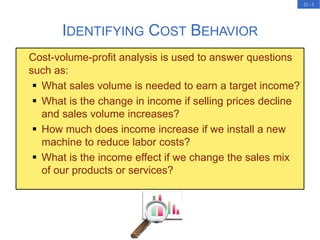
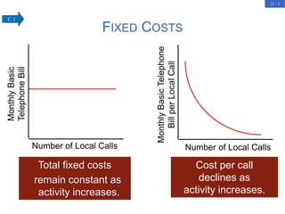
This document provides an overview of cost-volume-profit (CVP) analysis and how it can be used to answer questions about sales volumes, costs, income, and break-even points. It discusses identifying cost behavior as fixed, variable, or mixed; measuring cost behavior using scatter diagrams, the high-low method, and least-squares regression; using break-even analysis to determine the sales volume or dollars needed to cover fixed costs; computing income from sales and costs data; and sensitivity analysis of changes to estimates. Multiproduct CVP analysis and degree of operating leverage are also covered.
Marginal costing is a technique that uses the concept of marginal cost, which is the change in total cost from producing one additional unit. It involves separating total costs into fixed and variable costs. Contribution margin is the difference between selling price and variable cost per unit, and shows the amount available to cover fixed costs and generate profit. Cost-volume-profit (CVP) analysis examines how costs, revenue, and profit change with production volume. It can be used to determine the break-even point and plan production levels required to achieve profit targets. Managers use CVP to make decisions about pricing, production, investment, and financing.
This document discusses key concepts in cost-volume-profit analysis using the example of a bicycle company. It explains the contribution format income statement and how it is used to determine the contribution margin, break-even point, margin of safety, and degree of operating leverage. The contribution margin is the amount of sales revenue left after deducting variable expenses and is used to cover fixed expenses and determine profits. The document provides examples of how profits are affected by changes in sales volume, variable costs, fixed costs, and selling price. It emphasizes the importance of understanding cost behavior and how operating leverage impacts the sensitivity of profits to changes in sales.
1. Calculate contribution margin per customer as average revenue ($8) minus average variable cost ($3), which is $5.
2. Calculate break-even point in customers as fixed costs ($450,000) divided by contribution margin per customer ($5), which is 90,000 customers.
3. Calculate taxable income as contribution margin ($5 per customer) times number of customers minus fixed costs ($450,000).
4. Calculate income taxes as 30% of taxable income.
5. Calculate net income as taxable income minus income taxes.
This document outlines key concepts in cost-volume-profit (CVP) analysis including:
- Variable and fixed costs and how they are affected by changes in activity levels
- Calculating break-even points in units and dollars using contribution margin and equation methods
- Constructing and interpreting CVP graphs
- Determining sales volumes needed to reach target profit levels
- Analyzing the effects of operating leverage and sales mix on profits
Examples are provided to demonstrate calculating break-even points for non-profit organizations and analyzing the impact of changes in sales mix.
This document provides an overview of cost-volume-profit (CVP) analysis, which examines how a firm's sales volume, selling price, cost structure, and profitability interact. It presents the basic one-product CVP model using equations and contribution margin concepts. Key assumptions of the CVP model are discussed. The document also covers break-even analysis, target profit analysis, margin of safety, changes in variables, multi-product CVP models, operating leverage, and an example problem analyzing CVP relationships for a company.
This document discusses cost-volume-profit (CVP) analysis through six learning objectives. It provides examples and formulas to calculate break-even points, target profits, revenue requirements, and the impact of multiple products. Graphs are presented to illustrate profit-volume and cost-volume-profit relationships. The document explains that CVP analysis assumes linear cost and revenue functions and examines how risk, uncertainty, and changing variables affect CVP results. Managers are advised to consider margin of safety, operating leverage, and sensitivity analysis when using CVP analysis under uncertainty.
Contribution is revenue minus variable costs. It represents the amount available to cover fixed costs and generate profit. The contribution margin ratio is contribution divided by sales revenue and expresses what percentage of sales is available for fixed costs and profit. It is calculated by taking the difference between total sales and total variable costs, then dividing by total sales. Higher contribution margin ratios indicate more sales revenue available for covering fixed costs and generating profit.
Risk Analysis and Project Evaluation/Abshor.Marantika/Gita Mutiara Ovelia/3-3gitaovelia
1. Risk analysis is important for project evaluation because project cash flows are risky and may differ from estimates, and forecasts are made by humans who can be optimistic.
2. Sensitivity analysis evaluates the effect of each value driver on NPV and identifies the most impactful variable. Scenario analysis considers simultaneous changes to multiple drivers. Simulation generates thousands of value combinations to model outcomes.
3. Break-even analyses determine the sales or output level needed to cover costs, including accounting, cash, and NPV break-even points.
This document provides an overview of absorption costing and marginal costing. Absorption costing treats all manufacturing costs, including fixed costs, as product costs. Marginal costing treats only variable manufacturing costs as product costs and regards fixed costs as period costs. The document also discusses the treatment of fixed overheads, valuation of closing stock, and reported profit under each method. It then covers the concepts of break-even analysis including calculation of break-even point, target profit, margin of safety, and the impact of changes in cost and revenue components. The limitations of break-even analysis are also summarized.
Marginal costing involves separating variable costs from fixed costs when calculating the cost per unit of production. This allows for better decision making as fixed costs do not change with production volume. Total cost includes fixed costs allocated to each unit and is not suitable for decisions about changes in production volume. Marginal costing shows that the firm should accept an order that reduces the selling price from $12 to $8 per unit as contribution and profit will increase by $400.
Sales mix, or the proportions of different products sold, can impact profits even if total sales remain the same. Introducing a new low-profit product or dropping a high-profit one can decrease profits. Companies can improve profits in a slow-growth market by shifting sales mix toward higher-profit products. Sales managers must consider sales mix when setting commission plans to incentivize selling profitable items. A sales mix variance calculation measures differences between actual and planned sales mixes.
Akuntansi Manajemen Edisi 8 oleh Hansen & Mowen Bab 11Dwi Wahyu
This document discusses cost-volume-profit (CVP) analysis, which expresses the break-even point, impact of changes in fixed costs on profit, and sensitivity of profit to price and cost changes. It provides learning objectives, definitions of key CVP terms, formulas for calculating break-even units and sales, and an example of a multiple product CVP analysis. The document also discusses assumptions of CVP analysis, profit-volume and cost-volume graphs, and the impact of risk, uncertainty and activity-based costing on CVP.
The document discusses operational auditing and concepts related to evaluating organizational effectiveness and efficiency. It defines operational auditing as evaluating the effectiveness and/or efficiency of operations, with effectiveness referring to accomplishing objectives and efficiency meaning reducing costs without reducing effectiveness. Economy is defined as maximizing the use of limited resources to achieve goals. Examples of types of inefficiency include acquiring goods and services too costly, lack of bids for purchases, raw materials not being available when needed, duplication of employee efforts, and work being done that serves no purpose.
This document discusses the key differences between managerial accounting and financial accounting. Managerial accounting provides internal information for managers to use for planning, directing, monitoring and controlling operations, while financial accounting provides external information to stakeholders. It also discusses decision-making tools in managerial accounting like contribution margin and break-even analysis which are used to evaluate product lines and determine the sales volume needed to cover total costs.
This document discusses break-even analysis and cost-volume-profit analysis. It defines break-even analysis as determining the level at which costs and revenues are equal. It explains how to calculate the break-even point by determining fixed and variable expenses. It provides an example of calculating contribution margin ratio and break-even point using sales, fixed expenses, and variable expenses. It also discusses how changes in factors like sales price, expenses, or sales volume impact break-even analysis.
This document discusses break even analysis, including cost-volume-profit (CVP) analysis, contribution, break even point, margin of safety, and break even charts. It defines key terms like contribution, break even point, and margin of safety. The break even point is where total sales equal total variable costs plus fixed costs. Margin of safety is the point above which profit is made. Break even charts graphically show the break even point and relationship between costs, sales, and activity levels. The document also covers multi-product break even analysis and the limitations of CVP analysis.
This document discusses cost-volume-profit (CVP) analysis and its applications in business decision making. It defines fixed and variable costs and explains how CVP analysis explores the relationship between costs, activity levels, and profits. A key aspect of CVP is calculating the break-even point, which is the sales volume where total revenue equals total costs, resulting in zero profit. The document also outlines assumptions of break-even analysis and how to calculate break-even points using equations or graphs. It provides examples of using CVP to determine profit levels at different volumes and to calculate sales needed to achieve a target profit.
unit 2 CVP analysis, Break-even point.pptxuday231983
The National Anti-profiteering Authority (NAA) in India has issued letters to 50 consumer goods companies and over-the-counter drug makers to check if they have passed on the benefits of reduced GST rates to consumers. NAA is questioning the pricing strategies of companies like Mankind Pharma, Johnson & Johnson, and Colgate-Palmolive. Cost-volume-profit (CVP) analysis is an important tool that provides information on the behavior of costs with changes in volume, break-even points, sensitivity of profits to output changes, and profits for projected sales levels. Break-even analysis determines the sales volume needed to cover total costs and is a key aspect of CVP analysis.
This document provides an overview of absorption costing and marginal costing. Absorption costing treats all manufacturing costs, including fixed costs, as product costs. Marginal costing treats only variable manufacturing costs as product costs, regarding fixed costs as period costs. Absorption costing results in higher inventory valuations and can result in different profit amounts than marginal costing depending on production and sales levels. The document also discusses breakeven analysis and how it can be used to determine sales volumes needed to reach the breakeven point or a target profit level.
CVP (cost-volume-profit) analysis examines the relationships between costs, volume, and profit. It is a useful short-term planning tool for decision making. Key elements include break-even point, contribution margin, and profit-volume charts. CVP assumes fixed costs are constant at all activity levels and unit variable costs are also constant. It can be applied to single or multiple products if they have a fixed sales mix. The document provides an example CVP analysis for a company with three hair product lines.
This document discusses different types of costs including fixed costs, variable costs, average costs, and marginal costs. It provides examples of each type of cost and explains how they relate to total cost, average cost, and profit analysis. The key points made include:
- Fixed costs do not depend on output while variable costs do depend on output. Total cost is the sum of fixed and variable costs.
- Average cost is total cost divided by output and depends on the ratio of fixed costs to output. Marginal cost is the change in total cost from a one unit change in output and depends only on variable costs.
- The relationship between average cost, marginal cost, and output determines if a company experiences economies of
This document discusses concepts related to cost-volume-profit analysis and break-even analysis. It defines marginal costing, contribution margin, profit-volume ratio, break-even point, and margin of safety. It also includes examples showing how to calculate these metrics using cost and revenue data. The document is intended to help managers understand how costs, sales volume, and price affect profitability.
Top of Form 1.Award 8.33 pointsPringle Company distribu.docxturveycharlyn
Top of Form
1.
Award: 8.33 points
Pringle Company distributes a single product. The company’s sales and expenses for a recent month follow:
Total
Per Unit
Sales
$
300,000
$
20
Variable expenses
210,000
14
Contribution margin
90,000
$
6
Fixed expenses
78,000
Net operating income
$
12,000
Required:
1.
What is the monthly break-even point in units sold and in sales dollars? (Omit the "$" sign in your response.)
Break-even point in unit sales
units
Break-even point in sales dollars
$
2.
Without resorting to computations, what is the total contribution margin at the break-even point? (Omit the "$" sign in your response.)
Total contribution margin
$
3.
How many units would have to be sold each month to earn a target profit of $31,200? Use the formula method.
Units sold
4.
Refer to the original data. Compute the company's margin of safety in both dollar and percentage terms. (Round your percentage answer to 2 decimal places. Omit the "$" and "%" signs in your response.)
Dollars
Percentage
Margin of safety
$
%
5.
What is the company’s CM ratio? If monthly sales increase by $61,000 and there is no change in fixed expenses, by how much would you expect monthly net operating income to increase? (Omit the "$" and "%" signs in your response.)
CM ratio
%
Net operating income increases by
$
References
WorksheetLearning Objective: 05-03 Use the contribution margin ratio (CM ratio) to compute changes in contribution margin and net operating income resulting from changes in sales volume.Learning Objective: 05-07 Compute the margin of safety and explain its significance.
Difficulty: EasyLearning Objective: 05-05 Determine the level of sales needed to achieve a desired target profit.
Learning Objective: 05-01 Explain how changes in activity affect contribution margin and net operating income.Learning Objective: 05-06 Determine the break-even point.
2.
Award: 8.33 points
Reveen Products sells camping equipment. One of the company’s products, a camp lantern, sells for $130 per unit. Variable expenses are $91 per lantern, and fixed expenses associated with the lantern total $179,400 per month.
Required:
1.
Compute the company’s break-even point in number of lanterns and in total sales dollars. (Omit the "$" sign in your response.)
Number of lanterns
Total sales dollars
$
2.
If the variable expenses per lantern increase as a percentage of the selling price, will it result in a higher or a lower break-even point? (Assume that the fixed expenses remain unchanged.)
Higher break-even point
Lower break-even point
3.
At present, the company is selling 16,000 lanterns per month. The sales manager is convinced that a 10% reduction in the selling price will result in a 25% increase in the number of lanterns sold each month. Prepare two contribution format income statements, one under present operating conditions, a ...
The document discusses cost-volume-profit (CVP) analysis, which examines how sales volume, price, costs, and profitability interact. CVP analysis uses models to help managers make decisions about marketing, production, investment, and financing. The one-product CVP model calculates net income as the difference between total revenue and total costs. It can be used to determine the break-even point and target profits. For companies with multiple products, the CVP model is modified to account for different sales volumes and costs across products. Operating leverage measures how sensitive operating income is to changes in sales volume.
The document discusses cost-volume-profit (CVP) analysis, which studies the effects of output volume on revenue, expenses, and profit. It defines variable and fixed costs, and explains that the break-even point is where sales equal total expenses. Managers use CVP analysis to determine sales volumes needed to reach profit targets or break even. The contribution margin method and equation method for calculating break-even points are also summarized.
This document summarizes absorption costing and marginal costing. Absorption costing treats all manufacturing costs, including both fixed and variable costs, as product costs. Marginal costing treats only variable manufacturing costs as product costs, regarding fixed costs as period costs. Absorption costing follows generally accepted accounting principles but may distort profits, while marginal costing is more relevant for decision making but can manipulate profits. Breakeven analysis uses cost-volume concepts to determine sales needed to cover total costs and achieve a target profit level.
This document provides information about the appraisal process for locum doctors working through NHS Professionals. It discusses the framework, which includes collecting End of Placement Assessment Reports, compiling a portfolio, being matched with an appraiser, conducting the appraisal interview, and completing evaluation forms. It also covers protocols around confidentiality, with exceptions if patient safety issues arise. The overall goal is to support locum doctors' professional development and preparation for revalidation through a standardized appraisal process.
This document provides information about the system requirements and data dictionary for the Hospital Compare Downloadable Database. It describes the various types of measures included in the database, such as general hospital information, patient experience surveys, clinical outcomes, procedure and payment data. For each measure, it outlines the data collection period, reporting cycle, and calculating methodology at a high level. The purpose is to help users navigate and understand the extensive amount of quality data available for thousands of US hospitals.
The document outlines the agenda for day one of a course on budgets and managing money. The day includes sessions on introductions, finance terminology, budgeting fundamentals and basics, parts of a budget, and the budgeting process. There will also be icebreakers, lunch, and energizers. The course overview defines the goals as learning to prepare budgets of any size, getting a budget approved, and making better financial decisions.
The document outlines the HR Plan to Win, which provides a framework to guide strategic HR planning. It discusses the purpose of establishing measurable goals for HR and focusing efforts on critical areas like talent, employment experience, and rewards. Key people metrics are highlighted to monitor progress. The summary focuses on areas of emphasis for 2007, including improving the manager experience, respectful workplace training, leadership development programs, and globalizing rewards and employment branding initiatives.
The document provides an introduction to the global tea industry and discusses some tea trends. It notes that tea has been consumed for ages due to its health benefits. Different teas provide benefits like boosting the immune system and reducing inflammation. Some tea trends mentioned are bubble tea and K-cups.
This document provides an overview of key economic concepts including:
- Economics is the study of how societies allocate scarce resources to satisfy unlimited wants. It can be divided into microeconomics and macroeconomics.
- The economic problem involves determining what, how, and for whom to produce goods and services.
- Opportunity cost, tradeoffs, and rational decision making are important concepts in economics for understanding how individuals and societies make choices.
This document discusses production functions and costs. It defines key concepts such as:
- Production functions show the relationship between inputs and maximum possible output. Short run production is fixed capital while variable inputs can change. Long run all inputs can vary.
- Cost concepts include total, average, and marginal costs. Total cost is the sum of total fixed and variable costs. Marginal cost is the change in total cost from a one unit change in output.
- Cost curves are U-shaped as average and marginal costs initially fall then rise due to diminishing returns. Minimum points indicate optimal output levels for firms.
This document discusses positioning strategies from the textbook "Marketing Management" by Kotler and Keller. It defines positioning as designing a company's offering and image to occupy a distinctive place in the customer's mind. Effective positioning creates a value proposition that gives customers a strong reason to buy a product. The document outlines developing positioning strategies, including determining the target market, identifying relevant competitors, and choosing optimal points of difference and parity. It also discusses using brand mantras to summarize a brand's positioning and differentiate brands through employees, channels, image, and services. Overall positioning strategies aim to communicate a simple and compelling message about a brand's identity and benefits.
This document summarizes key concepts from a marketing management textbook chapter on market segmentation and targeting. It discusses how companies can segment consumer and business markets using geographic, demographic, psychographic, and behavioral factors. The key requirements for effective segmentation are that segments are measurable, substantial, accessible, differentiable, actionable. Companies must then evaluate segments and choose target markets based on objectives, resources, attractiveness, size, and growth. Targeting strategies range from undifferentiated to differentiated to niche to customized marketing.
Marketing research involves a 6-step process: 1) defining the problem, 2) developing a research plan, 3) collecting information, 4) analyzing the information, 5) presenting findings, and 6) making a decision. Good marketing research is objective, relevant, accurate, reliable, timely, and accessible. It follows this process and utilizes various research methods and tools to gather and interpret meaningful data to inform business decisions.
This document summarizes key concepts from the first chapter of the marketing textbook "Marketing Management" by Kotler and Keller. It discusses why marketing is important, defines the scope of marketing, and outlines some core marketing concepts. It also examines how marketing has changed due to new technologies, globalization, and social responsibility. Specifically, it explores how these forces have enhanced capabilities for both consumers and companies. Finally, it identifies the main tasks involved in successful marketing management.
This document discusses standard costs and variances. It begins by defining standards and budgets, and how standards are set for direct materials, direct labor, and manufacturing overhead. It then explains how to calculate variances for direct materials, direct labor, and manufacturing overhead. Specifically, it shows how to calculate total, price, and quantity variances for direct materials, direct labor, and manufacturing overhead. It also discusses potential causes of variances.
Organizational behavior (OB) is defined as the field that studies how individuals and groups act within organizations and how their behaviors impact organizational effectiveness. OB draws from psychology, sociology, anthropology, and other behavioral sciences to understand employee attitudes, behaviors, and performance. The document outlines key OB concepts like how OB can help managers improve productivity and job satisfaction. It also discusses challenges and opportunities for managers to apply OB principles in areas like leadership, communication, and change management.
A review of the growth of the Israel Genealogy Research Association Database Collection for the last 12 months. Our collection is now passed the 3 million mark and still growing. See which archives have contributed the most. See the different types of records we have, and which years have had records added. You can also see what we have for the future.
A workshop hosted by the South African Journal of Science aimed at postgraduate students and early career researchers with little or no experience in writing and publishing journal articles.
The simplified electron and muon model, Oscillating Spacetime: The Foundation...RitikBhardwaj56
Discover the Simplified Electron and Muon Model: A New Wave-Based Approach to Understanding Particles delves into a groundbreaking theory that presents electrons and muons as rotating soliton waves within oscillating spacetime. Geared towards students, researchers, and science buffs, this book breaks down complex ideas into simple explanations. It covers topics such as electron waves, temporal dynamics, and the implications of this model on particle physics. With clear illustrations and easy-to-follow explanations, readers will gain a new outlook on the universe's fundamental nature.
How to Fix the Import Error in the Odoo 17Celine George
An import error occurs when a program fails to import a module or library, disrupting its execution. In languages like Python, this issue arises when the specified module cannot be found or accessed, hindering the program's functionality. Resolving import errors is crucial for maintaining smooth software operation and uninterrupted development processes.
हिंदी वर्णमाला पीपीटी, hindi alphabet PPT presentation, hindi varnamala PPT, Hindi Varnamala pdf, हिंदी स्वर, हिंदी व्यंजन, sikhiye hindi varnmala, dr. mulla adam ali, hindi language and literature, hindi alphabet with drawing, hindi alphabet pdf, hindi varnamala for childrens, hindi language, hindi varnamala practice for kids, https://www.drmullaadamali.com
This presentation includes basic of PCOS their pathology and treatment and also Ayurveda correlation of PCOS and Ayurvedic line of treatment mentioned in classics.
How to Manage Your Lost Opportunities in Odoo 17 CRMCeline George
Odoo 17 CRM allows us to track why we lose sales opportunities with "Lost Reasons." This helps analyze our sales process and identify areas for improvement. Here's how to configure lost reasons in Odoo 17 CRM
How to Add Chatter in the odoo 17 ERP ModuleCeline George
In Odoo, the chatter is like a chat tool that helps you work together on records. You can leave notes and track things, making it easier to talk with your team and partners. Inside chatter, all communication history, activity, and changes will be displayed.
Exploiting Artificial Intelligence for Empowering Researchers and Faculty, In...Dr. Vinod Kumar Kanvaria
Exploiting Artificial Intelligence for Empowering Researchers and Faculty,
International FDP on Fundamentals of Research in Social Sciences
at Integral University, Lucknow, 06.06.2024
By Dr. Vinod Kumar Kanvaria
2. 22 - 2
Cost-volume-profit analysis is used to answer questions
such as:
What sales volume is needed to earn a target income?
What is the change in income if selling prices decline
and sales volume increases?
How much does income increase if we install a new
machine to reduce labor costs?
What is the income effect if we change the sales mix
of our products or services?
IDENTIFYING COST BEHAVIOR
3. 22 - 3
FIXED COSTS
Total fixed costs
remain constant as
activity increases.
Number of Local Calls
Monthly
Basic
Telephone
Bill
Cost per call
declines as
activity increases.
Number of Local Calls
Monthly
Basic
Telephone
Bill
per
Local
Call
C 1
4. 22 - 4
VARIABLE COSTS
Total variable costs
increase as
activity increases.
Minutes Talked
Total
Costs
Cost
per
Minute
Minutes Talked
Cost per Minute
is constant as
activity increases.
C 1
5. 22 - 5
MIXED COSTS
Mixed costs contain a fixed portion that is incurred even when
the facility is unused, and a variable portion that increases with
usage. Utilities typically behave in this manner.
Fixed Monthly
Utility Charge
Variable
Cost per KW
Activity (Kilowatt Hours)
Total
Utility
Cost
C 1
6. 22 - 6
STEP-WISE COSTS
Total cost increases to a new higher cost for the next
higher range of activity, but remains constant within a
range of activity.
C 1
7. 22 - 7
CURVILINEAR COSTS
Costs that increase when activity
increases, but in a nonlinear manner.
C 1
8. 22 - 8
MEASURING COST BEHAVIOR
The objective is to classify all costs as either fixed
or variable. We will look at three methods:
1. Scatter diagrams.
2. The high-low method.
3. Least–squares regression.
A scatter diagram is a plot of cost data points on a
graph. It is almost always helpful to plot cost data to
be able to observe a visual picture of the relationship
between cost and activity.
P 1
9. 22 - 9
0 1 2 3 4 5 6
*
Total
Cost
in
1,000’s
of
Dollars
10
20
0
*
*
*
*
*
*
*
*
*
Activity, 1,000’s of Units Produced
Estimated fixed cost = 10,000
Draw a line through the plotted data points so that about
equal numbers of points fall above and below the line.
SCATTER DIAGRAMS
P 1
10. 22 - 10
Vertical
distance
is the
change
in cost.
Horizontal distance is
the change in activity.
Unit Variable Cost = Slope =
Δ in cost
Δ in units
0 1 2 3 4 5 6
*
Total
Cost
in
1,000’s
of
Dollars
10
20
0
*
*
*
*
*
*
*
*
*
Activity, 1,000’s of Units Produced
SCATTER DIAGRAMS
P 1
11. 22 - 11
The following relationships between units
produced and total cost are observed:
Using these two levels of activity, compute:
the variable cost per unit.
the total fixed cost.
THE HIGH-LOW METHOD
P 1
12. 22 - 12
Units Cost
High activity level - December 67,500 29,000
$
Low activity level - January 17,500 20,500
Change in activity 50,000 8,500
$
Variable cost per unit is determined as follows:
Fixed costs are determined as follows:
THE HIGH-LOW METHOD
Total cost = $17,525 + $0.17 per unit produced
P 1
13. 22 - 13
The objective of the cost
analysis remains the
same: determination of
total fixed cost and the
variable unit cost.
LEAST-SQUARES REGRESSION
Least-squares regression is usually covered
in advanced cost accounting courses. It is
commonly used with spreadsheet programs
or calculators.
P 1
14. 22 - 14
USING BREAK-EVEN ANALYSIS
The break-even point (expressed in
units of product or dollars of sales) is the
unique sales level at which a company
earns neither a profit nor incurs a loss.
A 1
15. 22 - 15
Contribution margin is the amount by which revenue
exceeds the variable costs of producing the revenue.
CONTRIBUTION MARGIN AND ITS
MEASURES
Total contribution margin is $60,000 and the
contribution margin per unit sold is $30.
Total Unit
Sales Revenue (2,000 units) 200,000
$ 100
$
Less: Variable costs 140,000 70
Contribution margin 60,000
$ 30
$
Less: Fixed costs 24,000
Net income 36,000
$
A 1
16. 22 - 16
CONTRIBUTION MARGIN AND ITS
MEASURES
Total Unit
Sales Revenue (2,000 units) 200,000
$ 100
$
Less: Variable costs 140,000 70
Contribution margin 60,000
$ 30
$
Less: Fixed costs 24,000
Net income 36,000
$
Contribution
margin ratio
Contribution margin per unit
Sales price per unit
=
Contribution
margin ratio
=
$30 per unit
$100 per unit
= 30%
A 1
17. 22 - 17
How much contribution margin must Rydell Company
have to cover its fixed costs (break-even)?
Answer: $24,000
Total Unit
Sales Revenue (2,000 units) 200,000
$ 100
$
Less: Variable costs 140,000 70
Contribution margin 60,000
$ 30
$
Less: Fixed costs 24,000
Net income 36,000
$
COMPUTING THE BREAK-EVEN POINT
How many units must Rydell sell to cover its fixed
costs (break-even)?
Answer: $24,000 ÷ $30 per unit = 800 units
P 2
18. 22 - 18
Unit sales price less unit variable cost
($30 in previous example)
We have just seen one of the basic CVP
relationships – the break-even computation.
COMPUTING THE BREAK-EVEN POINT
Break-even point in units =
Fixed costs
Contribution margin per unit
P 2
19. 22 - 19
The break-even formula may also be
expressed in sales dollars.
COMPUTING THE BREAK-EVEN POINT
Unit contribution margin
Unit sales price
Break-even point in dollars =
Fixed costs
Contribution margin ratio
P 2
21. 22 - 21
A limited range of activity called the relevant
range, where CVP relationships are linear.
Unit selling price remains constant.
Unit variable costs remain constant.
Total fixed costs remain constant.
Production = sales (no inventory changes).
MAKING ASSUMPTIONS IN
COST-VOLUME-PROFIT ANALYSIS
P 3
22. 22 - 22
WORKING WITH CHANGES
IN ESTIMATES
What happens to the break-even point if management can
increase the sales price to $105, with no changes in fixed or
variable costs?
Break-even point in units =
Fixed costs
Contribution margin per unit
Break-even point in units =
$24,000
$105 – $70
= 686 units
Total Unit
Sales Revenue (2,000 units) 200,000
$ 100
$
Less: Variable costs 140,000 70
Contribution margin 60,000
$ 30
$
Less: Fixed costs 24,000
Net income 36,000
$
P 3
23. 22 - 23
Income (pretax) = Sales – Variable costs – Fixed costs
COMPUTING INCOME
FROM SALES AND COSTS
Rydell expects to sell 1,500 units at $100 each next month.
Fixed costs are $24,000 per month and the unit variable
cost is $70. What amount of income should Rydell expect?
Income (pretax) = Sales – Variable costs – Fixed costs
= [1,500 units × $100] – [1,500 units × $70] – $24,000
= $21,000
C 2
24. 22 - 24
COMPUTING SALES
FOR A TARGET INCOME
Break-even formulas may be adjusted to show the
sales volume needed to earn any amount of income.
Unit sales =
Fixed costs + Target pretax income
Contribution margin per unit
Dollar sales =
Fixed costs + Target pretax income
Contribution margin ratio
C 2
25. 22 - 25
Before-tax income =
Target net income
1 - tax rate
COMPUTING SALES (DOLLARS) FOR A
TARGET NET INCOME
To convert target net income to before-tax
income, use the following formula:
C 2
26. 22 - 26
COMPUTING SALES (DOLLARS) FOR A
TARGET NET INCOME
Rydell has a monthly target net income of $9,000. The
unit selling price is $100. Monthly fixed costs are
$24,000, the unit variable cost is $70, and the tax rate is
25 percent.
What is Rydell’s target pretax income?
Pretax income =
Target net income
1 - tax rate
Pretax income = = $12,000
$9,000
1 - .25
C 2
27. 22 - 27
COMPUTING SALES (DOLLARS) FOR A
TARGET NET INCOME
Rydell has a monthly target after-tax income of $9,000.
The unit selling price is $100. Monthly fixed costs are
$24,000, the unit variable cost is $70, and the tax rate is
25 percent. Let’s compute the sales revenue that Rydell
will need to earn $12,000 of pretax income?
Dollar sales =
Fixed costs + Target pretax income
Contribution margin ratio
Dollar sales = = $120,000
$24,000 + $12,000
30%
C 2
28. 22 - 28
Contribution margin per unit
Unit sales =
Fixed costs + Target pretax income
Unit sales = = 1,200 units
$24,000 + $12,000
$30 per unit
COMPUTING SALES (UNITS) FOR A
TARGET NET INCOME
The formula for computing dollar sales may be
used to compute unit sales by substituting
contribution per unit in the denominator.
C 2
29. 22 - 29
COMPUTING THE MARGIN OF SAFETY
Margin of safety is the amount by which sales can drop
before the company incurs a loss. Margin of safety may
be expressed as a percentage of expected sales.
Margin of safety Expected sales - Break-even sales
percentage Expected sales
=
If Rydell’s sales are $100,000 and break-even sales are
$80,000, what is the margin of safety percentage?
C 2
Margin of safety $100,000 - $80,000
percentage $100,000
= = 20%
30. 22 - 30
Rydell Company is considering buying a new machine
that would increase monthly fixed costs from $24,000 to
$30,000, but decrease unit variable costs from $70 to $60.
The $100 per unit selling price would remain unchanged.
What is the new break-even point in dollars?
USING SENSITIVITY ANALYSIS
Revised Break-even
point in dollars
Revised fixed costs
Revised contribution margin ratio
Revised Break-even
point in dollars
$30,000
40%
= $75,000
=
=
C 2
31. 22 - 31
The CVP formulas can be modified for use when a
company sells more than one product.
The unit contribution margin is replaced with the
contribution margin for a composite unit.
A composite unit is composed of specific numbers of
each product in proportion to the product sales mix.
Sales mix is the ratio of the volumes of the various
products.
COMPUTING A MULTIPRODUCT
BREAK-EVEN POINT
P 4
32. 22 - 32
The resulting break-even formula
for composite unit sales is:
Break-even point
in composite units
Fixed costs
Contribution margin
per composite unit
=
Consider the following example:
Continue
COMPUTING A MULTIPRODUCT
BREAK-EVEN POINT
P 4
34. 22 - 34
Haircuts
Basic Ultra Budget
Selling Price 20.00
$ 32.00
$ 16.00
$
Variable Cost 13.00 18.00 8.00
Unit Contribution 7.00
$ 14.00
$ 8.00
$
Sales Mix Ratio 4 2 1
Hair-Today offers three cuts as shown below. Annual fixed
costs are $192,000. Compute the break-even point in
composite units and in number of units for each haircut at the
given sales mix.
A 4:2:1 sales mix means that if there are 500 budget cuts,
then there will be 1,000 ultra cuts, and 2,000 basic cuts.
COMPUTING A MULTIPRODUCT
BREAK-EVEN POINT
P 4
35. 22 - 35
Haircuts
Basic Ultra Budget
Selling Price $20.00 $32.00 $16.00
Variable Cost 13.00 18.00 8.00
Unit Contribution $7.00 $14.00 $8.00
Sales Mix Ratio × 4 × 2 × 1
Weighted Contribution 28.00
$ + 28.00
$ + 8.00
$ = 64.00
$
Contribution margin per composite unit
Step 1: Compute contribution margin per
composite unit.
COMPUTING A MULTIPRODUCT
BREAK-EVEN POINT
P 4
36. 22 - 36
Break-even point
in composite units
Fixed costs
Contribution margin
per composite unit
=
Step 2: Compute break-even point in
composite units.
Break-even point
in composite units
$192,000
$64.00 per
composite unit
=
Break-even point
in composite units
= 3,000 composite units
COMPUTING A MULTIPRODUCT
BREAK-EVEN POINT
P 4
37. 22 - 37
Sales Composite
Product Mix Cuts Haircuts
Basic 4 × 3,000 = 12,000
Ultra 2 × 3,000 = 6,000
Budget 1 × 3,000 = 3,000
Total 21,000
Step 3: Determine the number of each haircut
that must be sold to break-even.
COMPUTING A MULTIPRODUCT
BREAK-EVEN POINT
P 4
38. 22 - 38
Step 4: Verify the results.
MULTIPRODUCT BREAK-EVEN
INCOME STATEMENT
P 4
39. 22 - 39
GLOBAL VIEW
Over 90 percent of German companies
surveyed report their cost accounting systems
focus on contribution margin. This focus helps
German companies like Volkswagen control
costs and plan their production levels.
40. 22 - 40
A measure of the extent to which fixed costs are
being used in an organization.
A measure of how a percentage change in
sales will affect profits.
Contribution margin
Pretax income
= Degree of operating leverage
DEGREE OF OPERATING LEVERAGE
A 2
41. 22 - 41
Rydell Company
Sales (1,200 units) 120,000
$
Less: variable expenses 84,000
Contribution margin 36,000
Less: fixed expenses 24,000
Pretax income 12,000
$
$36,000
$12,000
= 3.0
Contribution margin
Net income
= Degree of operating leverage =
If Rydell increases sales by 10 percent, what will the
percentage increase in income be?
OPERATING LEVERAGE
Percent increase in sales 10%
Degree of operating leverage × 3
Percent increase in pretax income 30%
A 2
42. 22 - 42
APPENDIX 22A: USING EXCEL TO
ESTIMATE LEAST-SQUARES REGRESSION
Cost-volume-profit analysis will allow us to answer many questions and make important decisions involving the relationships between the volume of activity and costs and revenues. Before we can answer these questions using cost-volume-profit analysis, we must first study cost behavior.
We begin our study of cost behavior with fixed costs. Your basic land-line telephone has a monthly connect charge that remains constant regardless of the number of local calls that you might make. The monthly charge that is independent of call activity is a fixed cost.
Fixed costs per unit decline as activity increases. Dividing your monthly connect fee by more local calls reduces the cost per call by spreading the fixed amount over a higher number of calls. For example, if your monthly connect charge is $20 and you make 40 local calls in a month, your cost per local call is $0.50. If you make 100 local calls in a month, your cost per local call is $0.20.
Total variable costs increase as activity increases. For most people, the total land-line long distance telephone bill is based on the number of minutes talked. As such, there’s a direct relationship between the number of minutes talked and your total bill.
The cost per minute talked on your land-line is normally constant. For example, your service may charge five cents per minute. Talking more or less minutes will not change the per minute charge, so on a per unit basis, variable costs remain unchanged.
Mixed costs have both a fixed and variable component. For example, utility bills often contain fixed and variable cost components. The fixed portion of the utility bill is constant regardless of kilowatt hours consumed. This cost represents the minimum cost that is incurred to have the service ready and available for use. The variable portion of the bill varies in direct proportion to the consumption of kilowatt hours.
Here we see a graph with utility cost on the vertical axis and kilowatt hours on the horizontal axis. Notice that the fixed monthly charge is the same at all levels of kilowatt usage, even the zero level of usage. The variable cost, which rises as more kilowatt hours are used, is added to the fixed cost to obtain the total mixed cost.
A step-wise cost reflects a step pattern in costs. Salaries of production supervisors often behave in a step-wise manner in that their salaries are fixed within a relevant range of the current production volume. However, if production volume expands significantly (for example, with the addition of another shift), additional supervisors must be hired. This means that the total cost for supervisory salaries goes up by a lump-sum amount. Similarly, if volume takes another significant step up, supervisory salaries will increase by another lump sum. This behavior reflects a step-wise cost, also known as a stair-step cost, Total step costs increase as the level of activity increases beyond the initial narrow range of activity.
In a conventional CVP analysis, a step-wise cost is usually treated as either a fixed cost or a variable cost. This treatment involves manager judgment and depends on the width of the range and the expected volume. To illustrate, suppose after the production of every 25 snowboards, an operator lubricates the finishing machine. The cost of this lubricant reflects a step-wise pattern. Also, suppose that after the production of every 1,000 units, the snowboard cutting tool is replaced. Again, this is a step-wise cost. Note that the range of 25 snowboards is much narrower than the range of 1,000 snowboards. Some managers might treat the lubricant cost as a variable cost and the cutting tool cost as a fixed cost.
A variable cost, as explained, is a linear cost; that is, it increases at a constant rate as volume of activity increases. A curvilinear cost, also called a nonlinear cost, increases at a non-constant rate as volume increases. When graphed, curvilinear costs appear as a curved line. You can see the curvilinear cost on the chart on your screen.
An example of a curvilinear cost is total direct labor cost when workers are paid by the hour. At low to medium levels of production, adding more employees allows each of them to specialize by doing certain tasks repeatedly instead of doing several different tasks. This often yields additional units of output at lower costs. A point is eventually reached at which adding more employees creates inefficiencies. For instance, a large crew demands more time and effort in communicating and coordinating its efforts. While adding employees in this case increases output, the labor cost per unit increases and the total labor cost goes up at a steeper slope.
When presented with a mixed cost, we will separate the variable portion of the cost from the fixed portion of the cost. There are a number of ways to do this. We will use a scatter diagram and the high-low method. A more sophisticated method, the least squares regression model, is also available, but we will not use it here.
A scatter diagram is a plot of cost data points on a graph. It is almost always helpful to plot cost data to be able to observe a visual picture of the relationship between cost and activity.
We begin by plotting the data points on our graph. The vertical axis is cost and the horizontal axis is activity.
Next, we draw a straight line through the data points with about an equal number of observations above and below the line. We continue the line past the observed points until it intersects with the vertical axis. In this case, the intercept is the fixed cost, which is estimated to be $10,000.
Next, we determine the slope of the line. The slope of the line is the change in cost divided by the change in activity. The slope, the amount of change in cost for a one unit change in activity, is the variable cost per unit of activity.
Now let’s look at the high-low method. In our example, we’re going to look at the relationship between units produced and total production costs. During the year, the company reports units produced and total costs on a monthly basis. First we should locate the month with the highest level of production and the corresponding total costs. Next, we identify the month with the lowest level of production and the corresponding total costs for that month. The month with the high level of units produced shows 67,500 units and with corresponding costs of $29,000, and the month with the low level of units produced shows 17,500 units with corresponding costs of $20,500. We will use this information to compute the variable cost per unit and the total monthly fixed cost.
The high-low method is a way to estimate the cost equation by graphically connecting the two cost amounts at the highest and lowest unit volumes. In our case, the lowest number of units is 17,500, and the highest is 67,500. The costs corresponding to these unit volumes are $20,500 and $29,000, respectively.
The variable cost per unit is determined as the change in cost divided by the change in units based on the data from the high and low unit volumes. This results in a slope, or variable cost per unit, of 17 cents.
To estimate the fixed cost for the high-low method, we use the knowledge that total cost equals fixed cost plus variable cost per unit times the number of units. Then we pick either the high or low point to determine the fixed cost.
The cost equation used to estimate costs at different units is $17,525 plus 17 cents per unit. A deficiency of the high-low method is that it ignores all cost points except the highest and lowest. The result is less precision because the high-low method uses the most extreme points rather than the more usual conditions likely to recur.
If we have a large number of observations, we’ll probably want to use computer software that can do regression analysis to determine cost volume relationships. Electronic spreadsheets are wonderful tools that can be used to carry out these computations. Regression using Excel is illustrated in the appendix to this chapter.
Break-even analysis is a special case of cost-volume-profit analysis. The break-even point is the level of sales where a company’s income is exactly equal to zero. At break-even, total costs equal total revenues.
In manufacturing companies, volume of activity usually refers to the number of units produced. We then classify a cost as either fixed or variable, depending on whether total cost changes as the number of units produced changes. Once we separate costs by behavior, we can then compute a product’s contribution margin.
We’re going to concentrate exclusively on the contribution format income statement for our break-even analysis. Contribution margin is the amount remaining after we deduct all our variable expenses from sales revenue. In this example, contribution margin can be expressed as a total amount, $60,000, or as an amount per unit, $30. Each unit sold contributes $30 toward covering Rydell’s fixed costs and providing for profits.
The contribution margin ratio is equal to the unit contribution margin divided by the unit sales price. In this example, the contribution margin ratio is 30 percent, resulting from dividing the $30 per unit contribution margin by the $100 unit sales price.
Contribution margin goes to cover our fixed costs. If all our fixed costs are covered, Rydell will operate in the profit area. If we fail to cover our fixed expenses, we will operate in the loss area. How much contribution must Rydell have to cover its fixed costs?
Fixed costs are $24,000, so Rydell must generate $24,000 in contribution margin to cover its fixed costs. When contribution margin is exactly $24,000, Rydell’s sales are at break-even as its income will be zero.
Rydell Company is earning $36,000 of income by selling 2,000 units. The break-even point will obviously occur at a sales volume less than 2,000 units. If each unit contributes $30 to covering fixed costs, can you compute the number of units that must be sold to cover the $24,000 in fixed costs and allow the company to break-even?
We compute the break-even sales volume in units by dividing fixed costs of $24,000 by the unit contribution margin of $30. The resulting break-even sales in units is 800.
The results of the previous question can be expressed in equation form as seen on your screen. The break-even point in units is equal to total fixed costs divided by the unit contribution margin. Rydell’s fixed costs are $24,000 per month. Rydell breaks even for the month when it sells 800 footballs ($24,000 ÷ $30 per unit), using the formula on your screen.
The break-even point in sales dollars is equal to total fixed costs divided by the contribution margin ratio. The contribution margin ratio is equal to the unit contribution margin divided by the unit sales price. In the earlier example, the contribution margin ratio is 30 percent, resulting from dividing the $30 per unit contribution margin by the $100 unit sales price. You might want to refer back to the example to verify these numbers. The contribution margin ratio tells us that 30 cents of each sales dollar contributes to covering fixed costs and providing for income.
We follow three steps to prepare a CVP chart, which can also be drawn with computer programs that convert numeric data to graphs:
Plot fixed costs on the vertical axis ($24,000 for Rydell). Draw a horizontal line at this level to show that fixed costs remain unchanged regardless of output volume (drawing this fixed cost line is not essential to the chart).
Draw the total (variable plus fixed) costs line for a relevant range of volume levels. This line starts at the fixed costs level on the vertical axis because total costs equal fixed costs at zero volume. The slope of the total cost line equals the variable cost per unit ($70). To draw the line, compute the total costs for any volume level, and connect this point with the vertical axis intercept ($24,000). Do not draw this line beyond the productive capacity for the planning period (1,800 units for Rydell).
Draw the sales line. Start at the origin (zero units and zero dollars of sales) and make the slope of this line equal to the selling price per unit ($100). To sketch the line, compute dollar sales for any volume level and connect this point with the origin. Do not extend this line beyond the productive capacity. Total sales will be at the highest level at maximum capacity. The total costs line and the sales line intersect at 800 units in the graph shown above, which is the breakeven point—the point where total dollar sales of $80,000 equals the sum of both fixed and variable costs ($80,000).
On either side of the break-even point, the vertical distance between the sales line and the total costs line at any specific volume reflects the profit or loss expected at that point. At volume levels to the left of the break-even point, this vertical distance is the amount of the expected loss because the total costs line is above the total sales line. At volume levels to the right of the break-even point, the vertical distance represents the expected profit because the total sales line is above the total costs line.
There are basic assumptions related to cost-volume-profit analysis that we are studying in this chapter. Some of these assumptions may be very restrictive. First, costs and revenues are assumed to be linear in nature, meaning that the selling price is assumed to be constant, the unit variable cost is assumed to be constant, and total fixed costs are assumed to be constant. Also, for manufacturing companies, inventories don’t increase or decrease during the period (all units produced are sold).
Recall that the break-even point for Rydell Company was 800 units ($24,000 ÷ $30 per unit). What happens to the break-even point if management can increase the sales price to $105 with no changes in fixed or variable costs?
The break-even point decreases to 686 units (rounded). The contribution margin per unit increases from $30 to $35. Dividing the fixed costs of $24,000 by $35 per unit yields the new break-even point.
In this case, the selling price increased without a change in costs, resulting in a decrease in the break-even point. However, if competition drives the selling price down, without a decrease in costs, or if costs increase without an increase in the selling price, the break-even point would rise.
We have seen what it takes for Rydell to break-even, but we are not in business just to break-even. Hopefully our business will earn an income. The break-even relationships that we have studied can be slightly altered to include income.
Rydell expects to sell 1,500 units at $100 each next month. Fixed costs are $24,000 per month and the unit variable cost is $70. What amount of income should Rydell expect?
Income is equal to sales less total costs. Subtracting Rydell’s $105,000 of variable cost and its $24,000 of fixed cost from $150,000 in sales results in a pretax income of $21,000. Work through the numbers and see if you agree.
We can adjust the break-even formulas that we used earlier to incorporate target pretax income. Recall that we calculated break-even by dividing fixed costs by contribution. When we incorporate pretax income, contribution must cover the fixed cost as well as provide for income. To adapt the break-even formulas for pretax income, we add the desired amount of pretax income to the numerator.
Let’s see if we can use these formulas to answer a question.
Our previous formulas allowed us to solve for sales necessary to earn a target pretax income. Pretax income which has two components, net income (after tax) and the income taxes paid on the pretax income.
If our target income is stated as after-tax net income, we can convert to pretax income by dividing the target after-tax net income by one minus the tax rate. Let’s work an example to see how income taxes affect cost-volume-profit problems.
Rydell has a monthly target net income of $9,000. The unit selling price is $100. Monthly fixed costs are $24,000, the unit variable cost is $70, and the tax rate is 25 percent. What is Rydell’s pretax income?
Divide the $9,000 after-tax income by (1 – 0.25) to convert to pretax income of $12,000.
Let’s compute the sales revenue that Rydell will need to earn $12,000 of pretax income?
We will divide the fixed costs of $24,000 plus target pretax income of $12,000 by the contribution margin ratio of 30 percent to find the sales revenue necessary to earn after-tax income of $9,000. As you can see, Rydell must have sales revenue of $120,000 to achieve its goal.
We can also solve for the number of units that we must sell to achieve the after-tax target net income. The only difference is that we use the $30 unit contribution margin in the denominator of our computation.
The margin of safety is the excess of expected sales (or actual sales) over the break-even sales. It’s the amount by which expected sales can drop before the company begins to incur losses. We can also express the margin of safety as a percent of sales. The margin of safety percentage is equal to the margin of safety in dollars divided by the expected sales in dollars.
If Rydell’s sales are $100,000 and break-even sales are $80,000, what is the margin of safety percentage?
The margin of safety in dollars is equal to actual sales of $100,000 less the break-even sales of $80,000. The margin of safety percentage is equal to the $20,000 and actual sales are $100,000, so the margin of safety percentage is 20 percent ($20,000 divided by $100,000).
Rydell Company is considering buying a new machine that would increase monthly fixed costs from $24,000 to $30,000, but decrease unit variable costs from $70 to $60. The $100 per unit selling price would remain unchanged. What is the new break-even point in dollars?
We use our same formula to determine the break-even point, but with the dollar amounts for the new machine. The revised level of fixed costs for the new machine is $30,000. The revised unit contribution margin is the $100 per unit selling price minus $60 unit variable cost for the new machine ($100 - $60 / $100 = 40% contribution margin ratio). The revised break-even point is $75,000 of sales ($30,000 / 40%).
To this point, we’ve assumed that a company sells a single product. We can extend the cost-volume-profit relationships to cover multiproduct companies. Instead of unit contribution margin for one unit, we will have a composite unit contribution for all units. The composite unit contribution margin is dependent on the sales mix of the products sold.
Note that the break-even formula looks the same for a multiproduct company. The only difference is the denominator. The unit contribution margin for one unit is replaced by a composite unit contribution for all units. A composite unit is composed of specific numbers of each product in proportion to the product sales mix. Next, we will see how sales mix is used to compute the contribution per composite unit.
Sales mix is the ratio of the volumes of the various products. In this case, the sales mix is 4 basic cuts sold for each budget cut, and 2 ultra cuts sold for each budget cut. The 4:2:1 sales mix means that if we sell 500 budget cuts, then we will sell 1,000 ultra cuts and 2,000 basic cuts.
The first thing we do in computing the contribution margin for a composite unit is to multiply the unit contribution for each product times the sales mix number for each product. The resulting amounts are called weighted unit contributions because they are weighted by the sales mix numbers in the computation.
The second thing we do in computing the contribution margin for a composite unit is to add the weighted unit contributions. The resulting number, $64 in this example, is the contribution margin per composite unit.
We calculate our break-even point in composite units by dividing our total fixed cost by the contribution margin per composite unit that we have just calculated.
We can see from the computations on this screen that we must sell 3,000 composite units to break-even.
Now that we know the number of composite units that must be sold to break-even, we can solve for the number of each product that we must sell to break-even. We do this by multiplying the sales mix number for each product times 3,000 composite units. Notice that the resulting 12,000 basic cuts, 6,000 ultra cuts, and 3,000 budget cuts remains in the same relative sales mix of 4:2:1.
We can verify the results of our break-even computations by preparing an income statement for the three products. You might want to review the original information provided for this example before you work through this income statement.
Survey evidence shows that many German companies have elaborate and detailed cost accounting systems. Over 90 percent of companies surveyed report their systems focus on contribution margin. This focus helps German companies like Volkswagen control costs and plan their production levels. Recently, Volkswagen announced it expects its Spanish brand Seat to break-even within five years. For 2009, the Seat brand lost €339 million on sales of 307,502 units.
Operating leverage is an important concept for managers to understand. It’s a measure of how sensitive operating income is to changes in sales. When operating leverage is high, a small percentage increase in sales can result in a much larger percentage increase in operating income. The degree of operating leverage is equal to contribution margin divided by pretax income. Let’s look at an example.
At Rydell, the operating leverage is 3, computed by dividing the $36,000 of contribution margin by the $12,000 of income. We multiply the operating leverage times the percentage increase in sales to find the percentage increase in income. If Rydell increases sales by 10 percent, what will be the percentage increase in income?
With an operating leverage of 3, a 10 percent increase in sales will produce a 30 percent increase in income. We multiply the percentage increase in sales times the degree of operating leverage to determine the percentage increase in profit.
Microsoft Excel can be used to perform least-squares regression using the INTERCEPT and SLOPE functions. The Excel spreadsheet on your screen contains data from Exhibit 22.3 in your textbook. Cell B15 contains cell specifications used with the INTEREPT function to return the intercept, while cell B16 contains cell specifications used with the SLOPE function to return the slope. Using these functions, we find the intercept to be $16,947 and the slope to be $0.19 per unit; thus, the regression cost equation is $16,947 plus $0.19 per unit.