This document discusses cost-volume-profit (CVP) analysis, which is used to analyze how operating and marketing decisions affect profit. CVP relies on understanding the relationship between variable costs, fixed costs, selling price, and output volume. It can be used for setting prices, determining breakeven points, and performing "what-if" analysis. The CVP model relates sales, fixed costs, variable costs, and operating profit. It also discusses contribution margin, the contribution margin ratio, and the contribution income statement.


![Blocher,Stout,Cokins,Chen, Cost Management 4e ©The McGraw-Hill Companies 2008
11
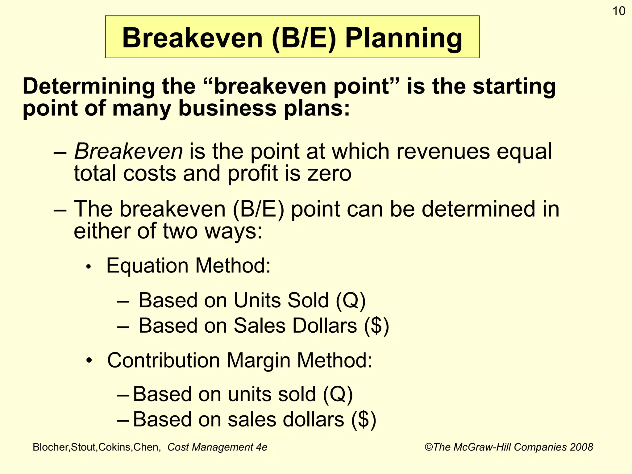
B/E Planning (continued)
The Equation Methods (@ B/E, N = $0)
1) B/E in unit sales (Q = sales in units):
p x Q = (v x Q) + F + N
p x Q = (v x Q) + F
F = total fixed cost, N = operating profit
2) B/E in sales dollars (Y = sales in dollars) :
Y = [(v/p) x Y ] + F + N
Y = [(v/p) x Y ] + F](https://image.slidesharecdn.com/6cvpanlysisnew-230404131851-d700c3ea/75/6-CVP-anlysis-NEW-pptx-11-2048.jpg)


![Blocher,Stout,Cokins,Chen, Cost Management 4e ©The McGraw-Hill Companies 2008
15
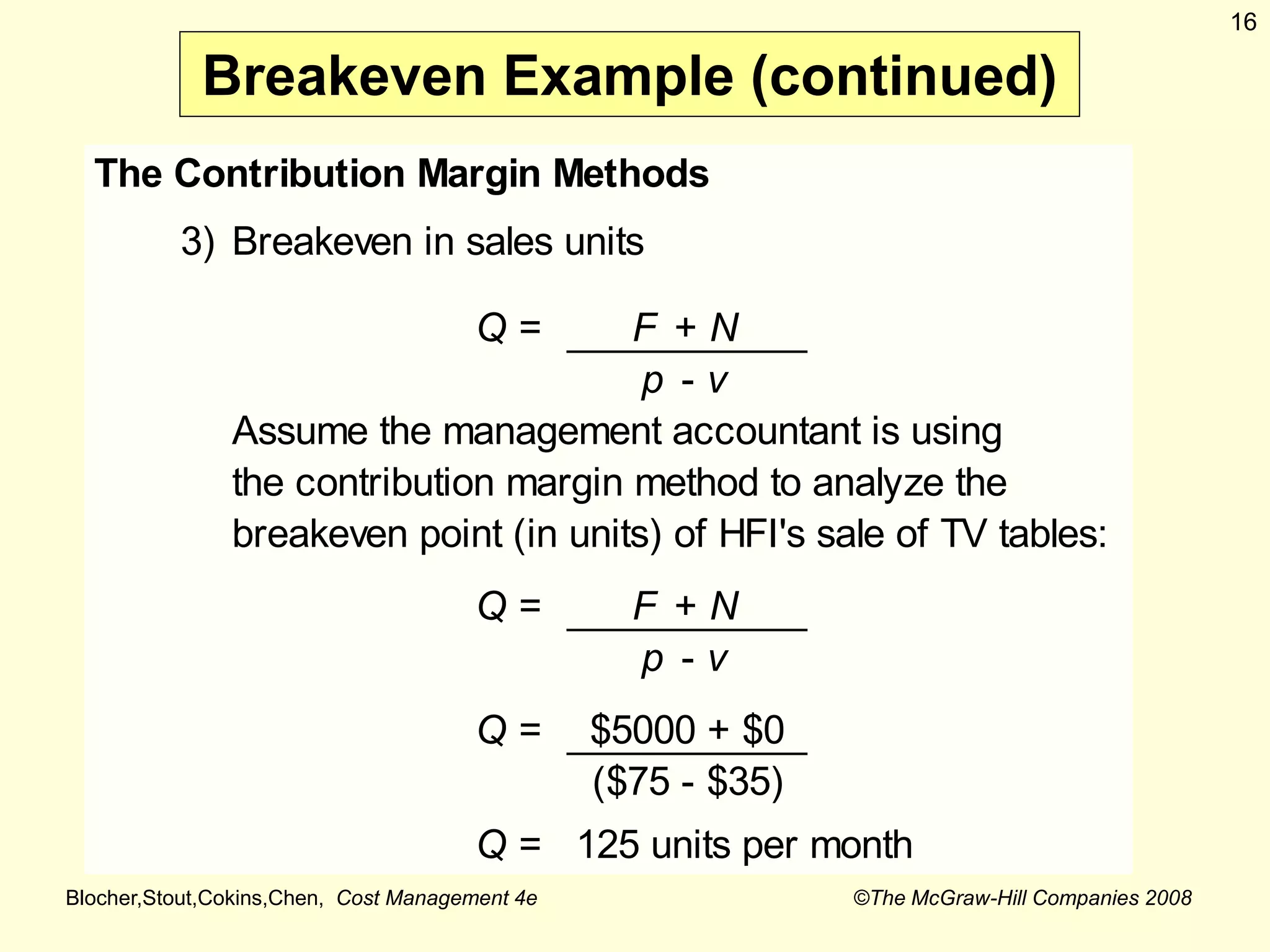
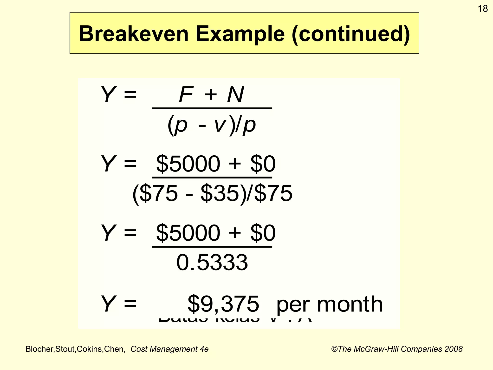
Breakeven Example (continued)
The Equation Methods (Continued)
2) Breakeven in sales dollars (Y = sales in dollars)
Y = [(v/p) x Y] + F + N
Assume the management accountant is using the equation method
to analyze the breakeven point (in sales dollars) of HFI's sale of TV tables
and he/she does not know the unit sales price or the unit variable costs:
Y = [(v/p) x Y] + F + N
Y = [($84,000/$180,000) x Y] + $5,000 + $0
Y = [0.4667 x Y] + $5,000
Y = $9,375 per month
$ 13.927,5](https://image.slidesharecdn.com/6cvpanlysisnew-230404131851-d700c3ea/75/6-CVP-anlysis-NEW-pptx-15-2048.jpg)