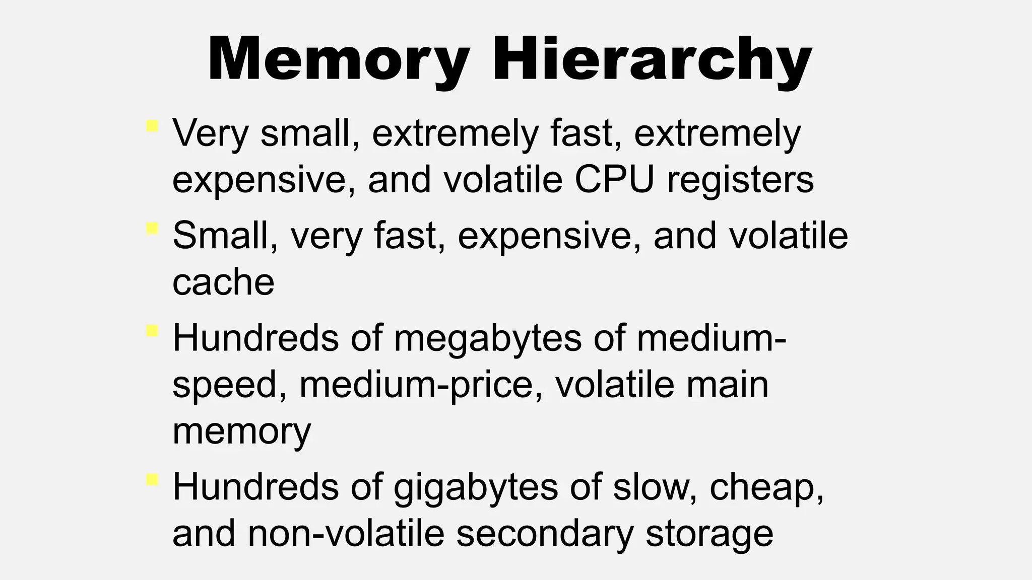
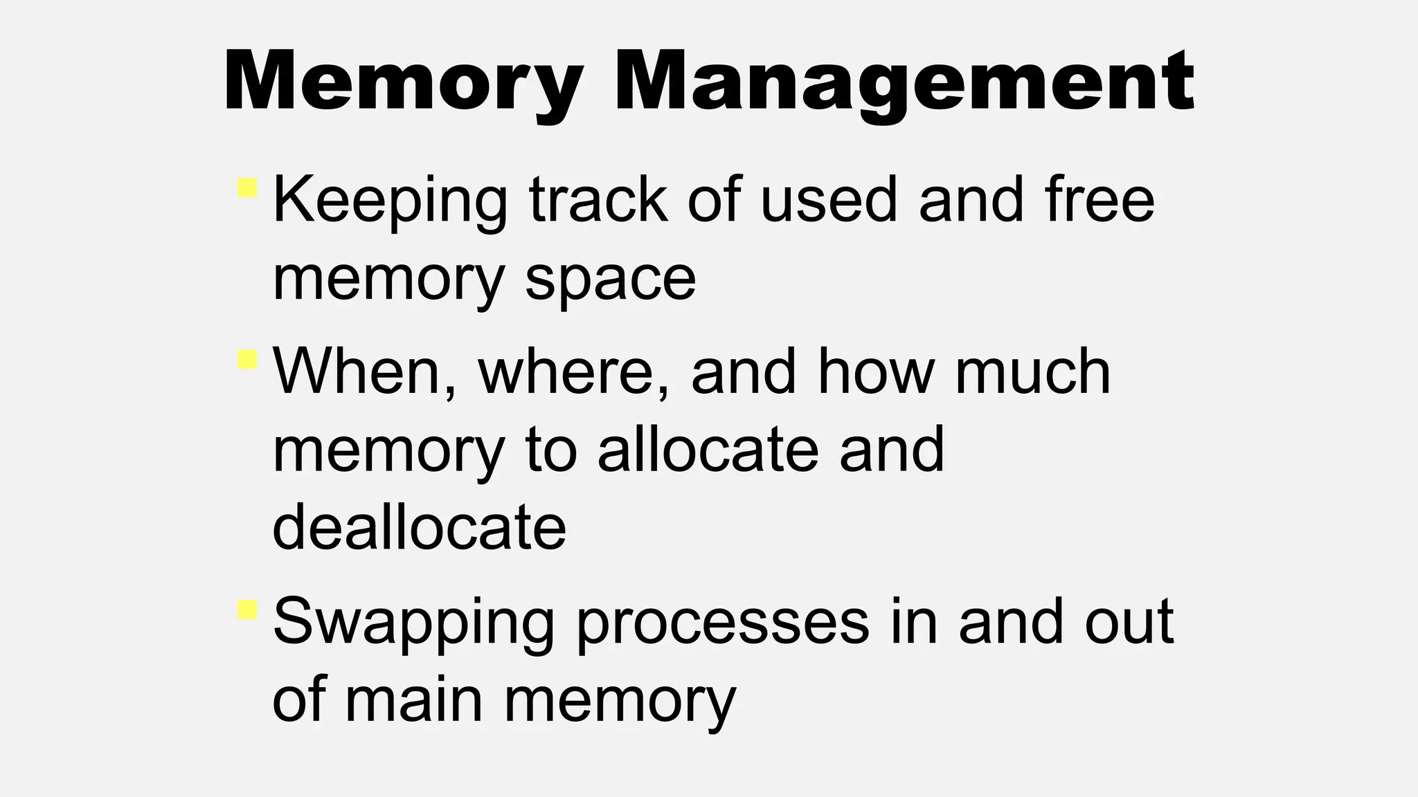
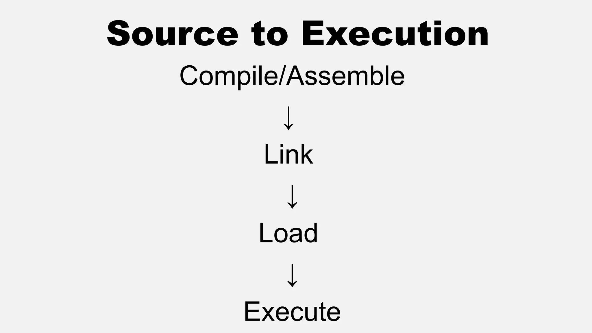
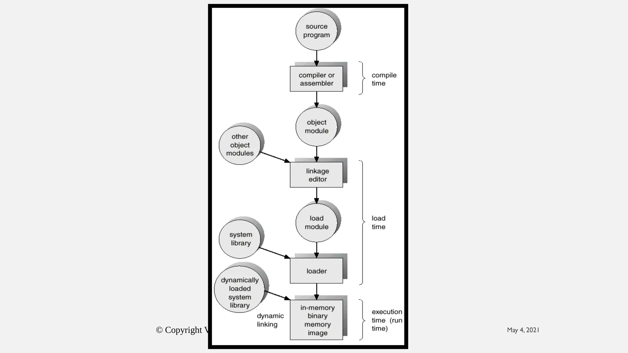
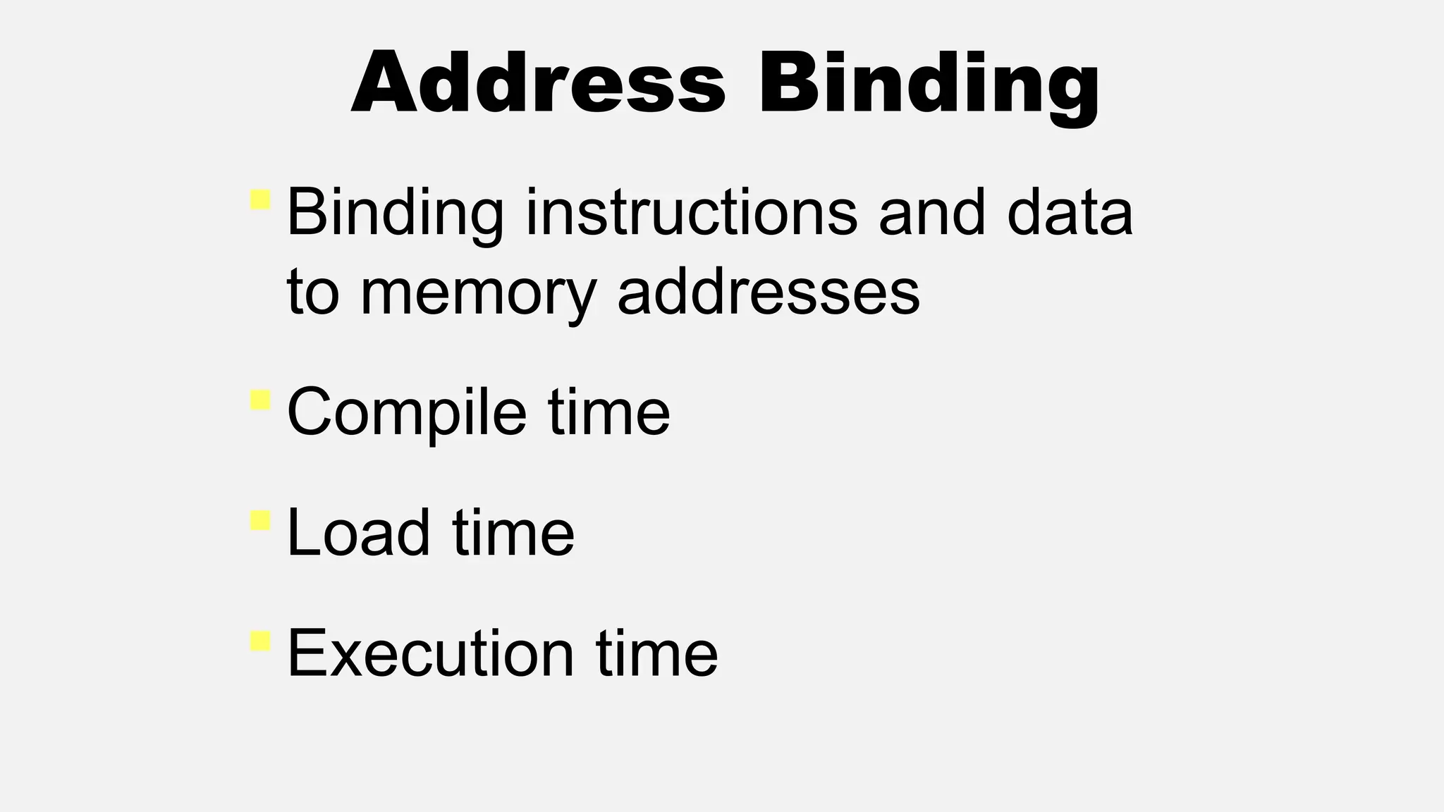
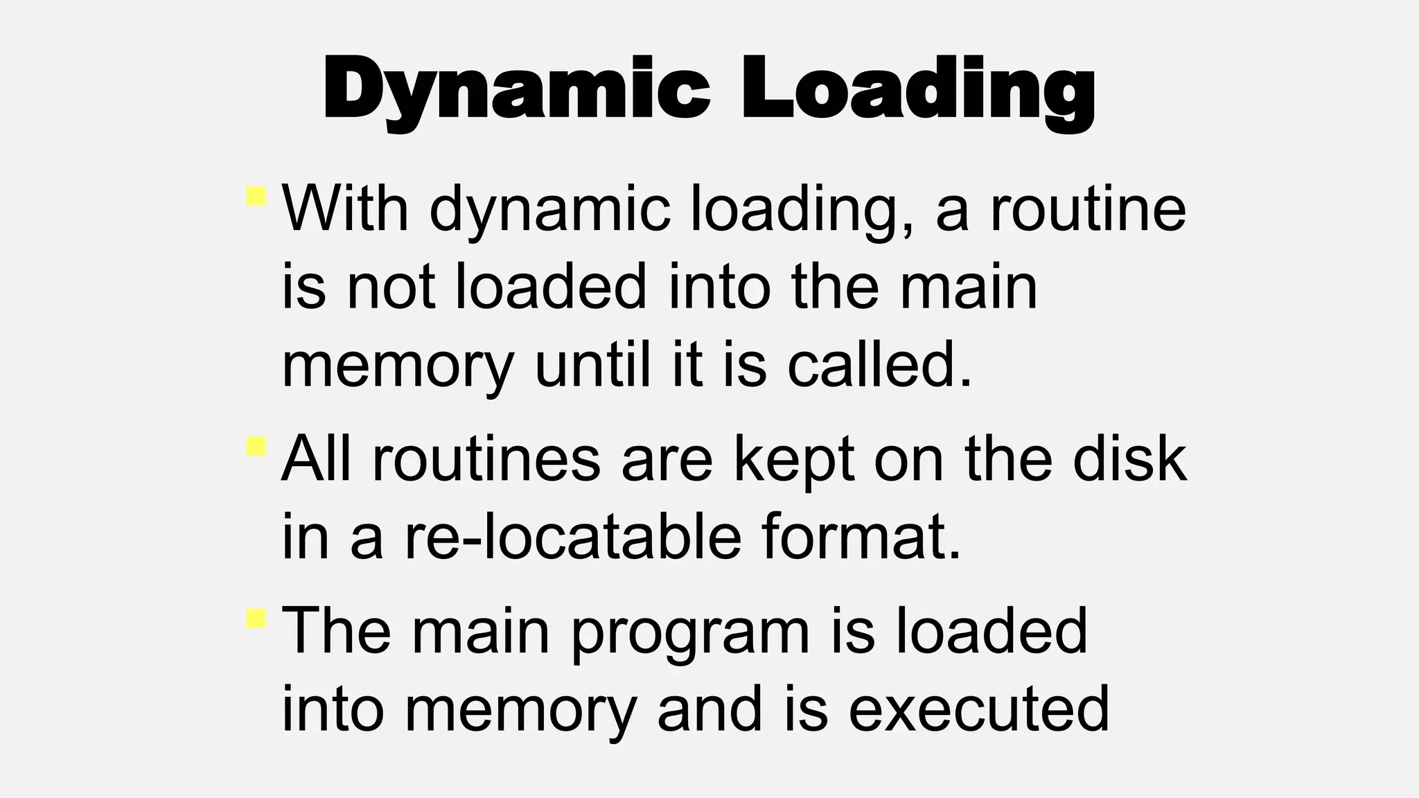
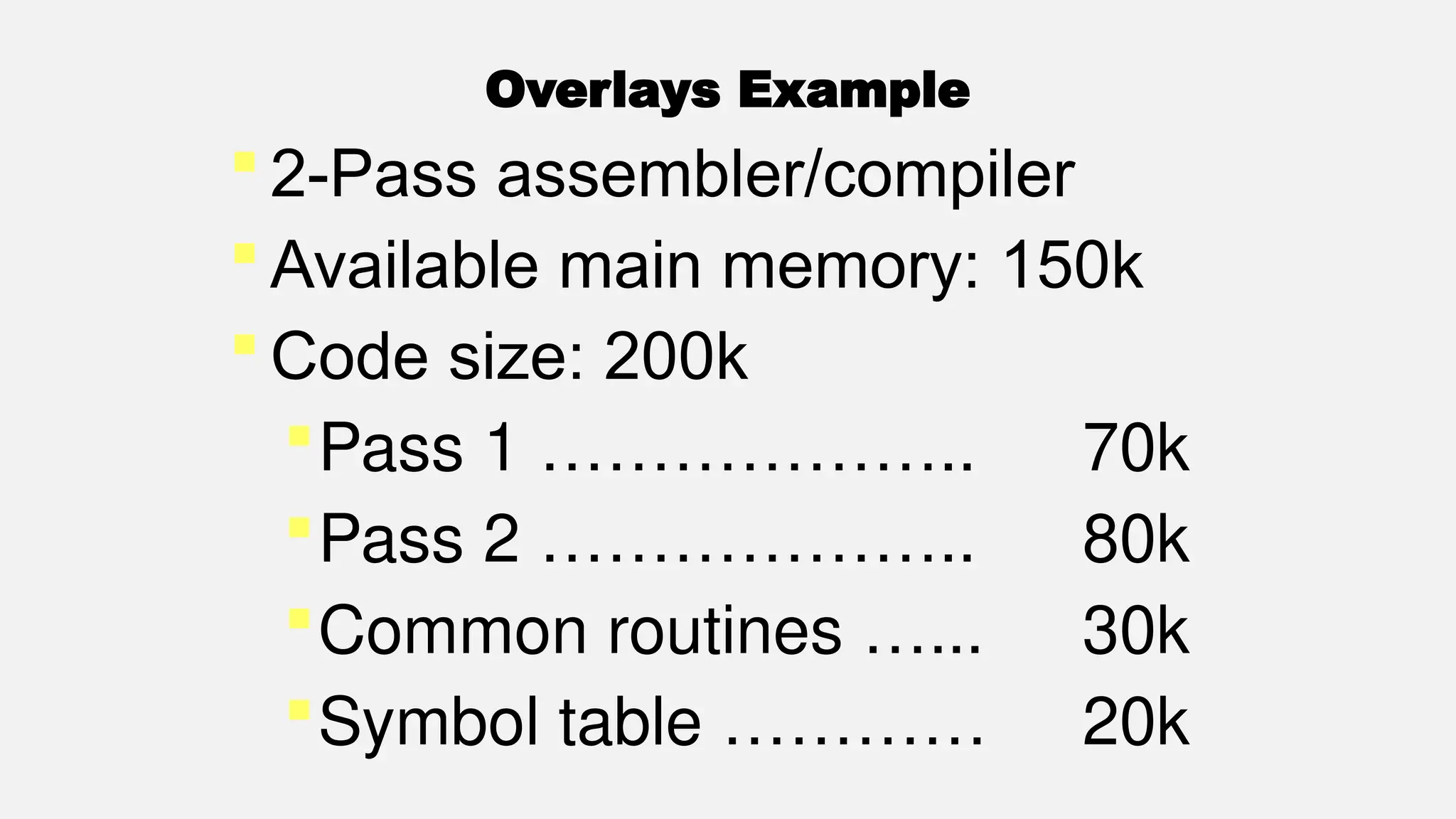
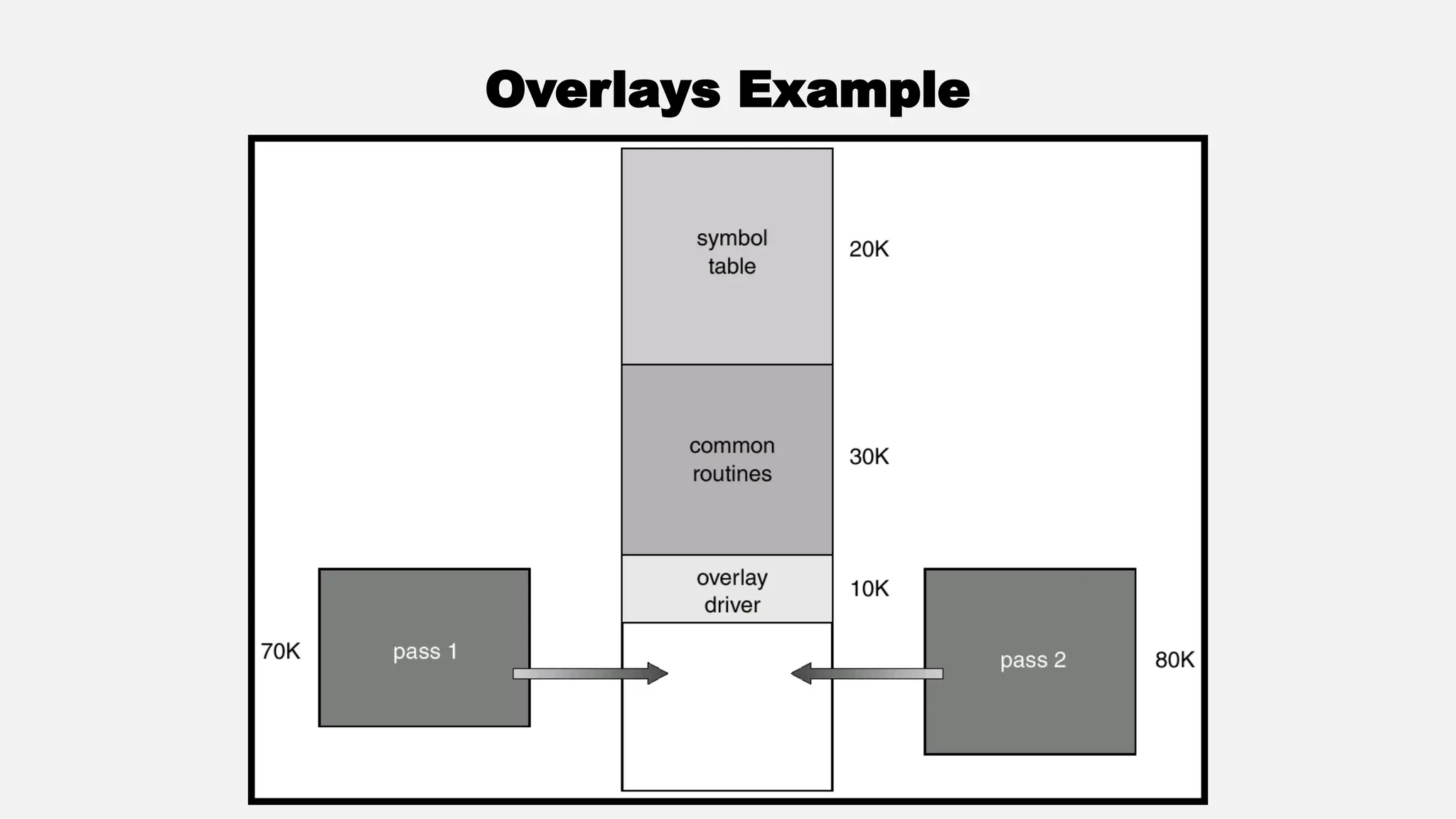
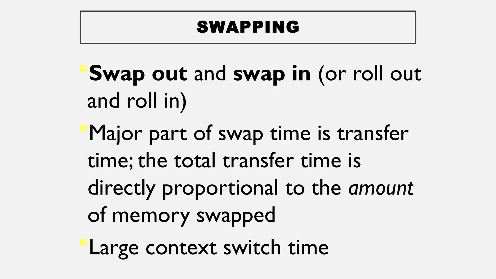
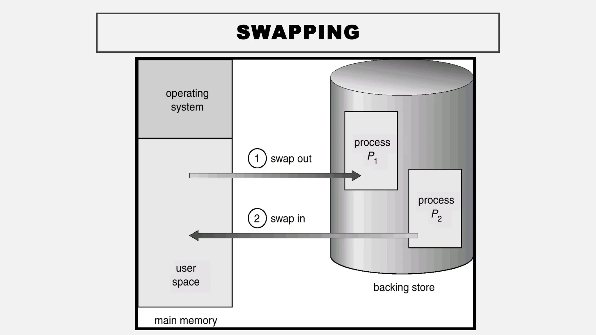
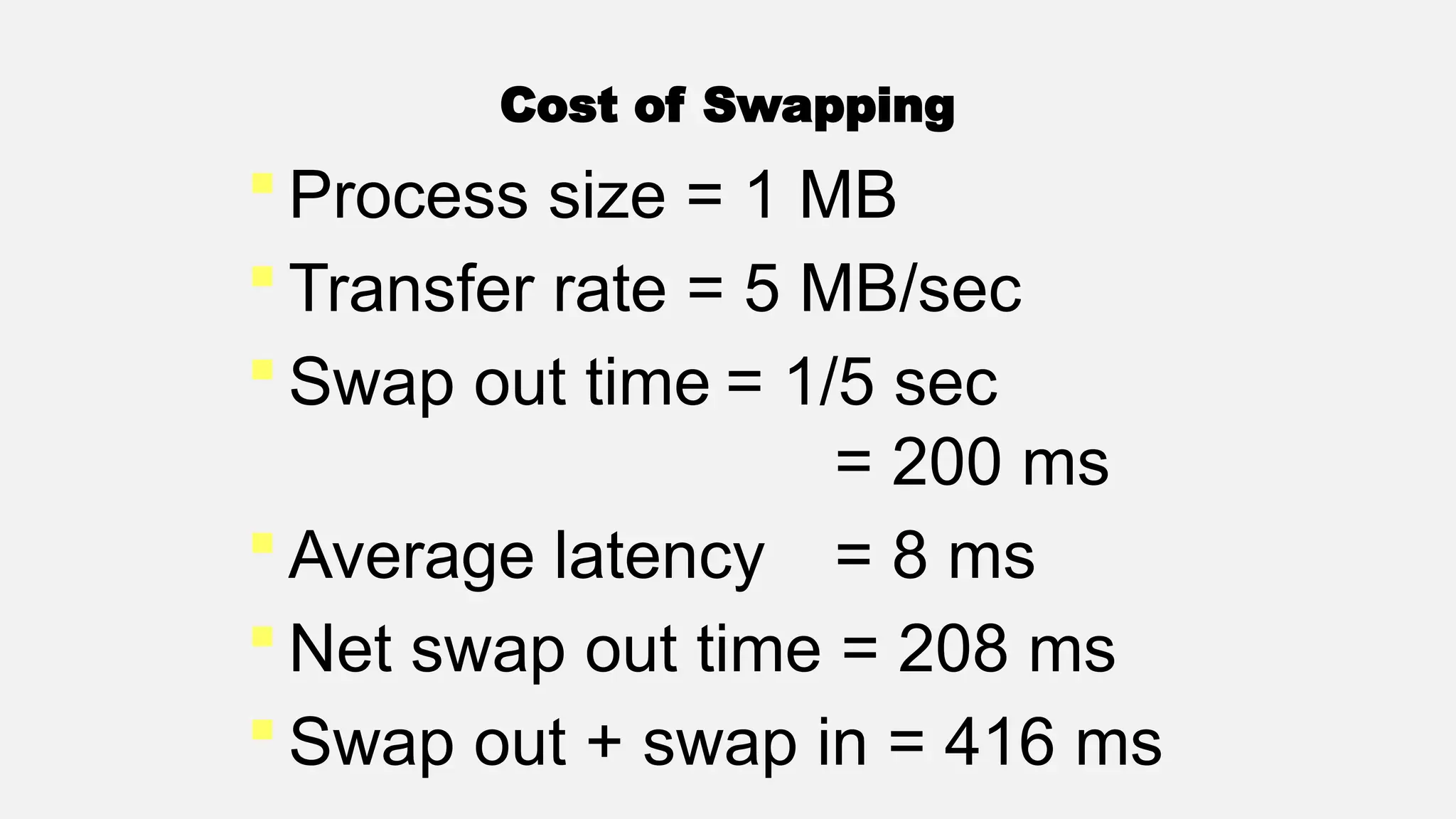
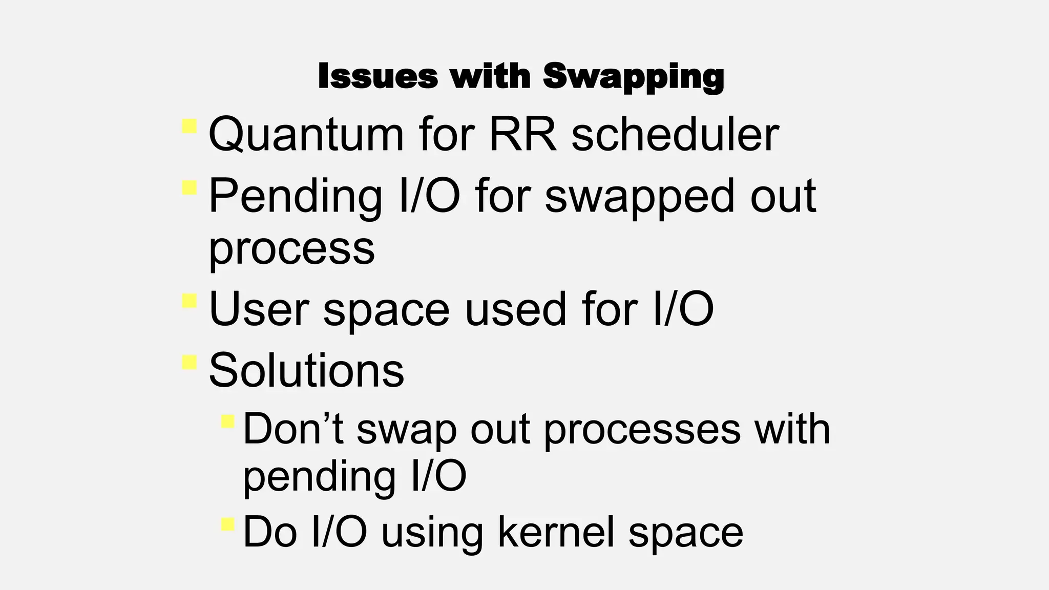
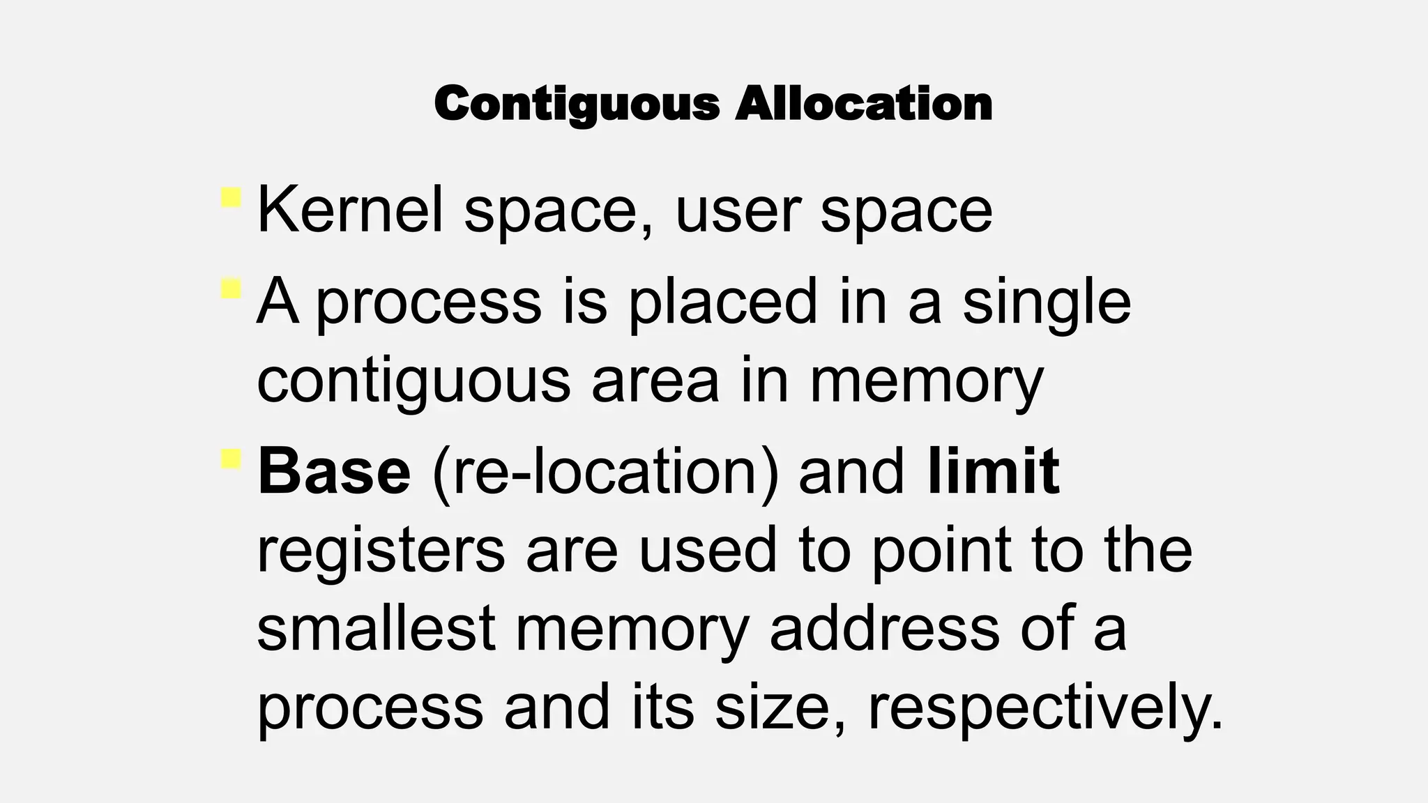
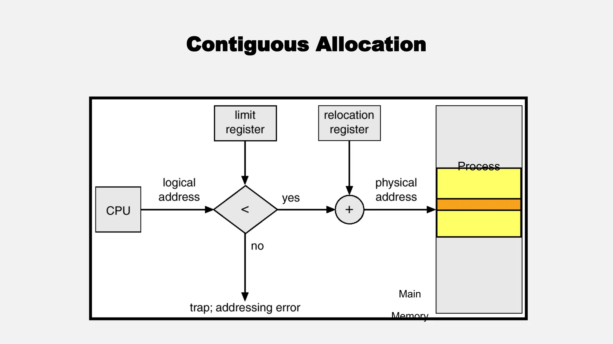
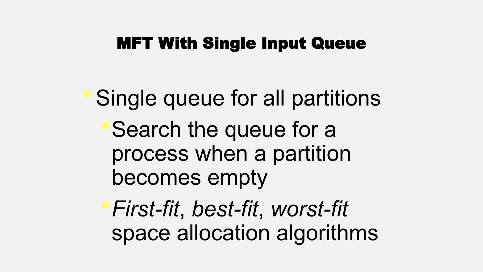
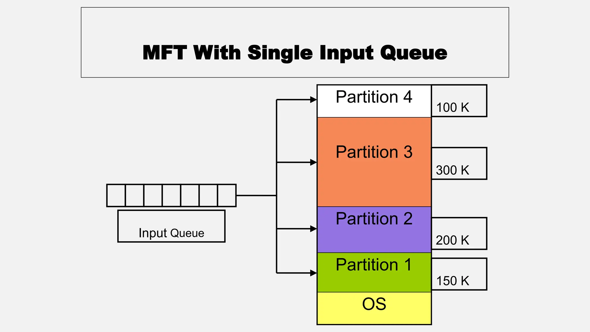
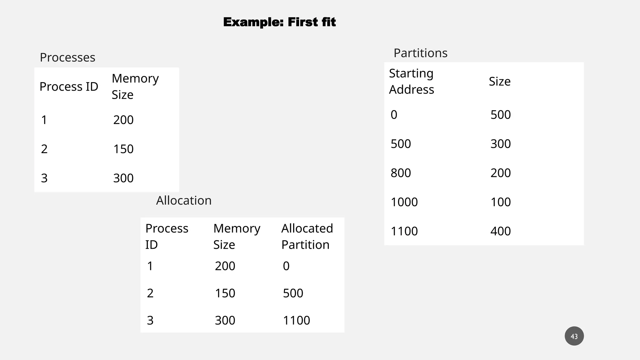
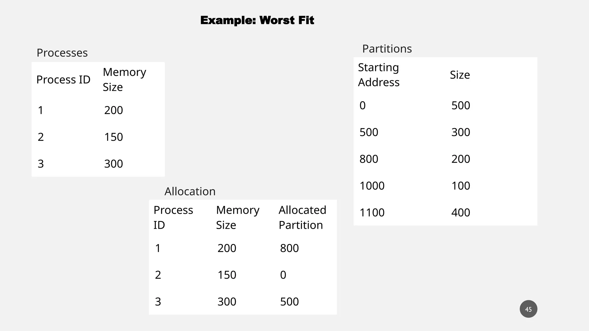
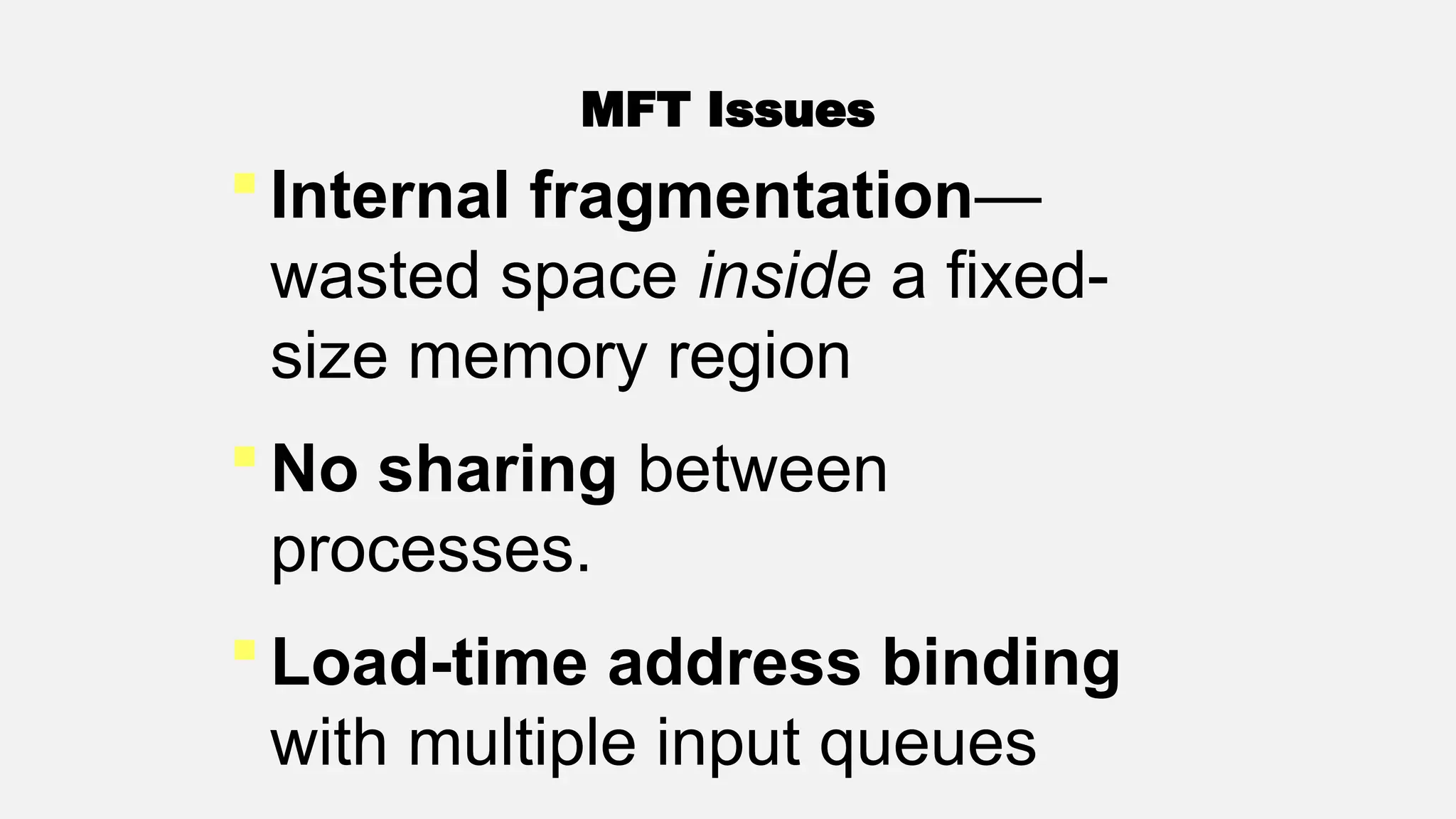
The document discusses memory management in operating systems, covering topics such as address binding, logical and physical address spaces, and memory hierarchy. It explains techniques like dynamic loading, dynamic linking, and overlays to optimize memory use during program execution. Additionally, concepts related to swapping processes and memory allocation strategies are explored, alongside practical examples of memory partitioning techniques.

1. OPERATING SYSTEMS
(CSC 2205)
Instructor: Mr. Khwaja Bilal Hassan
BS CS UET Peshawar
M.Phil. CS Quaid-e-Azam University Islamabad
Lecture#12
Memory Management
1

2. Agenda for Today
 What is memory management
 Source code to execution
 Address binding
 Logical and physical address spaces
 Dynamic loading, dynamic linking,
and overlays

3. Memory Hierarchy
 Very small, extremely fast, extremely
expensive, and volatile CPU registers
 Small, very fast, expensive, and volatile
cache
 Hundreds of megabytes of medium-
speed, medium-price, volatile main
memory
 Hundreds of gigabytes of slow, cheap,
and non-volatile secondary storage

4. Purpose of Memory
Management
To ensure fair, secure,
orderly, and efficient use
of memory

5. Memory Management
Keeping track of used and free
memory space
When, where, and how much
memory to allocate and
deallocate
Swapping processes in and out
of main memory

6. Source to Execution
Compile/Assemble
↓
Link
↓
Load
↓
Execute

7. © Copyright Virtual University of Pakistan May 4, 2021

8.  Binding instructions and data
to memory addresses
 Compile time
 Load time
 Execution time
Address Binding

9.  Compile time: If you know at
compile time where the
process will reside in memory,
the absolute code can be
generated. Process must
reside in the same memory
region for it to execute
correctly.
Address Binding

10.  Load time: If the location of a
process in memory is not known
at compile time, then the
compiler must generate re-
locatable code. In this case the
final binding is delayed until load
time. Process can be loaded in
different memory regions.
Address Binding

11. Address Binding
 Execution time: If the process
can be moved during its
execution from one memory
region to another, then binding
must be delayed until run time.
Special hardware must be
available for this to work.

12. Logical and Physical
Addresses
 Logical address: An address
generated by the process/CPU;
refers to an instruction or data in
the process
 Physical address: An address for
a main memory location where
instruction or data resides

13. Logical and Physical
Address Spaces
 The set of all logical addresses
generated by a process comprises
its logical address space.
 The set of physical addresses
corresponding to these logical
addresses comprises the physical
address space for the process.

14. Logical and Physical
Address Spaces
 The run-time mapping from
logical to physical addresses is
done by a piece of the CPU
hardware, called the memory
management unit (MMU).

15. Example
 The base register is called the
relocation register.
 The value in the relocation
register is added to every
address generated by a user
process at the time it is sent to
memory.

16. Example
14000
Process

17. Example
 In i8086, the logical address of
the next instruction is specified by
the value of instruction pointer
(IP). The physical address for the
instruction is computed by shifting
the code segment register (CS)
left by four bits and adding IP to it.

18. Example
CPU
CS * 24
+
MMU
Logical
address
Physical
address

19. Example
 Logical address (16-bit)
IP = 0B10h
CS = D000h
 Physical address (20-bit)
CS * 24
+ IP = D0B10h
 Sizes of logical and physical
address spaces?

20. Dynamic Loading
With dynamic loading, a routine
is not loaded into the main
memory until it is called.
All routines are kept on the disk
in a re-locatable format.
The main program is loaded
into memory and is executed

21. Dynamic Loading
Advantages
Potentially less time needed to
load a program
Potentially less memory space
needed
Disadvantage
Run-time activity

22. Dynamic Linking
In static linking, system
language libraries are linked
at compile time and, like any
other object module, are
combined by the loader into
the binary image

23. Dynamic Linking
 In dynamic linking, linking is
postponed until run-time.
 A library call is replaced by a
piece of code, called stub,
which is used to locate
memory-resident library routine

24. Dynamic Linking
During execution of a process,
stub is replaced by the address
of the relevant library code and
the code is executed
If library code is not in memory,
it is loaded at this time

25. Dynamic Linking
Advantages
Potentially less time needed to
load a program
Potentially less memory space
needed
Less disk space needed to
store binaries

26. Dynamic Linking
Disadvantages
Time-consuming run-time activity,
resulting in slower program
execution
gcc compiler
Dynamic linking by default
-static option allows static
linking

27. Overlays
 Allow a process to be larger
than the amount of memory
allocated to it
 Keep in memory only those
instructions and data that are
needed at any given time

28. Overlays
 When other instructions are
needed, they are loaded into the
space occupied previously by
instructions that are no longer
needed
 Implemented by user
 Programming design of overlay
structure is complex and not
possible in all cases

29. Overlays Example
 2-Pass assembler/compiler
 Available main memory: 150k
 Code size: 200k
Pass 1 ……………….. 70k
Pass 2 ……………….. 80k
Common routines …... 30k
Symbol table ………… 20k

30. Overlays Example

31. SWAPPING
Swap out and swap in (or roll out
and roll in)
Major part of swap time is transfer
time; the total transfer time is
directly proportional to the amount
of memory swapped
Large context switch time

32. SWAPPING

33. Cost of Swapping
 Process size = 1 MB
 Transfer rate = 5 MB/sec
 Swap out time = 1/5 sec
= 200 ms
 Average latency = 8 ms
 Net swap out time = 208 ms
 Swap out + swap in = 416 ms

34. Issues with Swapping
 Quantum for RR scheduler
 Pending I/O for swapped out
process
 User space used for I/O
 Solutions
Don’t swap out processes with
pending I/O
Do I/O using kernel space

35. Contiguous Allocation
 Kernel space, user space
 A process is placed in a single
contiguous area in memory
 Base (re-location) and limit
registers are used to point to the
smallest memory address of a
process and its size, respectively.

36. Contiguous Allocation
Main
Memory
Process

37. MFT
 Multiprogramming with fixed
tasks (MFT)
 Memory is divided into several
fixed-size partitions.
 Each partition may contain
exactly one process/task.

38. MFT
 Boundaries for partitions are set
at boot time and are not
movable.
 An input queue per partition
 The degree of multiprogramming
is bound by the number of
partitions.

39. Partition 4
Partition 3
Partition 2
Partition 1
OS
MFT
100 K
300 K
200 K
150 K
Input
Queues

40.  Potential for wasted memory
space—an empty partition but
no process in the associated
queue
 Load-time address binding
MFT With Multiple Input Queues

41.  Single queue for all partitions
Search the queue for a
process when a partition
becomes empty
First-fit, best-fit, worst-fit
space allocation algorithms
MFT With Single Input Queue

42. Partition 4
Partition 3
Partition 2
Partition 1
OS
100 K
300 K
200 K
150 K
Input Queue
MFT With Single Input Queue

43. 43
Process ID
Memory
Size
1 200
2 150
3 300
Starting
Address
Size
0 500
500 300
800 200
1000 100
1100 400
Processes
Example: First fit
Partitions
Process
ID
Memory
Size
Allocated
Partition
1 200 0
2 150 500
3 300 1100
Allocation

44. 44
Process
ID
Memory
Size
Allocated
Partition
1 200 800
2 150 500
3 300 1100
Process ID
Memory
Size
1 200
2 150
3 300
Starting
Address
Size
0 500
500 300
800 200
1000 100
1100 400
Processes
Example: Best fit
Partitions
Allocation

45. 45
Process
ID
Memory
Size
Allocated
Partition
1 200 800
2 150 0
3 300 500
Process ID
Memory
Size
1 200
2 150
3 300
Starting
Address
Size
0 500
500 300
800 200
1000 100
1100 400
Processes
Example: Worst Fit
Partitions
Allocation

46.  Internal fragmentation—
wasted space inside a fixed-
size memory region
 No sharing between
processes.
 Load-time address binding
with multiple input queues
MFT Issues