This document discusses forgotten trigonometric functions that were used for navigation before GPS. It describes the versine and haversine functions, which are related to cosine and were used in navigation calculations. The haversine formula allowed early navigators to calculate distances between locations given their latitudes and longitudes, enabling navigation without modern technologies.

1. The
Forgotten
Trigonometric
Functions,
or
How
Trigonometry
was
used
in
the
Ancient
Art
of
Navigation
(Before
GPS!)
Recently,
as
I
was
exploring
some
mathematical
concept
I
came
across
some
terms
that
were
suspiciously
similar
to
some
familiar
trigonometric
functions.
What
is
an
excosecant?
How
about
a
Havercosine?
As
it
turns
out,
these
belong
to
a
family
of
trigonometric
functions
that
once
enjoyed
very
standard
usage,
in
very
notable
and
practical
fields,
but
in
recent
times
have
become
nearly
obsolete.
Versine
The
most
basic
of
this
family
of
functions
is
the
versine,
or
versed
sine.
The
versine,
abbreviated
versin
of
some
angle
x
is
actually
calculated
by
subtracting
the
cosine
of
x
from
1;
that
is
versin(x)
=
1
-­‐
cos
(x).
Through
some
manipulations
with
half-­‐
angle
identities,
we
can
see
another
equivalent
expression:
Notice,
we
do
not
need
the
±
as
the
versine
will
always
represent
non-­‐negative
value
(since
cosine
ranges
from
negative
one
to
positive
one,
one
minus
these
values
will
range
from
zero
to
two).
This
was
especially
helpful
as
navigators
used
logarithms
in
their
calculations,
so
they
could
always
take
the
logarithm
of
the
versine.
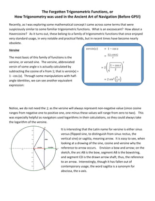
It
is
interesting
that
the
Latin
name
for
versine
is
either
sinus
versus
(flipped
sine,
to
distinguish
from
sinus
rectus,
the
vertical
sine)
or
sagitta,
meaning
arrow.
It
is
easy
to
see,
when
looking
at
a
drawing
of
the
sine,
cosine
and
versine
why
the
reference
to
arrow
occurs.
Envision
a
bow
and
arrow;
on
the
sketch,
the
arc
AB
is
the
bow,
segment
AB
is
the
bowstring,
and
segment
CD
is
the
drawn
arrow
shaft,
thus,
the
reference
to
an
arrow.
Interestingly,
though
it
has
fallen
out
of
contemporary
usage,
the
word
sagitta
is
a
synonym
for
abscissa,
the
x-­‐axis.
!"#$%&(!)
= 1 − cos !
=
!(!!!"#!)
!
= 2 !!
1 − cos !
2
!
!
= 2 !"#! !
1
2
!!

2. !"#$%& ! = 1 − cos ! = 2 !"#! !
1
2
!!
ℎ!"#$%&' ! =
1 − cos !
2
= !"#! !
1
2
!!
!"# ! = 1 − !"#$%& ! = 1 − 2 ℎ!"#$%&' !
Haversine
While
this
function
is
obviously
related
to
the
versine
(literally,
it
is
half
the
versine,
thus
haversine),
it
has
the
most
practical
usage
associated
with
it.
In
early
times,
navigators
would
calculate
distance
from
their
known
latitudinal
and
longitudinal
coordinates
to
those
of
their
desired
destination
by
using
what
became
known
as
the
Haversine
formula.
Starting
with
the
Spherical
Law
of
Cosines,
and
making
appropriate
substitutions
using
the
definition
of
haversine,
and
the
difference
of
cosines
identity,
we
can
derive
what
is
known
as
the
Law
of
Haversines.
From
there,
we
can
relate
it
to
the
specific
case
of
the
earth
to
arrive
at
the
Haverine
formula,
which
then
can
be
applied
to
find
a
distance
between
two
points.
!"#$%$&' !"# !"# !" !"#$%&'($&:
!ℎ! !"ℎ!"#$%& !"# !" !"#$%&#:
cos ! = cos ! cos ! + sin ! sin ! cos!
Where
a,
b,
c
are
spherical
arcs,
and
C
is
the
spherical
angle
between
a
and
b.
First,
substitute
for
cos
c
and
cos
C
in
terms
of
haversine:
1 − 2 hav ! = cos ! cos ! + sin ! sin !(1 − 2 hav !)
Then
distributing
on
the
right
hand
side:
1 − 2 hav ! = cos ! cos ! + sin ! sin ! − 2 sin ! sin ! ℎ!" !
Replacing
the
difference
of
cosines:
1 − 2 hav ! = cos(! − !) − 2 sin ! sin ! ℎ!" !
Next,
substitute
for
cos
(a-­‐b)
in
terms
of
haversin:
1 − 2 hav ! = 1 − 2 hav(! − !) − 2 sin ! sin ! ℎ!" !
Last,
simplify
by
subtracting
one
and
dividing
by
-­‐2:
hav ! = hav(! − !) + sin ! sin ! ℎ!" !

3. So,
now
we
are
able
to
determine
the
distance
between
two
points.
Letting
point
1
be
Atlanta,
GA
(33o
44’56”N,
84o
23’17”W)
and
point
2
be
Sao
Paulo,
Brazil
(23o
32’0”S,
46o
37’0”W),
we
should
be
able
to
find
the
distance
by
making
appropriate
substitutions
and
a
reasonable
approximation
for
the
radius
of
the
earth
(which
is
not
a
perfect
sphere).
We
will
use
the
mean
of
the
shortest
and
longest
radii:
approximately
3959
miles.
Check
out
the
link
on
my
home
page
for
an
Excel
Worksheet
that
will
calculate
the
distance
between
two
locations
using
the
Haversine
Formula
and
their
latitudes
and
longitudes.
!"#$ !"# !"# !" !"#$%&'($& !" !"# !"#$%&'($ !"#$%&':
hav ! = hav(! − !) + sin ! sin ! ℎ!" !
Let
d
be
the
spherical
distance
between
any
two
points
on
the
surface
of
the
earth,
r
be
the
radius
of
the
earth,
∝! !"! ∝!
be
the
latitudes
of
point
1
and
point
2,
respectively,
and
!! !"# !!
be
their
respective
longitudes.
The
haversine
of
the
central
angle
between
the
points
is:
hav !
!
!
! = hav(∝!−∝!) + cos ∝! cos ∝! ℎ!" (!! − !!)
Since
ℎ!"#$%&' ! = !"#! !
!
!
!!,
we
have
!"#! !
!
2!
! = hav(∝!−∝!) + cos ∝! cos ∝! ℎ!" (!! − !!)
And
!
!!
= !"#$%&! hav(∝!−∝!) + cos ∝! cos ∝! ℎ!" (!! − !!)
Finally,
! = 2! !"#$%&!!"#! !
∝!!∝!
!
! + cos ∝! cos ∝! !"#! !
!!!!!
!
!
!"#$% !"# !"#$%&'($ !"#$%&':
! = 2(3959) !"#$%&!!"#! !
−23.533° − 33.749°
2
! + cos 33.749° cos(−23.533°) !"#! !
46.617° − 84.388°
2
!
! = 7918 !"#$%&!!"#!(−28.641°) + cos33.749° cos(−23.533°) !"#! (−18.886)
! = 7918 !"#$%&!(−0.4793)! + (0.8315)(0.9168)(−0.3237)!
! = 7918 !"#$%&√. 3096
! = 7918 !"#$%& 0.5564
! = 7918 (33.8083) !
!
180
! ≈ 4672 !"#$%

4. There
are
many
other
“classical”
trigonometric
functions
that
are
not
as
practical
and
have
been
abandoned
in
favor
of
manipulation
of
the
six
well-­‐known
(and
loved)
trig
ratios.
The
table
and
diagram
below
illustrate
how
these
functions
are
defined.
As
we
evolve
technologically,
it
is
important
that
we
remember
and
recall
the
steps
we
have
taken
to
achieve
the
stature
we
have
reached
thus
far.
It
is
valuable
for
us
to
remember
those
“giants”
upon
whose
shoulders
we
happen
to
currently
stand.
Weisstein,
Eric
W.
"Versine."
From
MathWorld-­‐-­‐A
Wolfram
Web
Resource.
http://mathworld.wolfram.com/Versine.html
http://en.wikipedia.org/wiki/Versine
http://en.wikipedia.org/wiki/Haversine_formula
Kells,
Kern
&
Bland.
Plane
and
Spherical
Trigonometry.
York,
PA:
Maple
Press
Company,
1935.
Print.
!"#$%&'(" ! 1 + !"#$%& !
!"#$%&'($ ! 1 − !"#$ !
!"#$%!"&'($ ! 1 + !"#$ !
ℎ!"#$%&'()# ! 1 + !"#$%& !
2
ℎ!!"#$%&'($ ! 1 − !"#$ !
2
ℎ!"#$%&"#'()% ! 1 + !"#$ !
2
!"#!"#$% ! !"#$%& ! − 1
!"#$%!#&'( ! !"#$!%&' ! − 1