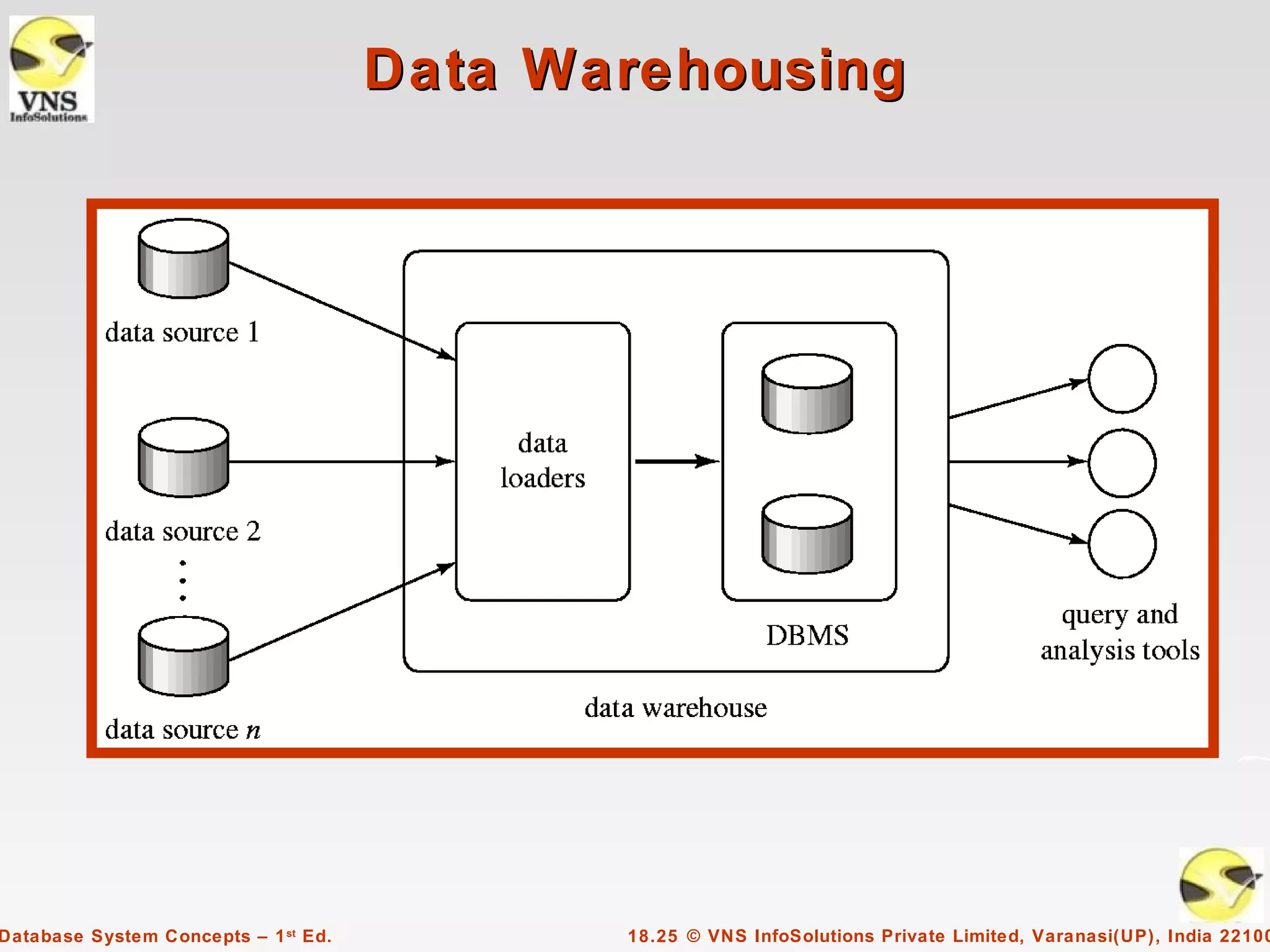
SlideShare a Scribd company logo
Chapter 18: Data Analysis and
           Mining


          Database System Concepts, 1 st Ed.
  ©VNS InfoSolutions Private Limited, Varanasi(UP), India 221002
          See www.vnsispl.com for conditions on re-use
Chapter 18: Data Analysis and Mining

               s Decision Support Systems
               s Data Analysis and OLAP
               s Data Warehousing
               s Data Mining


Database System Concepts – 1 st Ed.         18.2 © VNS InfoSolutions Private Limited, Varanasi(UP), India 22100
Decision Support Systems

               s Decision-support systems are used to make business decisions, often
                    based on data collected by on-line transaction-processing systems.
               s Examples of business decisions:
                      q   What items to stock?
                      q   What insurance premium to change?
                      q   To whom to send advertisements?
               s Examples of data used for making decisions
                      q      Retail sales transaction details
                      q      Customer profiles (income, age, gender, etc.)


Database System Concepts – 1 st Ed.                    18.3 © VNS InfoSolutions Private Limited, Varanasi(UP), India 22100
Decision-Support Systems: Overview
           s Data analysis tasks are simplified by specialized tools and SQL
                extensions
                 q   Example tasks
                          For each product category and each region, what were the total
                           sales in the last quarter and how do they compare with the same
                           quarter last year
                          As above, for each product category and each customer category
           s Statistical analysis packages (e.g., : S++) can be interfaced with
                databases
                 q   Statistical analysis is a large field, but not covered here
           s Data mining seeks to discover knowledge automatically in the form of
                statistical rules and patterns from large databases.
           s A data warehouse archives information gathered from multiple sources,
                and stores it under a unified schema, at a single site.
                 q   Important for large businesses that generate data from multiple
                     divisions, possibly at multiple sites
                 q   Data may also be purchased externally


Database System Concepts – 1 st Ed.                  18.4 © VNS InfoSolutions Private Limited, Varanasi(UP), India 22100
Data Analysis and OLAP
             s Online Analytical Processing (OLAP)
                    q   Interactive analysis of data, allowing data to be summarized and
                        viewed in different ways in an online fashion (with negligible delay)
             s Data that can be modeled as dimension attributes and measure
                  attributes are called multidimensional data.
                    q   Measure attributes
                            measure some value
                            can be aggregated upon
                            e.g. the attribute number of the sales relation
                    q   Dimension attributes
                            define the dimensions on which measure attributes (or
                             aggregates thereof) are viewed
                            e.g. the attributes item_name, color, and size of the sales
                             relation


Database System Concepts – 1 st Ed.                    18.5 © VNS InfoSolutions Private Limited, Varanasi(UP), India 22100
Cross Tabulation of sales by item-
                         name and color


      s The table above is an example of a cross-tabulation (cross-tab), also
           referred to as a pivot-table.
             q   Values for one of the dimension attributes form the row headers
             q   Values for another dimension attribute form the column headers
             q   Other dimension attributes are listed on top
             q   Values in individual cells are (aggregates of) the values of the
                 dimension attributes that specify the cell.

Database System Concepts – 1 st Ed.                18.6 © VNS InfoSolutions Private Limited, Varanasi(UP), India 22100
Relational Representation of Cross-
                              tabs

      s Cross-tabs can be represented
           as relations
             s We use the value all is used to
                 represent aggregates
             s The SQL:1999 standard
                 actually uses null values in
                 place of all despite confusion
                 with regular null values


Database System Concepts – 1 st Ed.               18.7 © VNS InfoSolutions Private Limited, Varanasi(UP), India 22100
Data Cube
      s A data cube is a multidimensional generalization of a cross-tab
      s Can have n dimensions; we show 3 below
      s Cross-tabs can be used as views on a data cube


Database System Concepts – 1 st Ed.      18.8 © VNS InfoSolutions Private Limited, Varanasi(UP), India 22100
Online Analytical Processing
         s Pivoting: changing the dimensions used in a cross-tab is called
         s Slicing: creating a cross-tab for fixed values only
                q   Sometimes called dicing, particularly when values for multiple
                    dimensions are fixed.
         s Rollup: moving from finer-granularity data to a coarser granularity
         s Drill down: The opposite operation - that of moving from coarser-
              granularity data to finer-granularity data


Database System Concepts – 1 st Ed.                18.9 © VNS InfoSolutions Private Limited, Varanasi(UP), India 22100
Hierarchies on Dimensions
          s Hierarchy on dimension attributes: lets dimensions to be
               viewed at different levels of detail
                 5 E.g. the dimension DateTime can be used to aggregate by hour of
                   day, date, day of week, month, quarter or year


Database System Concepts – 1 st Ed.             18.10 © VNS InfoSolutions Private Limited, Varanasi(UP), India 22100
Cross Tabulation With Hierarchy
           s Cross-tabs can be easily extended to deal with hierarchies
                 5 Can drill down or roll up on a hierarchy


Database System Concepts – 1 st Ed.               18.11 © VNS InfoSolutions Private Limited, Varanasi(UP), India 22100
OLAP Implementation
         s The earliest OLAP systems used multidimensional arrays in memory to
              store data cubes, and are referred to as multidimensional OLAP
              (MOLAP) systems.
         s OLAP implementations using only relational database features are called
              relational OLAP (ROLAP) systems
         s Hybrid systems, which store some summaries in memory and store the
              base data and other summaries in a relational database, are called
              hybrid OLAP (HOLAP) systems.


Database System Concepts – 1 st Ed.             18.12 © VNS InfoSolutions Private Limited, Varanasi(UP), India 22100
OLAP Implementation (Cont.)
         s Early OLAP systems precomputed all possible aggregates in order to
              provide online response
                q   Space and time requirements for doing so can be very high
                         2n combinations of group by
                q   It suffices to precompute some aggregates, and compute others on
                    demand from one of the precomputed aggregates
                         Can compute aggregate on (item-name, color) from an aggregate
                          on (item-name, color, size)
                           – For all but a few “non-decomposable” aggregates such as
                             median
                           – is cheaper than computing it from scratch
         s Several optimizations available for computing multiple aggregates
                q   Can compute aggregate on (item-name, color) from an aggregate on
                    (item-name, color, size)
                q   Can compute aggregates on (item-name, color, size),
                    (item-name, color) and (item-name) using a single sorting
                    of the base data

Database System Concepts – 1 st Ed.                18.13 © VNS InfoSolutions Private Limited, Varanasi(UP), India 22100
Extended Aggregation in SQL:1999
      s The cube operation computes union of group by’s on every subset of the
           specified attributes
      s E.g. consider the query
                    select item-name, color, size, sum(number)
                    from sales
                    group by cube(item-name, color, size)
            This computes the union of eight different groupings of the sales relation:
              { (item-name, color, size), (item-name, color),
                (item-name, size),        (color, size),
                (item-name),              (color),
                (size),                   ()}
            where ( ) denotes an empty group by list.
      s For each grouping, the result contains the null value
           for attributes not present in the grouping.


Database System Concepts – 1 st Ed.               18.14 © VNS InfoSolutions Private Limited, Varanasi(UP), India 22100
Extended Aggregation (Cont.)
        s Relational representation of cross-tab that we saw earlier, but with null in
             place of all, can be computed by
                     select item-name, color, sum(number)
                     from sales
                     group by cube(item-name, color)
        s The function grouping() can be applied on an attribute
               q   Returns 1 if the value is a null value representing all, and returns 0 in all
                   other cases.
             select item-name, color, size, sum(number),
                  grouping(item-name) as item-name-flag,
                  grouping(color) as color-flag,
                  grouping(size) as size-flag,
             from sales
             group by cube(item-name, color, size)
        s Can use the function decode() in the select clause to replace
             such nulls by a value such as all
               q   E.g. replace item-name in first query by
                     decode( grouping(item-name), 1, ‘all’, item-name)


Database System Concepts – 1 st Ed.                  18.15 © VNS InfoSolutions Private Limited, Varanasi(UP), India 22100
Extended Aggregation (Cont.)
         s The rollup construct generates union on every prefix of specified list of
              attributes
         s E.g.
                      select item-name, color, size, sum(number)
                      from sales
                      group by rollup(item-name, color, size)
               Generates union of four groupings:
                    { (item-name, color, size), (item-name, color), (item-name), ( ) }
         s Rollup can be used to generate aggregates at multiple levels of a
              hierarchy.
         s E.g., suppose table itemcategory(item-name, category) gives the
              category of each item. Then
                        select category, item-name, sum(number)
                        from sales, itemcategory
                        where sales.item-name = itemcategory.item-name
                        group by rollup(category, item-name)
              would give a hierarchical summary by item-name and by category.


Database System Concepts – 1 st Ed.                 18.16 © VNS InfoSolutions Private Limited, Varanasi(UP), India 22100
Extended Aggregation (Cont.)
       s Multiple rollups and cubes can be used in a single group by clause
              q   Each generates set of group by lists, cross product of sets gives overall
                  set of group by lists
       s E.g.,
                    select item-name, color, size, sum(number)
                    from sales
                    group by rollup(item-name), rollup(color, size)
            generates the groupings
               {item-name, ()} X {(color, size), (color), ()}
                    = { (item-name, color, size), (item-name, color), (item-name),
                        (color, size), (color), ( ) }


Database System Concepts – 1 st Ed.                  18.17 © VNS InfoSolutions Private Limited, Varanasi(UP), India 22100
Ranking
       s Ranking is done in conjunction with an order by specification.
       s Given a relation student-marks(student-id, marks) find the rank of each
            student.
            select student-id, rank( ) over (order by marks desc) as s-rank
            from student-marks
       s An extra order by clause is needed to get them in sorted order
            select student-id, rank ( ) over (order by marks desc) as s-rank
            from student-marks
            order by s-rank
       s Ranking may leave gaps: e.g. if 2 students have the same top mark, both
            have rank 1, and the next rank is 3
              q   dense_rank does not leave gaps, so next dense rank would be 2


Database System Concepts – 1 st Ed.               18.18 © VNS InfoSolutions Private Limited, Varanasi(UP), India 22100
Ranking (Cont.)
         s Ranking can be done within partition of the data.
         s “Find the rank of students within each section.”
              select student-id, section,
                   rank ( ) over (partition by section order by marks desc)
                     as sec-rank
              from student-marks, student-section
              where student-marks.student-id = student-section.student-id
              order by section, sec-rank
         s Multiple rank clauses can occur in a single select clause
         s Ranking is done after applying group by clause/aggregation


Database System Concepts – 1 st Ed.            18.19 © VNS InfoSolutions Private Limited, Varanasi(UP), India 22100
Ranking (Cont.)
             s Other ranking functions:
                    q   percent_rank (within partition, if partitioning is done)
                    q   cume_dist (cumulative distribution)
                             fraction of tuples with preceding values
                    q   row_number (non-deterministic in presence of duplicates)
             s SQL:1999 permits the user to specify nulls first or nulls last
                   select student-id,
                         rank ( ) over (order by marks desc nulls last) as s-rank
                  from student-marks


Database System Concepts – 1 st Ed.                    18.20 © VNS InfoSolutions Private Limited, Varanasi(UP), India 22100
Ranking (Cont.)
             s For a given constant n, the ranking the function ntile(n) takes the
                  tuples in each partition in the specified order, and divides them into n
                  buckets with equal numbers of tuples.
             s E.g.:
                  select threetile, sum(salary)
                  from (
                       select salary, ntile(3) over (order by salary) as threetile
                       from employee) as s
                  group by threetile


Database System Concepts – 1 st Ed.                18.21 © VNS InfoSolutions Private Limited, Varanasi(UP), India 22100
Windowing
         s Used to smooth out random variations.
         s E.g.: moving average: “Given sales values for each date, calculate for each
              date the average of the sales on that day, the previous day, and the next
              day”
         s Window specification in SQL:
                q   Given relation sales(date, value)
                  select date, sum(value) over
                       (order by date between rows 1 preceding and 1
              following)
                   from sales
         s Examples of other window specifications:
                q   between rows unbounded preceding and current
                q   rows unbounded preceding
                q   range between 10 preceding and current row
                         All rows with values between current row value –10 to current value
                q   range interval 10 day preceding
                         Not including current row
Database System Concepts – 1 st Ed.                   18.22 © VNS InfoSolutions Private Limited, Varanasi(UP), India 22100
Windowing (Cont.)
             s Can do windowing within partitions
             s E.g. Given a relation transaction (account-number, date-time, value),
                  where value is positive for a deposit and negative for a withdrawal
                    q   “Find total balance of each account after each transaction on the
                        account”
                        select account-number, date-time,
                           sum (value ) over
                                  (partition by account-number
                                  order by date-time
                                  rows unbounded preceding)
                          as balance
                        from transaction
                        order by account-number, date-time


Database System Concepts – 1 st Ed.                 18.23 © VNS InfoSolutions Private Limited, Varanasi(UP), India 22100
Data Warehousing
             s Data sources often store only current data, not historical data
             s Corporate decision making requires a unified view of all organizational
                  data, including historical data
             s A data warehouse is a repository (archive) of information gathered
                  from multiple sources, stored under a unified schema, at a single site
                    q   Greatly simplifies querying, permits study of historical trends
                    q   Shifts decision support query load away from transaction
                        processing systems


Database System Concepts – 1 st Ed.                  18.24 © VNS InfoSolutions Private Limited, Varanasi(UP), India 22100
Data Warehousing


Database System Concepts – 1 st Ed.          18.25 © VNS InfoSolutions Private Limited, Varanasi(UP), India 22100
Design Issues
             s When and how to gather data
                    q   Source driven architecture: data sources transmit new information
                        to warehouse, either continuously or periodically (e.g. at night)
                    q   Destination driven architecture: warehouse periodically requests
                        new information from data sources
                    q   Keeping warehouse exactly synchronized with data sources (e.g.
                        using two-phase commit) is too expensive
                            Usually OK to have slightly out-of-date data at warehouse
                            Data/updates are periodically downloaded form online
                             transaction processing (OLTP) systems.
             s What schema to use
                    q   Schema integration


Database System Concepts – 1 st Ed.                  18.26 © VNS InfoSolutions Private Limited, Varanasi(UP), India 22100
More Warehouse Design Issues
             s Data cleansing
                    q   E.g. correct mistakes in addresses (misspellings, zip code errors)
                    q   Merge address lists from different sources and purge duplicates
             s How to propagate updates
                    q   Warehouse schema may be a (materialized) view of schema from
                        data sources
             s What data to summarize
                    q   Raw data may be too large to store on-line
                    q   Aggregate values (totals/subtotals) often suffice
                    q   Queries on raw data can often be transformed by query optimizer
                        to use aggregate values


Database System Concepts – 1 st Ed.                  18.27 © VNS InfoSolutions Private Limited, Varanasi(UP), India 22100
Warehouse Schemas
             s Dimension values are usually encoded using small integers and
                  mapped to full values via dimension tables
             s Resultant schema is called a star schema
                    q   More complicated schema structures
                            Snowflake schema: multiple levels of dimension tables
                            Constellation: multiple fact tables


Database System Concepts – 1 st Ed.                    18.28 © VNS InfoSolutions Private Limited, Varanasi(UP), India 22100
Data Warehouse Schema


Database System Concepts – 1 st Ed.     18.29 © VNS InfoSolutions Private Limited, Varanasi(UP), India 22100
Data Mining
        s Data mining is the process of semi-automatically analyzing large
             databases to find useful patterns
        s Prediction based on past history
               q   Predict if a credit card applicant poses a good credit risk, based on
                   some attributes (income, job type, age, ..) and past history
               q   Predict if a pattern of phone calling card usage is likely to be
                   fraudulent
        s Some examples of prediction mechanisms:
               q   Classification
                       Given a new item whose class is unknown, predict to which class
                        it belongs
               q   Regression formulae
                       Given a set of mappings for an unknown function, predict the
                        function result for a new parameter value


Database System Concepts – 1 st Ed.                 18.30 © VNS InfoSolutions Private Limited, Varanasi(UP), India 22100
Data Mining (Cont.)
             s Descriptive Patterns
                    q   Associations
                            Find books that are often bought by “similar” customers. If a
                             new such customer buys one such book, suggest the others
                             too.
                    q   Associations may be used as a first step in detecting causation
                            E.g. association between exposure to chemical X and cancer,
                    q   Clusters
                            E.g. typhoid cases were clustered in an area surrounding a
                             contaminated well
                            Detection of clusters remains important in detecting epidemics


Database System Concepts – 1 st Ed.                   18.31 © VNS InfoSolutions Private Limited, Varanasi(UP), India 22100
Classification Rules

         s Classification rules help assign new objects to classes.
                q   E.g., given a new automobile insurance applicant, should he or she
                    be classified as low risk, medium risk or high risk?
         s Classification rules for above example could use a variety of data, such
              as educational level, salary, age, etc.
                q   ∀ person P, P.degree = masters and P.income > 75,000
                                                                    ⇒ P.credit = excellent
                q   ∀ person P, P.degree = bachelors and
                                (P.income ≥ 25,000 and P.income ≤ 75,000)
                                                             ⇒ P.credit = good
         s Rules are not necessarily exact: there may be some misclassifications
         s Classification rules can be shown compactly as a decision tree.


Database System Concepts – 1 st Ed.               18.32 © VNS InfoSolutions Private Limited, Varanasi(UP), India 22100
Decision Tree


Database System Concepts – 1 st Ed.        18.33 © VNS InfoSolutions Private Limited, Varanasi(UP), India 22100
Construction of Decision Trees
          s Training set: a data sample in which the classification is already
               known.
          s Greedy top down generation of decision trees.
                 q   Each internal node of the tree partitions the data into groups
                     based on a partitioning attribute, and a partitioning
                     condition for the node
                 q   Leaf node:
                          all (or most) of the items at the node belong to the same class,
                           or
                          all attributes have been considered, and no further partitioning
                           is possible.


Database System Concepts – 1 st Ed.                   18.34 © VNS InfoSolutions Private Limited, Varanasi(UP), India 22100
Best Splits
     s Pick best attributes and conditions on which to partition
     s The purity of a set S of training instances can be measured quantitatively in
          several ways.
           q    Notation: number of classes = k, number of instances = |S|,
                fraction of instances in class i = pi.
     s The Gini measure of purity is defined as
     [                                        k
                               Gini (S) = 1 - ∑ p2i
                                             i- 1

           q    When all instances are in a single class, the Gini value is 0
           q    It reaches its maximum (of 1 –1 /k) if each class the same number of
                instances.


Database System Concepts – 1 st Ed.                   18.35 © VNS InfoSolutions Private Limited, Varanasi(UP), India 22100
Best Splits (Cont.)
      s Another measure of purity is the entropy measure, which is defined as
                                                 k
                                 entropy (S) = – ∑ pilog2 pi
                                                 i- 1

      s When a set S is split into multiple sets Si, I=1, 2, …, r, we can measure the
           purity of the resultant set of sets as:
                                                 r
                                                        |Si|
                   purity(S1, S2, … Sr) = ∑
                                   ..,                         purity (Si)
                                                i= 1 |S|

      s The information gain due to particular split of S into Si, i = 1, 2, …., r
               Information-gain (S, {S1, S2, …., Sr) = purity(S ) – purity (S1, S2, … Sr)


Database System Concepts – 1 st Ed.                            18.36 © VNS InfoSolutions Private Limited, Varanasi(UP), India 22100
Best Splits (Cont.)
         s Measure of “cost” of a split:                                       r |S |
                                                                                   i            |Si|
                       Information-content (S, {S1, S2, ….., Sr})) = – ∑                 log2
                                                                              i- 1 |S|          |S|

         s Information-gain ratio = Information-gain (S, {S1, S2, ……, Sr})
                                             Information-content (S, {S1, S2, ….., Sr})
         s The best split is the one that gives the maximum information gain ratio


Database System Concepts – 1 st Ed.                  18.37 © VNS InfoSolutions Private Limited, Varanasi(UP), India 22100
Finding Best Splits
             s Categorical attributes (with no meaningful order):
                    q   Multi-way split, one child for each value
                    q   Binary split: try all possible breakup of values into two sets, and
                        pick the best
             s Continuous-valued attributes (can be sorted in a meaningful order)
                    q   Binary split:
                            Sort values, try each as a split point
                              – E.g. if values are 1, 10, 15, 25, split at ≤1, ≤ 10, ≤ 15
                            Pick the value that gives best split
                    q   Multi-way split:
                            A series of binary splits on the same attribute has roughly
                             equivalent effect


Database System Concepts – 1 st Ed.                    18.38 © VNS InfoSolutions Private Limited, Varanasi(UP), India 22100
Decision-Tree Construction
                                     Algorithm
                Procedure GrowTree (S )
                 Partition (S );

                Procedure Partition (S)
                 if ( purity (S ) > δp or |S| < δs ) then
                      return;
                 for each attribute A
                      evaluate splits on attribute A;
                 Use best split found (across all attributes) to partition
                      S into S1, S2, … Sr,
                                        .,
                 for i = 1, 2, ….., r
                       Partition (Si );


Database System Concepts – 1 st Ed.            18.39 © VNS InfoSolutions Private Limited, Varanasi(UP), India 22100
Other Types of Classifiers
         s Neural net classifiers are studied in artificial intelligence and are not covered
              here
         s Bayesian classifiers use Bayes theorem, which says
                                      p (cj | d ) = p (d | cj ) p (cj )
                                                      p(d)
              where
                        p (cj | d ) = probability of instance d being in class cj,
                        p (d | cj ) = probability of generating instance d given class cj,

                             p (cj ) = probability of occurrence of class cj, and
                             p (d ) = probability of instance d occuring


Database System Concepts – 1 st Ed.                             18.40 © VNS InfoSolutions Private Limited, Varanasi(UP), India 22100
Naï ve Bayesian Classifiers
             s Bayesian classifiers require
                    q   computation of p (d | cj )
                    q   precomputation of p (cj )
                    q   p (d ) can be ignored since it is the same for all classes
             s To simplify the task, naï ve Bayesian classifiers assume
                  attributes have independent distributions, and thereby estimate
                          p (d | cj) = p (d1 | cj ) * p (d2 | cj ) * ….* (p (dn | cj )
                    q   Each of the p (di | cj ) can be estimated from a histogram on di
                        values for each class cj
                             the histogram is computed from the training instances
                    q   Histograms on multiple attributes are more expensive to compute
                        and store


Database System Concepts – 1 st Ed.                         18.41 © VNS InfoSolutions Private Limited, Varanasi(UP), India 22100
Regression
         s Regression deals with the prediction of a value, rather than a class.
                q   Given values for a set of variables, X1, X2, …, Xn, we wish to predict the
                    value of a variable Y.
         s One way is to infer coefficients a0, a1, a1, …, an such that
                       Y = a0 + a1 * X1 + a2 * X2 + … + an * Xn
         s Finding such a linear polynomial is called linear regression.
                q   In general, the process of finding a curve that fits the data is also called
                    curve fitting.
         s The fit may only be approximate
                q   because of noise in the data, or
                q   because the relationship is not exactly a polynomial
         s Regression aims to find coefficients that give the best possible fit.


Database System Concepts – 1 st Ed.                  18.42 © VNS InfoSolutions Private Limited, Varanasi(UP), India 22100
Association Rules
         s Retail shops are often interested in associations between different items
              that people buy.
                q   Someone who buys bread is quite likely also to buy milk
                q   A person who bought the book Database System Concepts is quite
                    likely also to buy the book Operating System Concepts.
         s Associations information can be used in several ways.
                q   E.g. when a customer buys a particular book, an online shop may
                    suggest associated books.
         s Association rules:
                 bread ⇒ milk           DB-Concepts, OS-Concepts ⇒ Networks
                q   Left hand side: antecedent,      right hand side: consequent
                q   An association rule must have an associated population; the
                    population consists of a set of instances
                         E.g. each transaction (sale) at a shop is an instance, and the set
                          of all transactions is the population


Database System Concepts – 1 st Ed.                   18.43 © VNS InfoSolutions Private Limited, Varanasi(UP), India 22100
Association Rules (Cont.)
        s Rules have an associated support, as well as an associated confidence.
        s Support is a measure of what fraction of the population satisfies both the
             antecedent and the consequent of the rule.
              q    E.g. suppose only 0.001 percent of all purchases include milk and
                   screwdrivers. The support for the rule is milk ⇒ screwdrivers is low.
        s Confidence is a measure of how often the consequent is true when the
             antecedent is true.
              q    E.g. the rule bread ⇒ milk has a confidence of 80 percent if 80
                   percent of the purchases that include bread also include milk.


Database System Concepts – 1 st Ed.                18.44 © VNS InfoSolutions Private Limited, Varanasi(UP), India 22100
Finding Association Rules

               s     We are generally only interested in association rules with reasonably
                     high support (e.g. support of 2% or greater)
               s     Naï ve algorithm
                      1.   Consider all possible sets of relevant items.
                      2.   For each set find its support (i.e. count how many transactions
                           purchase all items in the set).
                            5    Large itemsets: sets with sufficiently high support
                      3.   Use large itemsets to generate association rules.
                                 From itemset A generate the rule A - {b } ⇒b for each b ∈ A.
                                      Support of rule = support (A).
                                      Confidence of rule = support (A ) / support (A - {b })


Database System Concepts – 1 st Ed.                      18.45 © VNS InfoSolutions Private Limited, Varanasi(UP), India 22100
Finding Support
        s Determine support of itemsets via a single pass on set of transactions
               q   Large itemsets: sets with a high count at the end of the pass
        s If memory not enough to hold all counts for all itemsets use multiple passes,
             considering only some itemsets in each pass.
        s Optimization: Once an itemset is eliminated because its count (support) is too
             small none of its supersets needs to be considered.
        s The a priori technique to find large itemsets:
               q   Pass 1: count support of all sets with just 1 item. Eliminate those items
                   with low support
               q   Pass i: candidates: every set of i items such that all its i-1 item subsets
                   are large
                        Count support of all candidates
                        Stop if there are no candidates


Database System Concepts – 1 st Ed.                  18.46 © VNS InfoSolutions Private Limited, Varanasi(UP), India 22100
Other Types of Associations
         s Basic association rules have several limitations
         s Deviations from the expected probability are more interesting
                q   E.g. if many people purchase bread, and many people purchase cereal,
                    quite a few would be expected to purchase both
                q   We are interested in positive as well as negative correlations between
                    sets of items
                         Positive correlation: co-occurrence is higher than predicted
                         Negative correlation: co-occurrence is lower than predicted
         s Sequence associations / correlations
                q   E.g. whenever bonds go up, stock prices go down in 2 days
         s Deviations from temporal patterns
                q   E.g. deviation from a steady growth
                q   E.g. sales of winter wear go down in summer
                         Not surprising, part of a known pattern.
                         Look for deviation from value predicted using past patterns


Database System Concepts – 1 st Ed.                   18.47 © VNS InfoSolutions Private Limited, Varanasi(UP), India 22100
Clustering
         s Clustering: Intuitively, finding clusters of points in the given data such that
              similar points lie in the same cluster
         s Can be formalized using distance metrics in several ways
                q   Group points into k sets (for a given k) such that the average distance
                    of points from the centroid of their assigned group is minimized
                         Centroid: point defined by taking average of coordinates in each
                          dimension.
                q   Another metric: minimize average distance between every pair of
                    points in a cluster
         s Has been studied extensively in statistics, but on small data sets
                q   Data mining systems aim at clustering techniques that can handle very
                    large data sets
                q   E.g. the Birch clustering algorithm (more shortly)


Database System Concepts – 1 st Ed.                  18.48 © VNS InfoSolutions Private Limited, Varanasi(UP), India 22100
Hierarchical Clustering
        s Example from biological classification
               q   (the word classification here does not mean a prediction mechanism)

                                       chordata
                            mammalia                 reptilia
                   leopards humans                snakes crocodiles
        s Other examples: Internet directory systems (e.g. Yahoo, more on this later)
        s Agglomerative clustering algorithms
               q   Build small clusters, then cluster small clusters into bigger clusters, and
                   so on
        s Divisive clustering algorithms
               q   Start with all items in a single cluster, repeatedly refine (break) clusters
                   into smaller ones


Database System Concepts – 1 st Ed.                 18.49 © VNS InfoSolutions Private Limited, Varanasi(UP), India 22100
Clustering Algorithms
             s Clustering algorithms have been designed to handle very large
                  datasets
             s E.g. the Birch algorithm
                    q   Main idea: use an in-memory R-tree to store points that are being
                        clustered
                    q   Insert points one at a time into the R-tree, merging a new point
                        with an existing cluster if is less than some δ distance away
                    q   If there are more leaf nodes than fit in memory, merge existing
                        clusters that are close to each other
                    q   At the end of first pass we get a large number of clusters at the
                        leaves of the R-tree
                            Merge clusters to reduce the number of clusters


Database System Concepts – 1 st Ed.                  18.50 © VNS InfoSolutions Private Limited, Varanasi(UP), India 22100
Collaborative Filtering
             s Goal: predict what movies/books/… a person may be interested in, on
                  the basis of
                    q   Past preferences of the person
                    q   Other people with similar past preferences
                    q   The preferences of such people for a new movie/book/…
             s One approach based on repeated clustering
                    q   Cluster people on the basis of preferences for movies
                    q   Then cluster movies on the basis of being liked by the same
                        clusters of people
                    q   Again cluster people based on their preferences for (the newly
                        created clusters of) movies
                    q   Repeat above till equilibrium
             s Above problem is an instance of collaborative filtering, where
                  users collaborate in the task of filtering information to find information
                  of interest


Database System Concepts – 1 st Ed.                     18.51 © VNS InfoSolutions Private Limited, Varanasi(UP), India 22100
Other Types of Mining
             s Text mining: application of data mining to textual documents
                    q   cluster Web pages to find related pages
                    q   cluster pages a user has visited to organize their visit history
                    q   classify Web pages automatically into a Web directory
             s Data visualization systems help users examine large volumes of
                  data and detect patterns visually
                    q   Can visually encode large amounts of information on a single
                        screen
                    q   Humans are very good a detecting visual patterns


Database System Concepts – 1 st Ed.                   18.52 © VNS InfoSolutions Private Limited, Varanasi(UP), India 22100

More Related Content

Similar to VNSISPL_DBMS_Concepts_ch18

Ch22
Ch22Ch22
VNSISPL_DBMS_Concepts_ch9
VNSISPL_DBMS_Concepts_ch9VNSISPL_DBMS_Concepts_ch9
VNSISPL_DBMS_Concepts_ch9
sriprasoon
 
VNSISPL_DBMS_Concepts_ch2
VNSISPL_DBMS_Concepts_ch2VNSISPL_DBMS_Concepts_ch2
VNSISPL_DBMS_Concepts_ch2
sriprasoon
 
Vnsispl dbms concepts_ch3
Vnsispl dbms concepts_ch3Vnsispl dbms concepts_ch3
Vnsispl dbms concepts_ch3
sriprasoon
 
Jovian DATA: A multidimensional database for the cloud
Jovian DATA: A multidimensional database for the cloudJovian DATA: A multidimensional database for the cloud
Jovian DATA: A multidimensional database for the cloudBharat Rane
 
VNSISPL_DBMS_Concepts_ch4
VNSISPL_DBMS_Concepts_ch4VNSISPL_DBMS_Concepts_ch4
VNSISPL_DBMS_Concepts_ch4
sriprasoon
 
Introduction to data mining
Introduction to data miningIntroduction to data mining
Introduction to data mining
Ujjawal
 
JovianDATA MDX Engine Comad oct 22 2011
JovianDATA MDX Engine Comad oct 22 2011JovianDATA MDX Engine Comad oct 22 2011
JovianDATA MDX Engine Comad oct 22 2011Satya Ramachandran
 
Technical Research Document - Anurag
Technical Research Document - AnuragTechnical Research Document - Anurag
Technical Research Document - Anurag
anuragrajandekar
 
Data analytics with NOSQL
Data analytics with NOSQLData analytics with NOSQL
Data analytics with NOSQL
Mukundan Agaram
 
VNSISPL_DBMS_Concepts_ch7
VNSISPL_DBMS_Concepts_ch7VNSISPL_DBMS_Concepts_ch7
VNSISPL_DBMS_Concepts_ch7
sriprasoon
 
Big Data Analytics: From SQL to Machine Learning and Graph Analysis
Big Data Analytics: From SQL to Machine Learning and Graph AnalysisBig Data Analytics: From SQL to Machine Learning and Graph Analysis
Big Data Analytics: From SQL to Machine Learning and Graph Analysis
Yuanyuan Tian
 
High Performance Predictive Analytics in R and Hadoop
High Performance Predictive Analytics in R and HadoopHigh Performance Predictive Analytics in R and Hadoop
High Performance Predictive Analytics in R and Hadoop
Revolution Analytics
 
Iaetsd mapreduce streaming over cassandra datasets
Iaetsd mapreduce streaming over cassandra datasetsIaetsd mapreduce streaming over cassandra datasets
Iaetsd mapreduce streaming over cassandra datasets
Iaetsd Iaetsd
 
Data Science Using Scikit-Learn
Data Science Using Scikit-LearnData Science Using Scikit-Learn
Data Science Using Scikit-Learn
Ducat India
 
Data Mining Presentation on Science Day 2023
Data Mining Presentation on Science Day 2023Data Mining Presentation on Science Day 2023
Data Mining Presentation on Science Day 2023
SakshiTiwari490123
 
mod 2.pdf
mod 2.pdfmod 2.pdf
nosql.pptx
nosql.pptxnosql.pptx
nosql.pptx
Prakash Zodge
 
Data Warehouse Modeling
Data Warehouse ModelingData Warehouse Modeling
Data Warehouse Modelingvivekjv
 
Exploring NoSQL and implementing through Cassandra
Exploring NoSQL and implementing through CassandraExploring NoSQL and implementing through Cassandra
Exploring NoSQL and implementing through Cassandra
Dileep Kalidindi
 

Similar to VNSISPL_DBMS_Concepts_ch18 (20)

Ch22
Ch22Ch22
Ch22
 
VNSISPL_DBMS_Concepts_ch9
VNSISPL_DBMS_Concepts_ch9VNSISPL_DBMS_Concepts_ch9
VNSISPL_DBMS_Concepts_ch9
 
VNSISPL_DBMS_Concepts_ch2
VNSISPL_DBMS_Concepts_ch2VNSISPL_DBMS_Concepts_ch2
VNSISPL_DBMS_Concepts_ch2
 
Vnsispl dbms concepts_ch3
Vnsispl dbms concepts_ch3Vnsispl dbms concepts_ch3
Vnsispl dbms concepts_ch3
 
Jovian DATA: A multidimensional database for the cloud
Jovian DATA: A multidimensional database for the cloudJovian DATA: A multidimensional database for the cloud
Jovian DATA: A multidimensional database for the cloud
 
VNSISPL_DBMS_Concepts_ch4
VNSISPL_DBMS_Concepts_ch4VNSISPL_DBMS_Concepts_ch4
VNSISPL_DBMS_Concepts_ch4
 
Introduction to data mining
Introduction to data miningIntroduction to data mining
Introduction to data mining
 
JovianDATA MDX Engine Comad oct 22 2011
JovianDATA MDX Engine Comad oct 22 2011JovianDATA MDX Engine Comad oct 22 2011
JovianDATA MDX Engine Comad oct 22 2011
 
Technical Research Document - Anurag
Technical Research Document - AnuragTechnical Research Document - Anurag
Technical Research Document - Anurag
 
Data analytics with NOSQL
Data analytics with NOSQLData analytics with NOSQL
Data analytics with NOSQL
 
VNSISPL_DBMS_Concepts_ch7
VNSISPL_DBMS_Concepts_ch7VNSISPL_DBMS_Concepts_ch7
VNSISPL_DBMS_Concepts_ch7
 
Big Data Analytics: From SQL to Machine Learning and Graph Analysis
Big Data Analytics: From SQL to Machine Learning and Graph AnalysisBig Data Analytics: From SQL to Machine Learning and Graph Analysis
Big Data Analytics: From SQL to Machine Learning and Graph Analysis
 
High Performance Predictive Analytics in R and Hadoop
High Performance Predictive Analytics in R and HadoopHigh Performance Predictive Analytics in R and Hadoop
High Performance Predictive Analytics in R and Hadoop
 
Iaetsd mapreduce streaming over cassandra datasets
Iaetsd mapreduce streaming over cassandra datasetsIaetsd mapreduce streaming over cassandra datasets
Iaetsd mapreduce streaming over cassandra datasets
 
Data Science Using Scikit-Learn
Data Science Using Scikit-LearnData Science Using Scikit-Learn
Data Science Using Scikit-Learn
 
Data Mining Presentation on Science Day 2023
Data Mining Presentation on Science Day 2023Data Mining Presentation on Science Day 2023
Data Mining Presentation on Science Day 2023
 
mod 2.pdf
mod 2.pdfmod 2.pdf
mod 2.pdf
 
nosql.pptx
nosql.pptxnosql.pptx
nosql.pptx
 
Data Warehouse Modeling
Data Warehouse ModelingData Warehouse Modeling
Data Warehouse Modeling
 
Exploring NoSQL and implementing through Cassandra
Exploring NoSQL and implementing through CassandraExploring NoSQL and implementing through Cassandra
Exploring NoSQL and implementing through Cassandra
 

More from sriprasoon

VNSISPL_DBMS_Concepts_AppC
VNSISPL_DBMS_Concepts_AppCVNSISPL_DBMS_Concepts_AppC
VNSISPL_DBMS_Concepts_AppC
sriprasoon
 
VNSISPL_DBMS_Concepts_ch25
VNSISPL_DBMS_Concepts_ch25VNSISPL_DBMS_Concepts_ch25
VNSISPL_DBMS_Concepts_ch25
sriprasoon
 
VNSISPL_DBMS_Concepts_ch24
VNSISPL_DBMS_Concepts_ch24VNSISPL_DBMS_Concepts_ch24
VNSISPL_DBMS_Concepts_ch24
sriprasoon
 
VNSISPL_DBMS_Concepts_ch23
VNSISPL_DBMS_Concepts_ch23VNSISPL_DBMS_Concepts_ch23
VNSISPL_DBMS_Concepts_ch23
sriprasoon
 
VNSISPL_DBMS_Concepts_ch21
VNSISPL_DBMS_Concepts_ch21VNSISPL_DBMS_Concepts_ch21
VNSISPL_DBMS_Concepts_ch21
sriprasoon
 
VNSISPL_DBMS_Concepts_ch20
VNSISPL_DBMS_Concepts_ch20VNSISPL_DBMS_Concepts_ch20
VNSISPL_DBMS_Concepts_ch20
sriprasoon
 
VNSISPL_DBMS_Concepts_ch17
VNSISPL_DBMS_Concepts_ch17VNSISPL_DBMS_Concepts_ch17
VNSISPL_DBMS_Concepts_ch17
sriprasoon
 
VNSISPL_DBMS_Concepts_ch16
VNSISPL_DBMS_Concepts_ch16VNSISPL_DBMS_Concepts_ch16
VNSISPL_DBMS_Concepts_ch16
sriprasoon
 
VNSISPL_DBMS_Concepts_ch15
VNSISPL_DBMS_Concepts_ch15VNSISPL_DBMS_Concepts_ch15
VNSISPL_DBMS_Concepts_ch15
sriprasoon
 
VNSISPL_DBMS_Concepts_ch14
VNSISPL_DBMS_Concepts_ch14VNSISPL_DBMS_Concepts_ch14
VNSISPL_DBMS_Concepts_ch14
sriprasoon
 
VNSISPL_DBMS_Concepts_ch12
VNSISPL_DBMS_Concepts_ch12VNSISPL_DBMS_Concepts_ch12
VNSISPL_DBMS_Concepts_ch12
sriprasoon
 
VNSISPL_DBMS_Concepts_ch11
VNSISPL_DBMS_Concepts_ch11VNSISPL_DBMS_Concepts_ch11
VNSISPL_DBMS_Concepts_ch11
sriprasoon
 
VNSISPL_DBMS_Concepts_ch8
VNSISPL_DBMS_Concepts_ch8VNSISPL_DBMS_Concepts_ch8
VNSISPL_DBMS_Concepts_ch8
sriprasoon
 
VNSISPL_DBMS_Concepts_ch5
VNSISPL_DBMS_Concepts_ch5VNSISPL_DBMS_Concepts_ch5
VNSISPL_DBMS_Concepts_ch5
sriprasoon
 
Inventory Management
Inventory ManagementInventory Management
Inventory Managementsriprasoon
 

More from sriprasoon (15)

VNSISPL_DBMS_Concepts_AppC
VNSISPL_DBMS_Concepts_AppCVNSISPL_DBMS_Concepts_AppC
VNSISPL_DBMS_Concepts_AppC
 
VNSISPL_DBMS_Concepts_ch25
VNSISPL_DBMS_Concepts_ch25VNSISPL_DBMS_Concepts_ch25
VNSISPL_DBMS_Concepts_ch25
 
VNSISPL_DBMS_Concepts_ch24
VNSISPL_DBMS_Concepts_ch24VNSISPL_DBMS_Concepts_ch24
VNSISPL_DBMS_Concepts_ch24
 
VNSISPL_DBMS_Concepts_ch23
VNSISPL_DBMS_Concepts_ch23VNSISPL_DBMS_Concepts_ch23
VNSISPL_DBMS_Concepts_ch23
 
VNSISPL_DBMS_Concepts_ch21
VNSISPL_DBMS_Concepts_ch21VNSISPL_DBMS_Concepts_ch21
VNSISPL_DBMS_Concepts_ch21
 
VNSISPL_DBMS_Concepts_ch20
VNSISPL_DBMS_Concepts_ch20VNSISPL_DBMS_Concepts_ch20
VNSISPL_DBMS_Concepts_ch20
 
VNSISPL_DBMS_Concepts_ch17
VNSISPL_DBMS_Concepts_ch17VNSISPL_DBMS_Concepts_ch17
VNSISPL_DBMS_Concepts_ch17
 
VNSISPL_DBMS_Concepts_ch16
VNSISPL_DBMS_Concepts_ch16VNSISPL_DBMS_Concepts_ch16
VNSISPL_DBMS_Concepts_ch16
 
VNSISPL_DBMS_Concepts_ch15
VNSISPL_DBMS_Concepts_ch15VNSISPL_DBMS_Concepts_ch15
VNSISPL_DBMS_Concepts_ch15
 
VNSISPL_DBMS_Concepts_ch14
VNSISPL_DBMS_Concepts_ch14VNSISPL_DBMS_Concepts_ch14
VNSISPL_DBMS_Concepts_ch14
 
VNSISPL_DBMS_Concepts_ch12
VNSISPL_DBMS_Concepts_ch12VNSISPL_DBMS_Concepts_ch12
VNSISPL_DBMS_Concepts_ch12
 
VNSISPL_DBMS_Concepts_ch11
VNSISPL_DBMS_Concepts_ch11VNSISPL_DBMS_Concepts_ch11
VNSISPL_DBMS_Concepts_ch11
 
VNSISPL_DBMS_Concepts_ch8
VNSISPL_DBMS_Concepts_ch8VNSISPL_DBMS_Concepts_ch8
VNSISPL_DBMS_Concepts_ch8
 
VNSISPL_DBMS_Concepts_ch5
VNSISPL_DBMS_Concepts_ch5VNSISPL_DBMS_Concepts_ch5
VNSISPL_DBMS_Concepts_ch5
 
Inventory Management
Inventory ManagementInventory Management
Inventory Management
 

Recently uploaded

S1-Introduction-Biopesticides in ICM.pptx
S1-Introduction-Biopesticides in ICM.pptxS1-Introduction-Biopesticides in ICM.pptx
S1-Introduction-Biopesticides in ICM.pptx
tarandeep35
 
Biological Screening of Herbal Drugs in detailed.
Biological Screening of Herbal Drugs in detailed.Biological Screening of Herbal Drugs in detailed.
Biological Screening of Herbal Drugs in detailed.
Ashokrao Mane college of Pharmacy Peth-Vadgaon
 
Digital Artifact 2 - Investigating Pavilion Designs
Digital Artifact 2 - Investigating Pavilion DesignsDigital Artifact 2 - Investigating Pavilion Designs
Digital Artifact 2 - Investigating Pavilion Designs
chanes7
 
BÀI TẬP BỔ TRỢ TIẾNG ANH GLOBAL SUCCESS LỚP 3 - CẢ NĂM (CÓ FILE NGHE VÀ ĐÁP Á...
BÀI TẬP BỔ TRỢ TIẾNG ANH GLOBAL SUCCESS LỚP 3 - CẢ NĂM (CÓ FILE NGHE VÀ ĐÁP Á...BÀI TẬP BỔ TRỢ TIẾNG ANH GLOBAL SUCCESS LỚP 3 - CẢ NĂM (CÓ FILE NGHE VÀ ĐÁP Á...
BÀI TẬP BỔ TRỢ TIẾNG ANH GLOBAL SUCCESS LỚP 3 - CẢ NĂM (CÓ FILE NGHE VÀ ĐÁP Á...
Nguyen Thanh Tu Collection
 
MATATAG CURRICULUM: ASSESSING THE READINESS OF ELEM. PUBLIC SCHOOL TEACHERS I...
MATATAG CURRICULUM: ASSESSING THE READINESS OF ELEM. PUBLIC SCHOOL TEACHERS I...MATATAG CURRICULUM: ASSESSING THE READINESS OF ELEM. PUBLIC SCHOOL TEACHERS I...
MATATAG CURRICULUM: ASSESSING THE READINESS OF ELEM. PUBLIC SCHOOL TEACHERS I...
NelTorrente
 
Chapter 4 - Islamic Financial Institutions in Malaysia.pptx
Chapter 4 - Islamic Financial Institutions in Malaysia.pptxChapter 4 - Islamic Financial Institutions in Malaysia.pptx
Chapter 4 - Islamic Financial Institutions in Malaysia.pptx
Mohd Adib Abd Muin, Senior Lecturer at Universiti Utara Malaysia
 
The Challenger.pdf DNHS Official Publication
The Challenger.pdf DNHS Official PublicationThe Challenger.pdf DNHS Official Publication
The Challenger.pdf DNHS Official Publication
Delapenabediema
 
2024.06.01 Introducing a competency framework for languag learning materials ...
2024.06.01 Introducing a competency framework for languag learning materials ...2024.06.01 Introducing a competency framework for languag learning materials ...
2024.06.01 Introducing a competency framework for languag learning materials ...
Sandy Millin
 
Landownership in the Philippines under the Americans-2-pptx.pptx
Landownership in the Philippines under the Americans-2-pptx.pptxLandownership in the Philippines under the Americans-2-pptx.pptx
Landownership in the Philippines under the Americans-2-pptx.pptx
JezreelCabil2
 
TESDA TM1 REVIEWER FOR NATIONAL ASSESSMENT WRITTEN AND ORAL QUESTIONS WITH A...
TESDA TM1 REVIEWER  FOR NATIONAL ASSESSMENT WRITTEN AND ORAL QUESTIONS WITH A...TESDA TM1 REVIEWER  FOR NATIONAL ASSESSMENT WRITTEN AND ORAL QUESTIONS WITH A...
TESDA TM1 REVIEWER FOR NATIONAL ASSESSMENT WRITTEN AND ORAL QUESTIONS WITH A...
EugeneSaldivar
 
DRUGS AND ITS classification slide share
DRUGS AND ITS classification slide shareDRUGS AND ITS classification slide share
DRUGS AND ITS classification slide share
taiba qazi
 
Delivering Micro-Credentials in Technical and Vocational Education and Training
Delivering Micro-Credentials in Technical and Vocational Education and TrainingDelivering Micro-Credentials in Technical and Vocational Education and Training
Delivering Micro-Credentials in Technical and Vocational Education and Training
AG2 Design
 
How to Add Chatter in the odoo 17 ERP Module
How to Add Chatter in the odoo 17 ERP ModuleHow to Add Chatter in the odoo 17 ERP Module
How to Add Chatter in the odoo 17 ERP Module
Celine George
 
The Diamonds of 2023-2024 in the IGRA collection
The Diamonds of 2023-2024 in the IGRA collectionThe Diamonds of 2023-2024 in the IGRA collection
The Diamonds of 2023-2024 in the IGRA collection
Israel Genealogy Research Association
 
Digital Artifact 1 - 10VCD Environments Unit
Digital Artifact 1 - 10VCD Environments UnitDigital Artifact 1 - 10VCD Environments Unit
Digital Artifact 1 - 10VCD Environments Unit
chanes7
 
Top five deadliest dog breeds in America
Top five deadliest dog breeds in AmericaTop five deadliest dog breeds in America
Top five deadliest dog breeds in America
Bisnar Chase Personal Injury Attorneys
 
Assignment_4_ArianaBusciglio Marvel(1).docx
Assignment_4_ArianaBusciglio Marvel(1).docxAssignment_4_ArianaBusciglio Marvel(1).docx
Assignment_4_ArianaBusciglio Marvel(1).docx
ArianaBusciglio
 
RPMS TEMPLATE FOR SCHOOL YEAR 2023-2024 FOR TEACHER 1 TO TEACHER 3
RPMS TEMPLATE FOR SCHOOL YEAR 2023-2024 FOR TEACHER 1 TO TEACHER 3RPMS TEMPLATE FOR SCHOOL YEAR 2023-2024 FOR TEACHER 1 TO TEACHER 3
RPMS TEMPLATE FOR SCHOOL YEAR 2023-2024 FOR TEACHER 1 TO TEACHER 3
IreneSebastianRueco1
 
The basics of sentences session 5pptx.pptx
The basics of sentences session 5pptx.pptxThe basics of sentences session 5pptx.pptx
The basics of sentences session 5pptx.pptx
heathfieldcps1
 
ANATOMY AND BIOMECHANICS OF HIP JOINT.pdf
ANATOMY AND BIOMECHANICS OF HIP JOINT.pdfANATOMY AND BIOMECHANICS OF HIP JOINT.pdf
ANATOMY AND BIOMECHANICS OF HIP JOINT.pdf
Priyankaranawat4
 

Recently uploaded (20)

S1-Introduction-Biopesticides in ICM.pptx
S1-Introduction-Biopesticides in ICM.pptxS1-Introduction-Biopesticides in ICM.pptx
S1-Introduction-Biopesticides in ICM.pptx
 
Biological Screening of Herbal Drugs in detailed.
Biological Screening of Herbal Drugs in detailed.Biological Screening of Herbal Drugs in detailed.
Biological Screening of Herbal Drugs in detailed.
 
Digital Artifact 2 - Investigating Pavilion Designs
Digital Artifact 2 - Investigating Pavilion DesignsDigital Artifact 2 - Investigating Pavilion Designs
Digital Artifact 2 - Investigating Pavilion Designs
 
BÀI TẬP BỔ TRỢ TIẾNG ANH GLOBAL SUCCESS LỚP 3 - CẢ NĂM (CÓ FILE NGHE VÀ ĐÁP Á...
BÀI TẬP BỔ TRỢ TIẾNG ANH GLOBAL SUCCESS LỚP 3 - CẢ NĂM (CÓ FILE NGHE VÀ ĐÁP Á...BÀI TẬP BỔ TRỢ TIẾNG ANH GLOBAL SUCCESS LỚP 3 - CẢ NĂM (CÓ FILE NGHE VÀ ĐÁP Á...
BÀI TẬP BỔ TRỢ TIẾNG ANH GLOBAL SUCCESS LỚP 3 - CẢ NĂM (CÓ FILE NGHE VÀ ĐÁP Á...
 
MATATAG CURRICULUM: ASSESSING THE READINESS OF ELEM. PUBLIC SCHOOL TEACHERS I...
MATATAG CURRICULUM: ASSESSING THE READINESS OF ELEM. PUBLIC SCHOOL TEACHERS I...MATATAG CURRICULUM: ASSESSING THE READINESS OF ELEM. PUBLIC SCHOOL TEACHERS I...
MATATAG CURRICULUM: ASSESSING THE READINESS OF ELEM. PUBLIC SCHOOL TEACHERS I...
 
Chapter 4 - Islamic Financial Institutions in Malaysia.pptx
Chapter 4 - Islamic Financial Institutions in Malaysia.pptxChapter 4 - Islamic Financial Institutions in Malaysia.pptx
Chapter 4 - Islamic Financial Institutions in Malaysia.pptx
 
The Challenger.pdf DNHS Official Publication
The Challenger.pdf DNHS Official PublicationThe Challenger.pdf DNHS Official Publication
The Challenger.pdf DNHS Official Publication
 
2024.06.01 Introducing a competency framework for languag learning materials ...
2024.06.01 Introducing a competency framework for languag learning materials ...2024.06.01 Introducing a competency framework for languag learning materials ...
2024.06.01 Introducing a competency framework for languag learning materials ...
 
Landownership in the Philippines under the Americans-2-pptx.pptx
Landownership in the Philippines under the Americans-2-pptx.pptxLandownership in the Philippines under the Americans-2-pptx.pptx
Landownership in the Philippines under the Americans-2-pptx.pptx
 
TESDA TM1 REVIEWER FOR NATIONAL ASSESSMENT WRITTEN AND ORAL QUESTIONS WITH A...
TESDA TM1 REVIEWER  FOR NATIONAL ASSESSMENT WRITTEN AND ORAL QUESTIONS WITH A...TESDA TM1 REVIEWER  FOR NATIONAL ASSESSMENT WRITTEN AND ORAL QUESTIONS WITH A...
TESDA TM1 REVIEWER FOR NATIONAL ASSESSMENT WRITTEN AND ORAL QUESTIONS WITH A...
 
DRUGS AND ITS classification slide share
DRUGS AND ITS classification slide shareDRUGS AND ITS classification slide share
DRUGS AND ITS classification slide share
 
Delivering Micro-Credentials in Technical and Vocational Education and Training
Delivering Micro-Credentials in Technical and Vocational Education and TrainingDelivering Micro-Credentials in Technical and Vocational Education and Training
Delivering Micro-Credentials in Technical and Vocational Education and Training
 
How to Add Chatter in the odoo 17 ERP Module
How to Add Chatter in the odoo 17 ERP ModuleHow to Add Chatter in the odoo 17 ERP Module
How to Add Chatter in the odoo 17 ERP Module
 
The Diamonds of 2023-2024 in the IGRA collection
The Diamonds of 2023-2024 in the IGRA collectionThe Diamonds of 2023-2024 in the IGRA collection
The Diamonds of 2023-2024 in the IGRA collection
 
Digital Artifact 1 - 10VCD Environments Unit
Digital Artifact 1 - 10VCD Environments UnitDigital Artifact 1 - 10VCD Environments Unit
Digital Artifact 1 - 10VCD Environments Unit
 
Top five deadliest dog breeds in America
Top five deadliest dog breeds in AmericaTop five deadliest dog breeds in America
Top five deadliest dog breeds in America
 
Assignment_4_ArianaBusciglio Marvel(1).docx
Assignment_4_ArianaBusciglio Marvel(1).docxAssignment_4_ArianaBusciglio Marvel(1).docx
Assignment_4_ArianaBusciglio Marvel(1).docx
 
RPMS TEMPLATE FOR SCHOOL YEAR 2023-2024 FOR TEACHER 1 TO TEACHER 3
RPMS TEMPLATE FOR SCHOOL YEAR 2023-2024 FOR TEACHER 1 TO TEACHER 3RPMS TEMPLATE FOR SCHOOL YEAR 2023-2024 FOR TEACHER 1 TO TEACHER 3
RPMS TEMPLATE FOR SCHOOL YEAR 2023-2024 FOR TEACHER 1 TO TEACHER 3
 
The basics of sentences session 5pptx.pptx
The basics of sentences session 5pptx.pptxThe basics of sentences session 5pptx.pptx
The basics of sentences session 5pptx.pptx
 
ANATOMY AND BIOMECHANICS OF HIP JOINT.pdf
ANATOMY AND BIOMECHANICS OF HIP JOINT.pdfANATOMY AND BIOMECHANICS OF HIP JOINT.pdf
ANATOMY AND BIOMECHANICS OF HIP JOINT.pdf
 

VNSISPL_DBMS_Concepts_ch18

  • 1. Chapter 18: Data Analysis and Mining Database System Concepts, 1 st Ed. ©VNS InfoSolutions Private Limited, Varanasi(UP), India 221002 See www.vnsispl.com for conditions on re-use
  • 2. Chapter 18: Data Analysis and Mining s Decision Support Systems s Data Analysis and OLAP s Data Warehousing s Data Mining Database System Concepts – 1 st Ed. 18.2 © VNS InfoSolutions Private Limited, Varanasi(UP), India 22100
  • 3. Decision Support Systems s Decision-support systems are used to make business decisions, often based on data collected by on-line transaction-processing systems. s Examples of business decisions: q What items to stock? q What insurance premium to change? q To whom to send advertisements? s Examples of data used for making decisions q Retail sales transaction details q Customer profiles (income, age, gender, etc.) Database System Concepts – 1 st Ed. 18.3 © VNS InfoSolutions Private Limited, Varanasi(UP), India 22100
  • 4. Decision-Support Systems: Overview s Data analysis tasks are simplified by specialized tools and SQL extensions q Example tasks  For each product category and each region, what were the total sales in the last quarter and how do they compare with the same quarter last year  As above, for each product category and each customer category s Statistical analysis packages (e.g., : S++) can be interfaced with databases q Statistical analysis is a large field, but not covered here s Data mining seeks to discover knowledge automatically in the form of statistical rules and patterns from large databases. s A data warehouse archives information gathered from multiple sources, and stores it under a unified schema, at a single site. q Important for large businesses that generate data from multiple divisions, possibly at multiple sites q Data may also be purchased externally Database System Concepts – 1 st Ed. 18.4 © VNS InfoSolutions Private Limited, Varanasi(UP), India 22100
  • 5. Data Analysis and OLAP s Online Analytical Processing (OLAP) q Interactive analysis of data, allowing data to be summarized and viewed in different ways in an online fashion (with negligible delay) s Data that can be modeled as dimension attributes and measure attributes are called multidimensional data. q Measure attributes  measure some value  can be aggregated upon  e.g. the attribute number of the sales relation q Dimension attributes  define the dimensions on which measure attributes (or aggregates thereof) are viewed  e.g. the attributes item_name, color, and size of the sales relation Database System Concepts – 1 st Ed. 18.5 © VNS InfoSolutions Private Limited, Varanasi(UP), India 22100
  • 6. Cross Tabulation of sales by item- name and color s The table above is an example of a cross-tabulation (cross-tab), also referred to as a pivot-table. q Values for one of the dimension attributes form the row headers q Values for another dimension attribute form the column headers q Other dimension attributes are listed on top q Values in individual cells are (aggregates of) the values of the dimension attributes that specify the cell. Database System Concepts – 1 st Ed. 18.6 © VNS InfoSolutions Private Limited, Varanasi(UP), India 22100
  • 7. Relational Representation of Cross- tabs s Cross-tabs can be represented as relations s We use the value all is used to represent aggregates s The SQL:1999 standard actually uses null values in place of all despite confusion with regular null values Database System Concepts – 1 st Ed. 18.7 © VNS InfoSolutions Private Limited, Varanasi(UP), India 22100
  • 8. Data Cube s A data cube is a multidimensional generalization of a cross-tab s Can have n dimensions; we show 3 below s Cross-tabs can be used as views on a data cube Database System Concepts – 1 st Ed. 18.8 © VNS InfoSolutions Private Limited, Varanasi(UP), India 22100
  • 9. Online Analytical Processing s Pivoting: changing the dimensions used in a cross-tab is called s Slicing: creating a cross-tab for fixed values only q Sometimes called dicing, particularly when values for multiple dimensions are fixed. s Rollup: moving from finer-granularity data to a coarser granularity s Drill down: The opposite operation - that of moving from coarser- granularity data to finer-granularity data Database System Concepts – 1 st Ed. 18.9 © VNS InfoSolutions Private Limited, Varanasi(UP), India 22100
  • 10. Hierarchies on Dimensions s Hierarchy on dimension attributes: lets dimensions to be viewed at different levels of detail 5 E.g. the dimension DateTime can be used to aggregate by hour of day, date, day of week, month, quarter or year Database System Concepts – 1 st Ed. 18.10 © VNS InfoSolutions Private Limited, Varanasi(UP), India 22100
  • 11. Cross Tabulation With Hierarchy s Cross-tabs can be easily extended to deal with hierarchies 5 Can drill down or roll up on a hierarchy Database System Concepts – 1 st Ed. 18.11 © VNS InfoSolutions Private Limited, Varanasi(UP), India 22100
  • 12. OLAP Implementation s The earliest OLAP systems used multidimensional arrays in memory to store data cubes, and are referred to as multidimensional OLAP (MOLAP) systems. s OLAP implementations using only relational database features are called relational OLAP (ROLAP) systems s Hybrid systems, which store some summaries in memory and store the base data and other summaries in a relational database, are called hybrid OLAP (HOLAP) systems. Database System Concepts – 1 st Ed. 18.12 © VNS InfoSolutions Private Limited, Varanasi(UP), India 22100
  • 13. OLAP Implementation (Cont.) s Early OLAP systems precomputed all possible aggregates in order to provide online response q Space and time requirements for doing so can be very high  2n combinations of group by q It suffices to precompute some aggregates, and compute others on demand from one of the precomputed aggregates  Can compute aggregate on (item-name, color) from an aggregate on (item-name, color, size) – For all but a few “non-decomposable” aggregates such as median – is cheaper than computing it from scratch s Several optimizations available for computing multiple aggregates q Can compute aggregate on (item-name, color) from an aggregate on (item-name, color, size) q Can compute aggregates on (item-name, color, size), (item-name, color) and (item-name) using a single sorting of the base data Database System Concepts – 1 st Ed. 18.13 © VNS InfoSolutions Private Limited, Varanasi(UP), India 22100
  • 14. Extended Aggregation in SQL:1999 s The cube operation computes union of group by’s on every subset of the specified attributes s E.g. consider the query select item-name, color, size, sum(number) from sales group by cube(item-name, color, size) This computes the union of eight different groupings of the sales relation: { (item-name, color, size), (item-name, color), (item-name, size), (color, size), (item-name), (color), (size), ()} where ( ) denotes an empty group by list. s For each grouping, the result contains the null value for attributes not present in the grouping. Database System Concepts – 1 st Ed. 18.14 © VNS InfoSolutions Private Limited, Varanasi(UP), India 22100
  • 15. Extended Aggregation (Cont.) s Relational representation of cross-tab that we saw earlier, but with null in place of all, can be computed by select item-name, color, sum(number) from sales group by cube(item-name, color) s The function grouping() can be applied on an attribute q Returns 1 if the value is a null value representing all, and returns 0 in all other cases. select item-name, color, size, sum(number), grouping(item-name) as item-name-flag, grouping(color) as color-flag, grouping(size) as size-flag, from sales group by cube(item-name, color, size) s Can use the function decode() in the select clause to replace such nulls by a value such as all q E.g. replace item-name in first query by decode( grouping(item-name), 1, ‘all’, item-name) Database System Concepts – 1 st Ed. 18.15 © VNS InfoSolutions Private Limited, Varanasi(UP), India 22100
  • 16. Extended Aggregation (Cont.) s The rollup construct generates union on every prefix of specified list of attributes s E.g. select item-name, color, size, sum(number) from sales group by rollup(item-name, color, size) Generates union of four groupings: { (item-name, color, size), (item-name, color), (item-name), ( ) } s Rollup can be used to generate aggregates at multiple levels of a hierarchy. s E.g., suppose table itemcategory(item-name, category) gives the category of each item. Then select category, item-name, sum(number) from sales, itemcategory where sales.item-name = itemcategory.item-name group by rollup(category, item-name) would give a hierarchical summary by item-name and by category. Database System Concepts – 1 st Ed. 18.16 © VNS InfoSolutions Private Limited, Varanasi(UP), India 22100
  • 17. Extended Aggregation (Cont.) s Multiple rollups and cubes can be used in a single group by clause q Each generates set of group by lists, cross product of sets gives overall set of group by lists s E.g., select item-name, color, size, sum(number) from sales group by rollup(item-name), rollup(color, size) generates the groupings {item-name, ()} X {(color, size), (color), ()} = { (item-name, color, size), (item-name, color), (item-name), (color, size), (color), ( ) } Database System Concepts – 1 st Ed. 18.17 © VNS InfoSolutions Private Limited, Varanasi(UP), India 22100
  • 18. Ranking s Ranking is done in conjunction with an order by specification. s Given a relation student-marks(student-id, marks) find the rank of each student. select student-id, rank( ) over (order by marks desc) as s-rank from student-marks s An extra order by clause is needed to get them in sorted order select student-id, rank ( ) over (order by marks desc) as s-rank from student-marks order by s-rank s Ranking may leave gaps: e.g. if 2 students have the same top mark, both have rank 1, and the next rank is 3 q dense_rank does not leave gaps, so next dense rank would be 2 Database System Concepts – 1 st Ed. 18.18 © VNS InfoSolutions Private Limited, Varanasi(UP), India 22100
  • 19. Ranking (Cont.) s Ranking can be done within partition of the data. s “Find the rank of students within each section.” select student-id, section, rank ( ) over (partition by section order by marks desc) as sec-rank from student-marks, student-section where student-marks.student-id = student-section.student-id order by section, sec-rank s Multiple rank clauses can occur in a single select clause s Ranking is done after applying group by clause/aggregation Database System Concepts – 1 st Ed. 18.19 © VNS InfoSolutions Private Limited, Varanasi(UP), India 22100
  • 20. Ranking (Cont.) s Other ranking functions: q percent_rank (within partition, if partitioning is done) q cume_dist (cumulative distribution)  fraction of tuples with preceding values q row_number (non-deterministic in presence of duplicates) s SQL:1999 permits the user to specify nulls first or nulls last select student-id, rank ( ) over (order by marks desc nulls last) as s-rank from student-marks Database System Concepts – 1 st Ed. 18.20 © VNS InfoSolutions Private Limited, Varanasi(UP), India 22100
  • 21. Ranking (Cont.) s For a given constant n, the ranking the function ntile(n) takes the tuples in each partition in the specified order, and divides them into n buckets with equal numbers of tuples. s E.g.: select threetile, sum(salary) from ( select salary, ntile(3) over (order by salary) as threetile from employee) as s group by threetile Database System Concepts – 1 st Ed. 18.21 © VNS InfoSolutions Private Limited, Varanasi(UP), India 22100
  • 22. Windowing s Used to smooth out random variations. s E.g.: moving average: “Given sales values for each date, calculate for each date the average of the sales on that day, the previous day, and the next day” s Window specification in SQL: q Given relation sales(date, value) select date, sum(value) over (order by date between rows 1 preceding and 1 following) from sales s Examples of other window specifications: q between rows unbounded preceding and current q rows unbounded preceding q range between 10 preceding and current row  All rows with values between current row value –10 to current value q range interval 10 day preceding  Not including current row Database System Concepts – 1 st Ed. 18.22 © VNS InfoSolutions Private Limited, Varanasi(UP), India 22100
  • 23. Windowing (Cont.) s Can do windowing within partitions s E.g. Given a relation transaction (account-number, date-time, value), where value is positive for a deposit and negative for a withdrawal q “Find total balance of each account after each transaction on the account” select account-number, date-time, sum (value ) over (partition by account-number order by date-time rows unbounded preceding) as balance from transaction order by account-number, date-time Database System Concepts – 1 st Ed. 18.23 © VNS InfoSolutions Private Limited, Varanasi(UP), India 22100
  • 24. Data Warehousing s Data sources often store only current data, not historical data s Corporate decision making requires a unified view of all organizational data, including historical data s A data warehouse is a repository (archive) of information gathered from multiple sources, stored under a unified schema, at a single site q Greatly simplifies querying, permits study of historical trends q Shifts decision support query load away from transaction processing systems Database System Concepts – 1 st Ed. 18.24 © VNS InfoSolutions Private Limited, Varanasi(UP), India 22100
  • 25. Data Warehousing Database System Concepts – 1 st Ed. 18.25 © VNS InfoSolutions Private Limited, Varanasi(UP), India 22100
  • 26. Design Issues s When and how to gather data q Source driven architecture: data sources transmit new information to warehouse, either continuously or periodically (e.g. at night) q Destination driven architecture: warehouse periodically requests new information from data sources q Keeping warehouse exactly synchronized with data sources (e.g. using two-phase commit) is too expensive  Usually OK to have slightly out-of-date data at warehouse  Data/updates are periodically downloaded form online transaction processing (OLTP) systems. s What schema to use q Schema integration Database System Concepts – 1 st Ed. 18.26 © VNS InfoSolutions Private Limited, Varanasi(UP), India 22100
  • 27. More Warehouse Design Issues s Data cleansing q E.g. correct mistakes in addresses (misspellings, zip code errors) q Merge address lists from different sources and purge duplicates s How to propagate updates q Warehouse schema may be a (materialized) view of schema from data sources s What data to summarize q Raw data may be too large to store on-line q Aggregate values (totals/subtotals) often suffice q Queries on raw data can often be transformed by query optimizer to use aggregate values Database System Concepts – 1 st Ed. 18.27 © VNS InfoSolutions Private Limited, Varanasi(UP), India 22100
  • 28. Warehouse Schemas s Dimension values are usually encoded using small integers and mapped to full values via dimension tables s Resultant schema is called a star schema q More complicated schema structures  Snowflake schema: multiple levels of dimension tables  Constellation: multiple fact tables Database System Concepts – 1 st Ed. 18.28 © VNS InfoSolutions Private Limited, Varanasi(UP), India 22100
  • 29. Data Warehouse Schema Database System Concepts – 1 st Ed. 18.29 © VNS InfoSolutions Private Limited, Varanasi(UP), India 22100
  • 30. Data Mining s Data mining is the process of semi-automatically analyzing large databases to find useful patterns s Prediction based on past history q Predict if a credit card applicant poses a good credit risk, based on some attributes (income, job type, age, ..) and past history q Predict if a pattern of phone calling card usage is likely to be fraudulent s Some examples of prediction mechanisms: q Classification  Given a new item whose class is unknown, predict to which class it belongs q Regression formulae  Given a set of mappings for an unknown function, predict the function result for a new parameter value Database System Concepts – 1 st Ed. 18.30 © VNS InfoSolutions Private Limited, Varanasi(UP), India 22100
  • 31. Data Mining (Cont.) s Descriptive Patterns q Associations  Find books that are often bought by “similar” customers. If a new such customer buys one such book, suggest the others too. q Associations may be used as a first step in detecting causation  E.g. association between exposure to chemical X and cancer, q Clusters  E.g. typhoid cases were clustered in an area surrounding a contaminated well  Detection of clusters remains important in detecting epidemics Database System Concepts – 1 st Ed. 18.31 © VNS InfoSolutions Private Limited, Varanasi(UP), India 22100
  • 32. Classification Rules s Classification rules help assign new objects to classes. q E.g., given a new automobile insurance applicant, should he or she be classified as low risk, medium risk or high risk? s Classification rules for above example could use a variety of data, such as educational level, salary, age, etc. q ∀ person P, P.degree = masters and P.income > 75,000 ⇒ P.credit = excellent q ∀ person P, P.degree = bachelors and (P.income ≥ 25,000 and P.income ≤ 75,000) ⇒ P.credit = good s Rules are not necessarily exact: there may be some misclassifications s Classification rules can be shown compactly as a decision tree. Database System Concepts – 1 st Ed. 18.32 © VNS InfoSolutions Private Limited, Varanasi(UP), India 22100
  • 33. Decision Tree Database System Concepts – 1 st Ed. 18.33 © VNS InfoSolutions Private Limited, Varanasi(UP), India 22100
  • 34. Construction of Decision Trees s Training set: a data sample in which the classification is already known. s Greedy top down generation of decision trees. q Each internal node of the tree partitions the data into groups based on a partitioning attribute, and a partitioning condition for the node q Leaf node:  all (or most) of the items at the node belong to the same class, or  all attributes have been considered, and no further partitioning is possible. Database System Concepts – 1 st Ed. 18.34 © VNS InfoSolutions Private Limited, Varanasi(UP), India 22100
  • 35. Best Splits s Pick best attributes and conditions on which to partition s The purity of a set S of training instances can be measured quantitatively in several ways. q Notation: number of classes = k, number of instances = |S|, fraction of instances in class i = pi. s The Gini measure of purity is defined as [ k Gini (S) = 1 - ∑ p2i i- 1 q When all instances are in a single class, the Gini value is 0 q It reaches its maximum (of 1 –1 /k) if each class the same number of instances. Database System Concepts – 1 st Ed. 18.35 © VNS InfoSolutions Private Limited, Varanasi(UP), India 22100
  • 36. Best Splits (Cont.) s Another measure of purity is the entropy measure, which is defined as k entropy (S) = – ∑ pilog2 pi i- 1 s When a set S is split into multiple sets Si, I=1, 2, …, r, we can measure the purity of the resultant set of sets as: r |Si| purity(S1, S2, … Sr) = ∑ .., purity (Si) i= 1 |S| s The information gain due to particular split of S into Si, i = 1, 2, …., r Information-gain (S, {S1, S2, …., Sr) = purity(S ) – purity (S1, S2, … Sr) Database System Concepts – 1 st Ed. 18.36 © VNS InfoSolutions Private Limited, Varanasi(UP), India 22100
  • 37. Best Splits (Cont.) s Measure of “cost” of a split: r |S | i |Si| Information-content (S, {S1, S2, ….., Sr})) = – ∑ log2 i- 1 |S| |S| s Information-gain ratio = Information-gain (S, {S1, S2, ……, Sr}) Information-content (S, {S1, S2, ….., Sr}) s The best split is the one that gives the maximum information gain ratio Database System Concepts – 1 st Ed. 18.37 © VNS InfoSolutions Private Limited, Varanasi(UP), India 22100
  • 38. Finding Best Splits s Categorical attributes (with no meaningful order): q Multi-way split, one child for each value q Binary split: try all possible breakup of values into two sets, and pick the best s Continuous-valued attributes (can be sorted in a meaningful order) q Binary split:  Sort values, try each as a split point – E.g. if values are 1, 10, 15, 25, split at ≤1, ≤ 10, ≤ 15  Pick the value that gives best split q Multi-way split:  A series of binary splits on the same attribute has roughly equivalent effect Database System Concepts – 1 st Ed. 18.38 © VNS InfoSolutions Private Limited, Varanasi(UP), India 22100
  • 39. Decision-Tree Construction Algorithm Procedure GrowTree (S ) Partition (S ); Procedure Partition (S) if ( purity (S ) > δp or |S| < δs ) then return; for each attribute A evaluate splits on attribute A; Use best split found (across all attributes) to partition S into S1, S2, … Sr, ., for i = 1, 2, ….., r Partition (Si ); Database System Concepts – 1 st Ed. 18.39 © VNS InfoSolutions Private Limited, Varanasi(UP), India 22100
  • 40. Other Types of Classifiers s Neural net classifiers are studied in artificial intelligence and are not covered here s Bayesian classifiers use Bayes theorem, which says p (cj | d ) = p (d | cj ) p (cj ) p(d) where p (cj | d ) = probability of instance d being in class cj, p (d | cj ) = probability of generating instance d given class cj, p (cj ) = probability of occurrence of class cj, and p (d ) = probability of instance d occuring Database System Concepts – 1 st Ed. 18.40 © VNS InfoSolutions Private Limited, Varanasi(UP), India 22100
  • 41. Naï ve Bayesian Classifiers s Bayesian classifiers require q computation of p (d | cj ) q precomputation of p (cj ) q p (d ) can be ignored since it is the same for all classes s To simplify the task, naï ve Bayesian classifiers assume attributes have independent distributions, and thereby estimate p (d | cj) = p (d1 | cj ) * p (d2 | cj ) * ….* (p (dn | cj ) q Each of the p (di | cj ) can be estimated from a histogram on di values for each class cj  the histogram is computed from the training instances q Histograms on multiple attributes are more expensive to compute and store Database System Concepts – 1 st Ed. 18.41 © VNS InfoSolutions Private Limited, Varanasi(UP), India 22100
  • 42. Regression s Regression deals with the prediction of a value, rather than a class. q Given values for a set of variables, X1, X2, …, Xn, we wish to predict the value of a variable Y. s One way is to infer coefficients a0, a1, a1, …, an such that Y = a0 + a1 * X1 + a2 * X2 + … + an * Xn s Finding such a linear polynomial is called linear regression. q In general, the process of finding a curve that fits the data is also called curve fitting. s The fit may only be approximate q because of noise in the data, or q because the relationship is not exactly a polynomial s Regression aims to find coefficients that give the best possible fit. Database System Concepts – 1 st Ed. 18.42 © VNS InfoSolutions Private Limited, Varanasi(UP), India 22100
  • 43. Association Rules s Retail shops are often interested in associations between different items that people buy. q Someone who buys bread is quite likely also to buy milk q A person who bought the book Database System Concepts is quite likely also to buy the book Operating System Concepts. s Associations information can be used in several ways. q E.g. when a customer buys a particular book, an online shop may suggest associated books. s Association rules: bread ⇒ milk DB-Concepts, OS-Concepts ⇒ Networks q Left hand side: antecedent, right hand side: consequent q An association rule must have an associated population; the population consists of a set of instances  E.g. each transaction (sale) at a shop is an instance, and the set of all transactions is the population Database System Concepts – 1 st Ed. 18.43 © VNS InfoSolutions Private Limited, Varanasi(UP), India 22100
  • 44. Association Rules (Cont.) s Rules have an associated support, as well as an associated confidence. s Support is a measure of what fraction of the population satisfies both the antecedent and the consequent of the rule. q E.g. suppose only 0.001 percent of all purchases include milk and screwdrivers. The support for the rule is milk ⇒ screwdrivers is low. s Confidence is a measure of how often the consequent is true when the antecedent is true. q E.g. the rule bread ⇒ milk has a confidence of 80 percent if 80 percent of the purchases that include bread also include milk. Database System Concepts – 1 st Ed. 18.44 © VNS InfoSolutions Private Limited, Varanasi(UP), India 22100
  • 45. Finding Association Rules s We are generally only interested in association rules with reasonably high support (e.g. support of 2% or greater) s Naï ve algorithm 1. Consider all possible sets of relevant items. 2. For each set find its support (i.e. count how many transactions purchase all items in the set). 5 Large itemsets: sets with sufficiently high support 3. Use large itemsets to generate association rules. From itemset A generate the rule A - {b } ⇒b for each b ∈ A. Support of rule = support (A). Confidence of rule = support (A ) / support (A - {b }) Database System Concepts – 1 st Ed. 18.45 © VNS InfoSolutions Private Limited, Varanasi(UP), India 22100
  • 46. Finding Support s Determine support of itemsets via a single pass on set of transactions q Large itemsets: sets with a high count at the end of the pass s If memory not enough to hold all counts for all itemsets use multiple passes, considering only some itemsets in each pass. s Optimization: Once an itemset is eliminated because its count (support) is too small none of its supersets needs to be considered. s The a priori technique to find large itemsets: q Pass 1: count support of all sets with just 1 item. Eliminate those items with low support q Pass i: candidates: every set of i items such that all its i-1 item subsets are large  Count support of all candidates  Stop if there are no candidates Database System Concepts – 1 st Ed. 18.46 © VNS InfoSolutions Private Limited, Varanasi(UP), India 22100
  • 47. Other Types of Associations s Basic association rules have several limitations s Deviations from the expected probability are more interesting q E.g. if many people purchase bread, and many people purchase cereal, quite a few would be expected to purchase both q We are interested in positive as well as negative correlations between sets of items  Positive correlation: co-occurrence is higher than predicted  Negative correlation: co-occurrence is lower than predicted s Sequence associations / correlations q E.g. whenever bonds go up, stock prices go down in 2 days s Deviations from temporal patterns q E.g. deviation from a steady growth q E.g. sales of winter wear go down in summer  Not surprising, part of a known pattern.  Look for deviation from value predicted using past patterns Database System Concepts – 1 st Ed. 18.47 © VNS InfoSolutions Private Limited, Varanasi(UP), India 22100
  • 48. Clustering s Clustering: Intuitively, finding clusters of points in the given data such that similar points lie in the same cluster s Can be formalized using distance metrics in several ways q Group points into k sets (for a given k) such that the average distance of points from the centroid of their assigned group is minimized  Centroid: point defined by taking average of coordinates in each dimension. q Another metric: minimize average distance between every pair of points in a cluster s Has been studied extensively in statistics, but on small data sets q Data mining systems aim at clustering techniques that can handle very large data sets q E.g. the Birch clustering algorithm (more shortly) Database System Concepts – 1 st Ed. 18.48 © VNS InfoSolutions Private Limited, Varanasi(UP), India 22100
  • 49. Hierarchical Clustering s Example from biological classification q (the word classification here does not mean a prediction mechanism) chordata mammalia reptilia leopards humans snakes crocodiles s Other examples: Internet directory systems (e.g. Yahoo, more on this later) s Agglomerative clustering algorithms q Build small clusters, then cluster small clusters into bigger clusters, and so on s Divisive clustering algorithms q Start with all items in a single cluster, repeatedly refine (break) clusters into smaller ones Database System Concepts – 1 st Ed. 18.49 © VNS InfoSolutions Private Limited, Varanasi(UP), India 22100
  • 50. Clustering Algorithms s Clustering algorithms have been designed to handle very large datasets s E.g. the Birch algorithm q Main idea: use an in-memory R-tree to store points that are being clustered q Insert points one at a time into the R-tree, merging a new point with an existing cluster if is less than some δ distance away q If there are more leaf nodes than fit in memory, merge existing clusters that are close to each other q At the end of first pass we get a large number of clusters at the leaves of the R-tree  Merge clusters to reduce the number of clusters Database System Concepts – 1 st Ed. 18.50 © VNS InfoSolutions Private Limited, Varanasi(UP), India 22100
  • 51. Collaborative Filtering s Goal: predict what movies/books/… a person may be interested in, on the basis of q Past preferences of the person q Other people with similar past preferences q The preferences of such people for a new movie/book/… s One approach based on repeated clustering q Cluster people on the basis of preferences for movies q Then cluster movies on the basis of being liked by the same clusters of people q Again cluster people based on their preferences for (the newly created clusters of) movies q Repeat above till equilibrium s Above problem is an instance of collaborative filtering, where users collaborate in the task of filtering information to find information of interest Database System Concepts – 1 st Ed. 18.51 © VNS InfoSolutions Private Limited, Varanasi(UP), India 22100
  • 52. Other Types of Mining s Text mining: application of data mining to textual documents q cluster Web pages to find related pages q cluster pages a user has visited to organize their visit history q classify Web pages automatically into a Web directory s Data visualization systems help users examine large volumes of data and detect patterns visually q Can visually encode large amounts of information on a single screen q Humans are very good a detecting visual patterns Database System Concepts – 1 st Ed. 18.52 © VNS InfoSolutions Private Limited, Varanasi(UP), India 22100