1. JovianDATA: A Multidimensional Database for the Cloud
Sandeep Akinapelli
sakinapelli@marketshare.com
Satya Ramachandran
sramachandran@marketshare.com
Bharat Rane
brane@marketshare.com
Ravi Shetye
rshetye@marketshare.com
Vipul Agrawal
vagrawal@marketshare.com
Anupam Singh
asingh@marketshare.com
Shrividya Upadhya
supadhya@marketshare.com
Abstract
The JovianDATA MDX engine is a data processing en-
gine, designed specifically for managing multidimensional
datasets spanning several terabytes. Implementing a teras-
cale, native multidimensional database engine has required
us to invent new ways of loading the data, partition-
ing the data in multi-dimensional space and an MDX
(MultiDimensional eXpressions) query compiler capable
of transforming MDX queries onto this native, multi-
dimensional data model. The ever growing demand for an-
alytics on huge amount of data needs to embrace distributed
technologies such as cloud computing to efficiently fulfill
the requirements.
This paper provides an overview of the architecture of mas-
sively parallel, shared nothing implementation of a multi-
dimensional database on the cloud environment. We high-
light our innovations in 3 specific areas - dynamic cloud
provisioning to build data cube over a massive dataset,
techniques such as replication to help improve the overall
performance and key isolation on dynamically provisioned
nodes to improve performance. The query engine using
these innovations exploits the ability of the cloud comput-
ing to provide on demand computing resources.
1 Introduction
Over the last few decades, traditional database systems
have made tremendous strides in managing large datasets
in relational form. Traditional players like Oracle[7],
IBM[14] and Microsoft[4] have developed sophisticated
optimizers which use both shared nothing and shared disk
architectures to break performance barriers on terabytes of
data. New players in the database arena - Aster Data (now
TeraData)[8], Green Plum (now EMC2
)[2] - have taken
relational performance to the petabyte scale by applying
the principles of shared nothing computation on large scale
commodity clusters.
17th International Conference on Management of Data
COMAD 2011, Bangalore, India, December 19–21, 2011
c Computer Society of India, 2011
For multi-dimensional databases, there are 2 preva-
lent architectures[6]. The first one is native storage of
multi-dimensional objects like Hyperion Essbase (now
Oracle)[15] and SAS MDDB[3]. When native multidimen-
sional databases are faced with terabytes or petabytes of
data, the second architecture is to translate MDX queries
to SQL queries on relational systems like Oracle[13], Mi-
crosoft SQL Server or IBM DB2[14]. In this paper,
we illustrate a third architecture where Multi-Dimensional
Database is built on top of transient computing resources.
The JovianDATA multi-dimensional database is archi-
tected for processing MDX queries on the Amazon Web
Services (AWS) platform. Services like AWS are also
known in the industry by the buzzword Cloud Comput-
ing. Cloud Computing provides tremendous flexibility
in provisioning hundreds of nodes within minutes. With
such unlimited power come new challenges that are dis-
tinct from those in statically provisioned data processing
systems. The timing and length of resource usage is impor-
tant because most cloud computing platforms charge for
the resources by the hour. Too many permanent resources
would lead to runaway costs in large systems. The place-
ment of resources is important because it is naive to simply
add computing power to a cluster and expect query perfor-
mance to improve. This leads us to 3 important questions.
When should resources be added to a big data solution?
How many of these resources should be maintained per-
manently? Where should these resources be added in the
stack?
Most database systems today are designed for linear
scalability where computing resources are generally scaled
up. The cloud computing platform calls for intermittent
scalability where resources go up and down. Consider
the JovianDATA MDX engine usage pattern. In a typi-
cal day, our load subsystem could use 20 nodes to mate-
rialize expensive portions of a data cube for a couple of
hours. Once materialized, the partially materialized cube
could be moved into a query cluster that is 5 times smaller
i.e. 4 nodes. If a query slows down, the query subsystem
could autonomically add a couple of nodes when it sees
that some partitions are slowing down queries. To main-

2. Country State City YearMonthDayImpressions
USA CALIFORNIA SAN FRANCISCO2009 JAN 12 43
USA TEXAS HOUSTON 2009 JUN 3 33
.
.
.
USA WASHINGTON WASHINGTON 2009 DEC 10 16
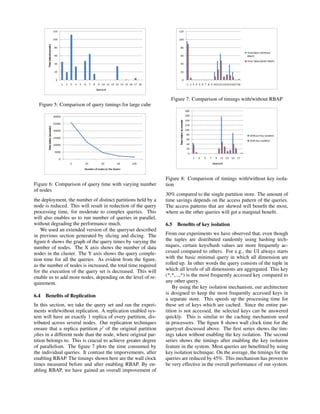
Table 1: Base table AdImpressions for a data warehouse
tain this fluidity of resources, we have had to reinvent our
approach to materialization, optimization and manageabil-
ity. We achieve materialization performance by allocating
scores of nodes for a short period of time. In query opti-
mization, our focus is on building new copies of data that
can be exploited for parallelism. For manageability, our
primary design goal is to identify the data value combina-
tion that are slowing down the queries so that when nodes
are added, load balancing of the partition housing these
combination can happen appropriately.
Specifically, we will describe 3 innovations in the area
of processing multi-dimensional data on the cloud:-
1) Partition Management for Low Cost. On the cloud,
nodes can be added and removed within minutes. We found
that node addition or removal needs to go hand-in-hand
with optimal redistribution of data. Blindly adding par-
titions or clones of partitions without taking into account
query performance would mean little or no benefit with
node addition. The partition manager in JovianDATA cre-
ates different tiers of partitions which may or may not be
attached to an active computing resource.
2) Replication to improve Query Performance. In a
cloud computing environment, resources should be added
to fix specific problems. Our system continuously monitors
the partitions that are degrading query performance. Such
partitions are automatically replicated for higher degree of
parallelism.
3) Materialization with Intermittent Scalability. We ex-
ploit the cloud’s ability to provision hundreds of nodes
to materialize the most expensive portions of a multi-
dimensional cube using an inordinately high number of
computing nodes. If a specific portion of data (key) is sus-
pected in query slowdown, we dynamically provision new
resources for that key and pre-materialize some query re-
sults for that key.
2 Representing and Querying Multidimen-
sional Data
The query language used in our system is the MDX lan-
guage. MDX and XMLA (XML for Analysis) are the well
known standards for querying and sending the multidimen-
sional data. For more details about MDX, please refer to
[12]. During the execution of an MDX query in the sys-
tem, the query processor may need to make several calls
to the underlying store to retrieve the data from the ware-
house. Design and complexity of the data structures which
carries this information from query processor to the store is
crucial to the overall efficiency of the system.
We use a proprietary tuple set model for accessing the
multidimensional data from the store. The query processor
Figure 1: Dimensions in the simple fact table
sends one or more query tuples and receives one or more
intersections in the form of result tuples. For illustration
purposes, we use the following simple cube schema from
the table 1.
Example: In an online advertising firm’s data ware-
house, Data are collected under the scheme AdImpres-
sions(Country, State, City, Year, Month, Day, Impression).
The base table which holds the impression records is shown
in table 1. Each row in the table signifies the number
of impression of a particular advertisement recorded in a
given geographical region at a given date. The column Im-
pression denotes the number of impressions recorded for
a given combination of date and region. This table is also
called as the fact table in data warehousing terminology.
The cube AdImpressions has two dimensions: Geogra-
phy, Time. The dimensions and the hierarchy are shown in
the figure 1. Geography dimension has three levels: coun-
try, state and city. Time dimension has three levels: year,
month and day. We have one measure in the cube called
impressions. We refer to this cube schema throughout this
paper to explain various concepts.
2.1 Tuple representation
The object model of our system is based on the data struc-
ture, we call as ‘tuple’. This is similar to the tuple used in
MDX notation, with a few proprietary extensions and en-
hancements. A tuple consists of set of dimensions and for
each dimension, it contains the list of levels. Each level
contains one of the 3 following values. 1) An ‘ALL’, indi-
cating that this level has to be aggregated. 2).MEMBERS
value indicating all distinct values in this level 3) A string
value indicating a particular member of this level.
Our system contains a tuple API, which exposes sev-
eral functions for manipulating the tuples. These include
setting a value to level, setting a level value to aggregate,
Crossjoining with other tuples etc.
2.1.1 Basic Query
We will explain the tuple structure by taking an example of
a simple MDX query shown in query 1.
The query processor will generate the tupleset shown
below for evaluating query 1. Note that, the measures are
not mentioned explicitly, because in a single access we can
fetch all the measure values.
An <ALL> setting for a particular level indicates that
the corresponding level has to be aggregated. Even though
the query doesn’t explicitly mention about the aggregation

3. on these levels, it can be inferred from the query and the
default values of the dimensions.
SELECT
{[Measures].[Impressions]} ON COLUMNS
,{
(
[Geography].[All Geographys].[USA]
,[Time].[All Times].[2007]
)
} ON ROWS
FROM [Admpressions]
Query 1: Simple tuple query
Country State City Year Month Day
USA ALL ALL 2007 ALL ALL
Query tupleset for Query 1
2.1.2 Basic Children Query
Query 2 specifies that the MDX results should display
all the children for the state ‘CALIFORNIA’ of country
‘USA’, for the june 2007 time period on the rows. Ac-
cording to the dimensional hierarchy, this will show all the
cities of the state ‘CALIFORNIA’. The corresponding tu-
ple set representation is shown below.
SELECT
{[Measures].[Impressions]} ON COLUMNS
,{
(
[Geography].[All Geographys].[USA].[CALIFORNIA].children
,[Time].[All Times].[2007].[June]
)
} ON ROWS
FROM [AdImpressions]
Query 2: Query with children on Geography dimension
Country State City Year Month Day
USA CALIFORNIA .MEMBERS 2007 June ALL
Query tupleset for Query 2
As described above, .MEMBERS in the City level indi-
cates that all the distinct members of City level are needed
in the results. After processing this tuple set, the store will
return several multidimensional result tuples containing all
the states in the country ‘USA’.
2.1.3 Basic Descendants Query
Query 3 asks for all the Descendants of the country ‘USA’,
viz. all the states in the country ‘USA’ and all the cities of
the corresponding states.The corresponding tuple set repre-
sentation is shown below.
SELECT
{[Measures].[Impressions]} ON COLUMNS
,{
Descendants
(
[Geography].[All Geographys].[USA]
,[CITY]
,SELF AND BEFORE
)
} ON ROWS
FROM [AdImpressions]
Query 3: Query with descendants on Geography
dimension
Country State City Year Month Day
USA .MEMBERS ALL ALL ALL ALL
USA .MEMBERS .MEMBERS ALL ALL ALL
Query tupleset for Query 3
Descendants operator will be resolved by the compiler at
the compile time and will be converted to the above tuple
notation. The first tuple in the tuple set represents all the
states in the country ‘USA’. The second tuple represents all
the cities of all the states for the country ‘USA’.
We use several other complex notations, to represent
query tuples of greater complexity. E.g., queries that con-
tain MDX functions like Filter(), Generate() etc. In the in-
terest of the scope of this paper, those details are intention-
ally omitted.
3 Architecture
The figure 2 depicts the high level architecture of the Jo-
vianDATA MDX engine. In this section, we give a brief
introduction about the various components of the architec-
ture. More detailed discussion of individual components
will appear in subsequent sections.
Figure 2: JovianDATA high level architecture
The query processor of our system consists of parser,
query plan generator and query optimizer with a transfor-
mation framework. The parser accepts a textual represen-
tation of a query, transforms it into a parse tree, and then
passes the tree to the query plan generator. The transforma-
tion framework is rule-based. This module scans through
query tree and compresses the tree as needed, and converts
the portions of tree to internal tuple representation and pro-
prietary operators. After the transformation, a new query
tree is generated. A query plan is generated from this trans-
formed query tree. The query processor executes the query
according to the compressed plan. During the lifetime of
a query, query process may need to send multiple tuple re-
quests to the access layer.
The tuple access API, access protocols, storage module
and the metadata manager constitutes the access layer of
our system. The query processor uses the tupleset notation
described in the previous section, to communicate with the
access layer. The access layer accepts a set of query tuples
and returns a set of result tuples. The result tuples typically
contain the individual intersections of different dimensions.
The access layer uses the access protocols to resolve the set

4. of tuples. It uses the assistance of metadata manager to re-
solve certain combinations. The access layer then instructs
the storage module to fetch the data from the underlying
partitions.
A typical deployment in our system consists of several
commodity nodes. Broadly these nodes can be classified
into one of the three categories.
Customer facing/User interface nodes: These nodes
will take the input from an MDX GUI front end. These
node hosts the web services through which user submits
the requests and receives the responses.
A Master node: This node accepts the incoming MDX
queries and responds with XMLA results for the given
MDX query.
Data nodes: There will be one or more data nodes in
the deployment. These nodes will host several partitions of
the data. These nodes typically wait for the command from
the storage module, processes them and returns the results
back.
4 Data Model
In this section we discuss the storage and data model of our
core engine. The basic component of the storage module in
our architecture is a partition. After building the data cube,
it is split into several partitions and stored in the cluster.
Every partition is hosted by one or more of the data nodes
of the system.
In a typical warehouse environment, the amount of data
accesses by the MDX query is small compared to the size
of the whole cube. By carefully exploiting this behavior,
we can achieve the desired performance by intelligently
partitioning the data across several nodes. Our partition
techniques are dictated by the query behavior and the cloud
computing environment.
In order to distribute the cube into shared nothing parti-
tions, we have several choices with respect to the granular-
ity of the data.
The three approaches[6] that are widely used are,
• Fact Table: Store the data in a denormalized fact
table[10]. Using the classic star schema methodology,
all multi-dimensional queries will run a join across the
required dimensional table.
• Fully Materialized: Compute the entire cube and
stored in a shared nothing manner. Even though com-
puting the cube might be feasible using hundreds of
nodes in the cloud, the storage costs will be prohibitive
based on the size of the fully materialized cube.
• Materialized Views: Create materialized views using
cost or usage as a metric for view selection[9]. Ma-
terialized views are query dependent and hence can-
not become a generic solution without administrative
overhead.
Country State City YearMonthDayImpressions
USA CALIFORNIASAN FRANCISCO2009 JAN 12 43
USA TEXAS HOUSTON 2009 JUN 3 33
Table 2: Sample fact table
The JovianDATA system takes the approach of materi-
alized tuples rather than materialized views. In the next
section, we describe the storage module of our system. For
illustration purposes, we assume the following input data
of the fact table as defined in table 2. We use query 1 and 2
from the section 2 for evaluating our model.
Functionally, our store consists of dimensions. Dimen-
sions consist of levels arranged in a pre-defined hierarchi-
cal ordering. Figure 1 show examples of the ‘GEOGRA-
PHY’ and ‘TIME’ dimensions. A special dimension called
‘MEASURES’ contains levels that are not ordered in any
form. An example level value within the ‘MEASURES’
dimension is ‘IMPRESSIONS’. Level values within the
‘MEASURES’ dimension can be aggregated across rows
using a predefined formula. For the ‘IMPRESSIONS’ mea-
sure level, this formula is simple addition.
Among all the columns in fact table, only selected sub-
set of columns are aggregated. The motive behind the par-
tial aggregated columns will be elaborated more in further
sections. This set of dimension levels, which are to be ag-
gregated are called Expensive levels and the others as cheap
(or non-expensive) levels. When choosing levels that are to
be aggregated, our system looks at the distribution of data
in the system, and does not bring in explicit assumptions
about aggregations that will be asked by queries executing
on the system. Competing systems will choose partially
aggregated levels based on expected incoming queries - we
find that these systems are hard to maintain if query pat-
terns change, whereas our data based approach with hash
partitioning leads to consistently good performance on all
queries.
For illustrative purposes, consider ‘YEAR’ and
‘STATE’ as aggregation levels for the following 9 in-
put lines. If incoming rows are in the form of (YEAR,
MONTH, COUNTRY, STATE, IMPRESSIONS) as shown
in table 3 then the correponding table after partial aggreag-
tion is as shown in table 4.
Year Month Country State Impressions
2007 JAN USA CALIFORNIA 3
2007 JAN USA CALIFORNIA 1
2007 JAN USA CALIFORNIA 1
2007 JAN USA CALIFORNIA 1
2007 JAN USA CALIFORNIA 1
2007 FEB USA TEXAS 10
2007 FEB USA TEXAS 1
2007 FEB USA TEXAS 1
2007 FEB USA TEXAS 1
Table 3: Pre-aggregated Fact Table
Note that we have aggregated dimension-levels that we
deem to be expensive and not aggregated other dimension
levels.
In many cases, for terabytes of data, we observed that
the size of the partially aggregated cube ends up being
smaller than the size of the input data itself.

5. Year Month Country State Impressions
2007 JAN USA CALIFORNIA 7
2007 FEB USA TEXAS 13
ALL JAN USA CALIFORNIA 7
ALL FEB USA TEXAS 13
ALL JAN USA ALL 7
ALL FEB USA ALL 13
2007 JAN USA ALL 7
2007 FEB USA ALL 13
Table 4: Partially-aggregated Cube
4.1 Cheap dimensions storage model
Cheap dimension levels helps in compressing the cube in
two ways. Firstly, by not aggregating these levels, multi-
ple aggregation combinations will be avoided, thus keep-
ing the cube size low. Secondly, since these levels are
not aggregated, for every combination of expensive dimen-
sions, the slow dimension combinations are limited, but
repeated. This redundancy in the slow dimension combi-
nations can be exploited by isolating the slow dimension
combinations into a separate table, and using the identi-
fiers to re-construct the original rows. In this technique, we
split the cube data vertically, and create an identifier table
or what we call cheap dimension table. Thus for the cube
shown in table 4 the cube and the cheap dimension table
formed after vertical decomposition are shown in table 5
and table 6 respectively.
Year State CheapDimId Impressions
2007 CALIFORNIA ID 1 7
2007 TEXAS ID 2 13
ALL CALIFORNIA ID 1 7
ALL TEXAS ID 2 13
ALL ALL ID 1 7
ALL ALL ID 2 13
2007 ALL ID 1 7
2007 ALL ID 2 13
Table 5: Partially-aggregated Cube with CheapDimId
CheapDimId Month Country
ID 1 JAN USA
ID 2 FEB USA
Table 6: Cheap Dimension Table
4.2 Selecting Expensive dimension levels
Partial aggregation plays key role in our cube subsystem.
Out of n columns in the fact table, m columns will be
marked as expensive columns. Remaining (n-m) columns
will be marked as non-expensive. The division is based on
the empirical observation of the time bounds of different set
of configurations and following factors. The storage model
for expensive and non-expensive dimension is motivated to
provide the faster response times for expensive keys in the
tuple. The partition table is partitioned vertically, using ex-
pensive and non-expensive columns. The row relationships
are maintained by encoding each slow dimension level’s
unique combination. This storage structure, along with the
aggregation scheme influences the choice of expensive di-
mensions and non-expensive dimensions. The following
are some of the key factors which affect the choice. The
user query contains either ‘*’ or ‘value’ in each of the ag-
gregate levels.
• Cheap (Slow) Dimension Statistics:
– Distinct value: Queries which involves Distinct
value in the children query involves selecting
one row from the slow dimension table
– Aggregate Value: Queries which involves ag-
gregate in children levels, needs to perform ag-
gregation on the entire slow dimension table in
worst case.
• Expensive (Fast) (Dim)ension Statistics
– Expensive (Fast) Dim combination size : For
certain combinations of the expensive dimen-
sions, the selectivities of the slow dimension
combinations are lower, which leads to process-
ing of more rows.
– Expensive (Fast) Dim per-partition Key cardi-
nality: This involves how many keys are packed
in a single partition or single node. As more keys
are packed in a single node, the access time in-
creases.
– Expensive (Fast) Dim Avg per-key size:
We use the following criteria to bifurcate the dimension
set into expensive and non expensive dimensions.
1. Cube compression: If the number of distinct values in
a dimension is small, the number of different combi-
nation it produces is much smaller. This results in a
compact cube.
2. Cube explosion: If there are multiple dimensions
listed as expensive, some dimensions are more likely
to produce exponential set of cube rows. This is called
as expression selectivity, and is a key factor in deter-
mining the expensive dimensions.
3. Slow dimension table size: Since the slow dimensions
are maintained in a separate table, as the more number
of slow dimensions participate, The size of this table
grows.
Once we have partially materialized the tuples, we par-
tition them using the expensive dimensions as the keys for
partitioning. In the next section, we show how these parti-
tions are managed.
4.3 Partition Manager
The JovianDATA storage system manages its partitions
across different tiers of storage. The storage tiers are used
to maintain the Service Level Agreements at a per partition
level and also to achieve the desired performance levels.
The outline of the storage system is shown in the figure 3.
There are 5 different states for an individual partition

6. Figure 3: Partition states in the storage
• Archived: A partition is in the Archived state when
the data is stored in a medium that cannot be used to
resolve queries. In other words, the data in archived
partitions is not immediately accessible for querying.
To make an archived partition available for queries or
updates, the archived partition has to be promoted to
the operational state. In the figure above, the parti-
tion P3 is in archived stage. A partition is moved
to the archival stage if the partition manager detects
that partition is not being used for queries or updates.
Of course, there is a cost to bringing a partition to
‘life’. The challenge is to identify the partitions that
are needed in archival storage. In Amazon Web Ser-
vices, the archival storage is the S3 buckets. Every
partition is stored as an S3 bucket.
• Operational: A partition is in the Operational state
when the partition’s data can be used for resolution of
a tuple. All tuple resolution occurs on the CPU of the
node which owns the partition. The operational state
is the minimum state for a partition to be usable in a
query. A partition in operational state cannot be used
for updates. A partition in operational state can be
promoted to the load state or to the replication state.
In the figure above, the partitions P1 and P2 are in
the operational state. These partitions can be used to
directly resolve tuples for incoming queries. In Ama-
zon Web Services, the operational partition’s owner is
an EC2 compute node. An EC2 node is a virtual ma-
chine with a disk attached to it. When query comes in
and a tuple is located on an operational partition, any
late aggregations are performed on the EC2 node that
owns the partition.
• Load: A partition is in the Load state when the par-
tition’s data can be used for incremental updates or
for a ‘first time’ load. No tuples can be resolved on
these systems. A partition in the load state can be
transitioned to archive storage before it can become
operational. In Amazon Web Services, a partition in a
load state is generally represented by a temporary EC2
compute node. Temporary EC2 nodes are deployed to
generate cube lattices or update existing lattices of the
cube.
• Replicate: A partition is in the replicate state when
the partition’s data is hosted on multiple nodes. The
primary goal for partition to move into replicated state
is to improve parallelism of a single query. In the
figure above, the Partition P2 has been identified for
replication and is hosted on 5 different hosts. In Ama-
zon Web Services, a partition in replicated state exists
with different copies residing on different EC2 com-
pute nodes. Temporary EC2 nodes might be deployed
to host replicas of a partition.
• Isolated A partition is in the materialized state when
a partition’s keys have been isolated and fully materi-
alized. Partitions are moved into this state when the
‘last minute’ aggregations are taking too much time.
4.4 Cost Based Partition Management
The partition manager’s ability to divide partitions into
Archived, Operational, Load, Replicate and Isolate cat-
egories allows for a system which uniquely exploits the
cloud. Each state has a different cost profile
• Archived: An archived partition has almost zero cost
because it resides on a secondary storage mechanism
like S3 which is not charged by the hour. We try to
keep the least access partition in the archived state.
• Operational: Partitions in operational state are ex-
pensive because they are attached to actual nodes
which are being charged by the hour on the cloud plat-
form.
• Load: Partitions in load state are expensive for re-
ally short periods of time where tuple materialization
might require a high number of nodes.
• Replication: Partitions in Replication state are more
expensive than operational partitions as each replica
is hosted on a separate node. In the replicated access
protocol section, we explain the selection criteria for
moving a partition into the replicated state.
• Isolated: Isolated keys are the most expensive be-
cause they have dedicated hosts for single keys. In
Isolation Based Access Protocol (IBAP) section, we
explain the selection criteria for moving a key into an
isolated partition state.
The cloud environment presents the unique opportunity
to dynamically add or remove the nodes based on the num-
ber of partitions that are in various states. The cost of main-
taining a data processing system is the function over the
cost of each state multiplied by the number of partitions in
each state. When working with a large number of partitions

7. (more than 10,000), the cost of a system can be brought up
or down simply by moving a few partitions from one state
to another.
4.5 Distributing and querying data
We partition the input data based on a hash key calculated
on the expensive dimension level values. So, all rows with
a YEAR value of ‘2007’ and a STATE value of ‘TEXAS’
will reside in the same partition. Similarly, all rows with
(YEAR, STATE) set to (‘2007’, ALL) will reside in the
same partition. We will see how this helps the query sys-
tem below. Note that we are hashing on ‘ALL’ values also.
This is unlike existing database solutions[5] where hashing
happens on the level values in input data rows. We hash
on the level values in materialized data rows. This helps
us create a more uniform set of partitions. These partitions
are stored in a distributed manner across a large scale dis-
tributed cluster of nodes.
If the query tuple contains ‘*’ on the cheap dimension
levels, we need to perform an aggregation. However, that
aggregation is performed only on a small subset of the
data, and all of that data is contained within a single par-
tition. If multiple tuples are being requested, we can triv-
ially run these requests in parallel on our shared nothing
infrastructure, because individual tuple requests have no
inter-dependencies and only require a single partition to run
against.
5 Access protocols
An access protocol is a mechanism by which our system
resolves an incoming request in access layer. We have ob-
served that the response time of the access layer is greatly
improved by employing multiple techniques for different
type of incoming tuples. For e.g., tuples which require a lot
of computing resources are materialized during load time.
Some tuples are resolved through replicas while others are
resolved through special type of partitions which contain a
single, expensive key.
5.0.1 On Demand Access Protocol (ODAP)
We classify On Demand Access Protocols as multi-
dimensional tuple data structures that are created at run
time, based on queries, which are slowing down. Here,
the architecture is such that the access path structures are
not updated, recoverable or maintained by the load sub sys-
tem. In many cases, a ‘first’ query might be punished rather
than maintaining the data structures. The data structures
are created at query time after the compiler decides that the
queries will benefit from said data structures.
ODAP data structures are characterized by the low cost
of maintenance because they get immediately invalidated
by new data and are never backed up. There is a perceived
cost of rematerializing these data structures but these might
be outweighed by the cost of maintaining these data struc-
tures.
5.0.2 Load Time Access Protocol (LTAP)
We classify Load Time Access Protocols as multi-
dimensional tuple data structures that are created and main-
tained as a first class data object. The classical LTAP is
B-Tree data structure. Within this, we can classify these
as OLTP(OnLine Transaction Processing) data structures
and OLAP(OnLine Analytical Processing) data structures.
OLTP data structures heavy concurrency and granular up-
dates. OLAP data structures might be updated ’once-a-
day’.
LTAP data structures are characterized by the high cost
of maintenance because these data structures are usually
created, as a part of the load process. These structure also
need to be backed up (like any data rows),during backup
process. Any incremental load should either update/rebuild
these structures.
5.0.3 Replication Based Access Protocol (RBAP)
We have observed that the time required for data retrieval
for a given MDX query is dominated by the response time
of the largest partition the MDX query needs to accesses.
Also in Multi Processing environment the frequently used
partitions prove to be a bottle-neck with requests from mul-
tiple MDX queries being queued up at a single partition.To
reduce time spent on a partition, we simply replicate them.
The new replicas are moved to their own computing re-
sources or on nodes which have smaller partitions.
For eg. Partition which contains ‘ALL’ value in all the
expensive dimensions is the largest partition in a material-
ized cube. So any query which has the query tupleset con-
taining set of query tuples being resolved by this partition
will have a large response time due to this bottle neck parti-
tion. In absence of replicas all the query tuples needed to be
serviced by this partition line up on the single node which
has the copy of that partition. This leads to time require-
ment upperbounded by Number of Tuples * Max. Time for
single tuple scan.
However if we have replicas of the partition, we can split
the tuple set into smaller sub. sets and execute them in
parallel on different replicas. This enables the incoming
requests to be distributed across several nodes. This would
bring down the retrieval time atleast to Number of Tuples *
Max. Time for single tuple scan / Number of Replicas.
When we implement RBAP we have to answer ques-
tion like, ”How many partitions to replicate?”. If we repli-
cate less number of partitions we are restricting the class of
queries which will be benefitted from the new access proto-
col. Replicating all the data is also not feasible. Also while
replicating we have to maintain the load across the nodes
and make sure that no nodes get punished in the process of
replication.
Conventional data warehouses generally use replication
for availability. Newer implementations of big data pro-
cessing apply the same replication factor across the entire
file system. We use automatic replication to improve query
performance.
The RBAP protocol works as follows:

8. 1. After receiving the query tuples, group the tuples
based on their HashValue.
2. Based on HashValue to Partition mapping, enumerate
the partition that can resolve these tuples.
3. For each partition, enumerate the hosts which can ac-
cess this partition. If the partition is replicated, the
system has to choose the hosts which should be ac-
cessed to resolve the HashValue group.
4. We split the tuple list belonging to this HashValue
group, uniformly across all these hosts, there by di-
viding the load across multiple nodes.
5. Each replica thus shares equal amount of work. By
enabling RBAP for a partition, all replica nodes can
be utilized to answer a particular tuple set.
By following RBAP, we can ideally get performance im-
provement by a factor which is equal to the number of repli-
cas present. Empirically we have observed a 3X improve-
ment in execution times on a 5 node cluster with 10 largest
partitions being replicated 5 times.
We determine the number of partitions to replicate by lo-
cating the knee of the curve formed by plotting the partition
sizes in decreasing order. To find the knee we use the con-
cept of minimum Radius of Curvature (R.O.C.)as described
by Weisstein in [16]. We pick the point where the R.O.C. is
minimum as the knee point and the corresponding x-value
as the number of partitions to be replicated. The formulae
for R.O.C. we used is R.O.C. = y /(1 + (y )2
)1.5
Example:
Consider the MDX query 4 and its query tuple set
SELECT
{[Measures].[Impressions]} ON COLUMNS
,{
,[Time].[All Times].[2008].Children
} ON ROWS
FROM [Admpressions]
WHERE [Geography].[All Geographys].[USA].[California]
Query 4: Query with children on Time dimension
TupleID Year Month Country State
T1 2008 1 United States California
T2 2008 2 United States California
T3 2008 3 United States California
T4 2008 4 United States California
T5 2008 5 United States California
T6 2008 6 United States California
T7 2008 7 United States California
T8 2008 8 United States California
T9 2008 9 United States California
T10 2008 10 United States California
T11 2008 11 United States California
T12 2008 12 United States California
Query tupleset for Query 4
All the query tuples from the above tupleset have the
same expensive dimension combination of year = 2008 ;
state = California. This implies a single partition services
all the query tuples. Say the corresponding partition which
hosts the data corresponding to fast dimension year = 2008
; state = California is Partition P9986 and in absence of
replicas, let the lone copy be present on host H1. In this
scenario all the 12 query tuples will line up at H1 to get the
required data. Consider a scan required to a single query
tuple require maximum time t1 secs. Now H1 services each
query tuple in a serial manner. So the time required for it
to do so is bounded by t1 * 12.
Now let us consider RBAP in action. First we will repli-
cate the partition P9986 on multiple hosts say H2, H3 and
H4. Now partition P9986 has replicas on H1, H2, H3 and
H4. Let a replica of Partition Pj on host Hi be indicated
by the pair (Pj, Hi). Once the query tupleset is grouped
by their Expensive Dimension combination the engine re-
alises that the above 12 query tuples belong to the same
group. After an Expensive Dimension - Partition look up
the engine determines that this group of query tuple can
be serviced by partition P9986. A further Partition-Host
look up determines that P9986 resides on H1, H2, H3 and
H4. Multiple query tuples in the group and multiple repli-
cas of the corresponding partition, make this group eligible
for RBAP. So the scheduler now divides the query tuples
amongst the replicas present. So T1, T5 and T9 are serviced
by (P9986,H1), T2, T6 and T10 are serviced by (P9986,H2),
T3, T7 and T11 are serviced by (P9986,H3) and T4, T8 and
T12 are serviced by (P9986,H4). Due to this access path
we now bounded the time required to retrieve the required
data to t1 * 3. So by following RBAP, we can ideally get
performance improvement by a factor which is equal to the
number of replicas present.
A crucial problem which needs to be answered while
replicating partitions is , ‘Which partitions to replicate?’.
An unduly quick decision would declare that partition as
the size metric. The greater the size of the partition, the
greater its chances of being a bottleneck partition. But this
conception is not true, since a partition containing 5000 Ex-
pensive Dimensions (ED) combinations each contributing
to 10 rows in the partition will require lesser response time
than a partition containing 5 ED combinations with each
expensive dimension tuple contributing to 10000 rows. So
the problem drills down to identifying partitions contain-
ing ED combination which lead to the bottle neck. Let
us term such ED combinations as hot-keys. Apart from
the knee function described above, we identify the tuples
that contribute to the final result for frequent queries. Take
for example a customer scenario where the queries were
sliced upon the popular states of New York, California and
Florida. These individual queries worked fine, but queries
with [United States].children took considerable more time
than expected. On detail analysis of the hot-keys we re-
alised that the top ten bottle neck keys were
No. CRCVALUE SITE SECTION DAY COUNTRY NAME STATE DMA
1 3203797998 * * * * *
2 1898291741 * * 256 * *
3 1585743898 * * 256 * 13
4 2063595533 * * * * 13
5 2116561249 NO DATA * * * *
6 187842549 NO DATA * 256 * *
7 7291686 * * * VA *
8 605303601 * * 256 VA *
9 83518864 * * 256 MD *
10 545330567 * * * MD *
Top ten bottle-neck partitions
Before running the hot key analysis, we were expecting
ED combinations 1, 2, 3, 4, 5, 6 to show up. But ED com-

9. bination 7, 8, 9,10 provided great insights to the customer.
It shows a lot of traffic being generated from the state of
VA and MD. So after replicating the partitions which con-
tain these hot keys and then enabling RBAP we achieved a
3 times performance gain.
The next question we must answer is, ‘Does RBAP help
every-time?’ The answer to this question is - No, RBAP
deteriorates performance in the case where the serial exe-
cution is lesser than parallelization overhead. Consider a
low cardinality query which would be similar to Query 4
but choose a geographical region other than USA, Calfor-
nia, eg. Afganistan.
Suppose this query returns just 2 rows. then it does not
make sense to distribute the data retrieval process for this
query.
So to follow RBAP the query tuple set must satisfy the
following requirements 1) The query tuple set must consist
of multiple query tuples having the same ED combination
and hence targeting the same partition. 2) The partition
which is targeted by the query tuples must be replicated on
multiple hosts. 3) The ED targeted must be a hot key.
5.0.4 Isolation Based Access Protocol (IBAP)
In cases where replication does not help, we found that the
system is serialized on a single key within the system. A
single key might be used to satisfy multiple tuples. For
such cases, we simply move the key into its own single key
partition. The single key partition is then moved to its own
host. This isolation helps tuple resolution to be executed on
its own computing resources without blocking other tuple
access.
6 Performance
In this section we start with evaluating the performance of
different access layer steps. We then evaluate the perfor-
mance of our system against a customer query load. We
are not aware of any commercial implementations of MDX
engines which handles 1 TB of cube data hence we are not
able to contrast our results with other approaches. For eval-
uating this query load, we use two datasets; a small data set
and a large data set. The sizes of the small cube and large
cube are 106 MB and 1.1 TB respectively. The configu-
ration of the two different cubes we use, are described in
table 7. The configuration of the data node is as follows.
Every node has 1.7 GB of memory, 160 GB of local in-
stance storage running on 32-bit platform having a CPU
capacity equivalent to 1.2 GHz 2007 Opteron.
6.1 Cost of the cluster
The right choice of the expensive and cheap levels, depends
on the cost of the queries in each of the models. Select-
ing the right set of expensive dimensions is equivalent to
choosing the optimum set of Materialize Views which is
know to be a NP hard problem[11], hence we use empir-
ical observations and data distribution statistics and set of
heuristics to determine the set of expensive dimensions.
The cloud system we use offers different types of com-
modity machines for allocation. In this section, we will
explain the dollar cost of executing a query in the cluster
with and without our architecture. The cost of each of these
nodes with different configurations is shown in table 8.
Metric small cube large cube
Number of rows in input data 10,000 1,274,787,409
Input data size (in MB) 6.13 818,440
Number of rows in cube 454,877 4,387,906,870
Cube size (in MB) 106.7 1,145,320
Number of dimensions 16 16
Total levels in the fact table 44 44
Number of expensive levels 11 11
Number of partitions 30 5000
Number of data nodes in the deployment 2 20
Table 7: Data sizes used in performance evaluation
Cost of the cluster ($s per day)
Number of
data nodes
High Memory instances High CPU Instances
XL XXL XXXXL M XL
5 60 144 288 20.4 81.6
10 120 288 576 40.8 163.2
20 240 576 1152 81.6 326.4
50 600 1440 2880 204 816
100 1200 2880 5760 408 1632
Table 8: Cluster costs with different configurations
The high memory instances have 160GB, 850GB, 1690
GB of storage respectively. Clusters which hold cubes of
bigger sizes need to go for high memory instances. The
types of instances we plan to use in the cluster may also
influence the choice of expensive and cheap dimensions.
In this section we contrast our approach with the Rela-
tional Group By approach. We use the above cost model to
evaluate the total cost of the two approaches. Let us con-
sider query 5 on the above mentioned schema and evaluate
the cost requirement of both the model.
SELECT
{
[Measures].[Paid Impressions]
} ON COLUMNS
,Hierarchize
(
[Geography].[All Geographys]
) ON ROWS
FROM [Engagement Cube]
Query 5: Query with Hierarchize operator
Firstly we evaluate the cost for our model, then for the
relational Group-by model[1] followed by a comparision
of the two. We took a very liberal approach in evaluat-
ing the performance of SQL approach. We assumed the
data size, which can result after applying suitable encoding
techniques. We created all the necessary indices, and made
sure all the optimizations are in place.
The cost of the query 5 is 40 seconds in the 5-node system with high memory
instances.
The cost of such a cluster is 144$ per day, for the 5 nodes.
During load time we use 100 extra nodes, which will live upto 6 hours. Thus the
temporary resources accounts to 720$.
If the cluster is up and running for a single day the cost of the cluster is 864$ per
day.
For 2,3,5,10 and 30 days the cost of the deployment will be 504, 384, 288, 216,
168$ per day respectively.

10. Cost for JovianDATA model of query 5
Let us assume a naive system with no materialized views. This system has the raw
data partitioned into 5000 tables. Each node will host as many partitions as allowed
by the storage.
The cost for individual group by query is on a partition is 4 sec.
To achieve the desired 40 seconds, number of partitions node can host are 40/4 =10
Number of nodes required = 5000/10 = 500
Cost of the cluster(assuming low memory instances) = 500*12 = 6000$.
Cost for Relational World model of query 5
The ratio of the relational approach to our approach is 6000/144 = 41:1
Assuming the very best of a materialized view, in which we need to process only
25% of the data,
The cost of the cluster is 6000/4 = 1500$, which is still 10 times more than our
approach.
JovianDATA Vs. Relational Model cost comparision for
Query 5
Similar comparision was done for query 6 which costs
27s in our system.
SELECT
{
Measures.[Paid Impressions]
} ON COLUMNS
,Hierarchize
(
[Geography].[All Geographys].[United States]
) ON ROWS
FROM [Engagement Cube]
Query 6: Country level Hierarchize query
The average cost for individual group by query is on a partition is 1.5 sec (after
creating the necessary indices and optimizations).
For 27 secs, number of partitions node can host are 27/1.5 =18
Number of nodes required = 5000/18 = 278
Cost of the cluster(with low memory instances) = 278*12 = 3336$.
The ratio of relational approach to our approach is 3336/144 = 23:1
Assuming a materialized view, which needs only 25% of the data, The cost of the
cluster is 3336/4 = 834$, which is still 6 times more than our approach.
JovianDATA Vs. Relational Model cost comparision for
Query 6
6.2 Query performance
In this section, we evaluate the end-to-end performance
of our system on a real world query load. The customer
query load we use, consists of 18 different MDX queries.
The complexity of the queries varies from moderate to
heavy calculations involving Filter(), Sum(), Topcount()
etc. Some of the queries involves calculated members,
which performs complex operations like Crossjoin(), Fil-
ter() and Sum() on the context tuple.
The structure of those queries are shown in table 9. We
have run these queries against the two cubes described in
previous section.
The figure 4 shows the query completion times for the
18 queries against the small cube. The timings for the large
cube are shown in figure 5. The X-axis shows the query id
and the Y-axis shows the wall clock time for completing the
query, in seconds. Each query involves several access layer
calls throughout the execution. The time taken for a query
depends on the complexity of the query and the number of
separate access layer calls it needs to make.
As evident from the figures, the average query response
time for the small cube is 2 seconds. The average query
response time for the large cube is 20 seconds. Our sys-
tem scales linearly even though the data has increased by
Query Number
of cal-
culated
measures
Number of inter-
sections for small
cube
Number of inter-
sections for large
cube
1 3 231 231
2 47 3619 3619
3 1 77 77
4 1 77 77
5 1 77 77
6 1 77 77
7 243 243 243
8 27 81 108
9 5 5 5
10 5 5 5
11 5 5 5
12 5 5 5
13 5 290 300
14 5 15 15
15 5 160 1370
16 4 12 12
17 4 4 4
18 4 4 4
Table 9: Queryset used in performance evaluation
Figure 4: Comparison of query timings for small cube
10,000 folds. The fact that the most of the queries are an-
swered in sub-minute time frame for the large cube, is an
important factor in assessing the scalability of our system.
Note that, the number of intersections in the large
dataset is higher for certain queries, when compared to that
of smaller dataset. Query 15 is one such query where the
number of intersections in large dataset is 1370, compared
to 160 of the small dataset. Even though the number of
intersections is more and the amount of data that needs
to be processed is more, the response time is almost the
same in both the cases. The distribution of the data across
several nodes and computation of the result in a shared-
nothing manner are the most important factors in achieving
this. To an extent, we can observe the variance in the query
response times, by varying the number of nodes. We will
explore this in the next section.
6.3 Dynamic Provisioning
As described in previous sections, every data node hosts
one or more partitions. Our architecture stores equal num-
ber of partitions in each of the data nodes. The distribution
of the partitions a tupleset will access is fairly random. If
two tuples can be answered by two partitions belonging to
the same node, they are scheduled sequentially for the com-
pletion. Hence by increasing the number of data nodes in

11. Figure 5: Comparison of query timings for large cube
Figure 6: Comparison of query time with varying number
of nodes
the deployment, the number of distinct partitions held by a
node is reduced. This will result in reduction of the query
processing time, for moderate to complex queries. This
will also enables us to run number of queries in parallel,
without degrading the performance much.
We used an extended version of the queryset described
in previous section generated by slicing and dicing. The
figure 6 shows the graph of the query times by varying the
number of nodes. The X axis shows the number of data
nodes in the cluster. The Y axis shows the query comple-
tion time for all the queries. As evident from the figure,
as the number of nodes is increased, the total time required
for the execution of the query set is decreased. This will
enable us to add more nodes, depending on the level of re-
quirement.
6.4 Benefits of Replication
In this section, we take the query set and ran the experi-
ments with/without replication. A replication enabled sys-
tem will have an exactly 1 replica of every partition, dis-
tributed across several nodes. Our replication techniques
ensure that a replica partition p of the original partition
plies in a different node than the node, where original par-
tition belongs to. This is crucial to achieve greater degree
of parallelism. The figure 7 plots the time consumed by
the individual queries. It contrast the imporvements, after
enabling RBAP. The timings shown here are the wall clock
times measured before and after enabling RBAP. By en-
abling RBAP, we have gained an overall improvement of
Figure 7: Comparison of timings with/without RBAP
Figure 8: Comparison of timings with/without key isola-
tion
30% compared to the single partition store. The amount of
time savings depends on the access pattern of the queries.
The access patterns that are skewed will benefit the most,
where as the other queries will get a marginal benefit.
6.5 Benefits of key isolation
From our experiments we have observed that, even though
the tuples are distributed randomly using hashing tech-
niques, certain keys/hash values are more frequently ac-
cessed compared to others. For e.g., the UI always starts
with the basic minimal query in which all dimension are
rolled up. In other words the query consists of the tuple in
which all levels of all dimensions are aggregated. This key
(*,*,...,*) is the most frequently accessed key compared to
any other query.
By using the key isolation mechanism, our architecture
is designed to keep the most frequently accessed keys in
a separate store. This speeds up the processing time for
these set of keys which are cached. Since the entire par-
tition is not accessed, the selected keys can be answered
quickly. This is similar to the caching mechanism used
in processors. The figure 8 shows wall clock time for the
queryset discussed above. The first series shows the tim-
ings taken without enabling the key isolation. The second
series shows the timings after enabling the key isolation
feature in the system. Most queries are benefitted by using
key isolation technique. On the average, the timings for the
queries are reduced by 45%. This mechanism has proven to
be very effective in the overall performance of our system.

12. 7 Conclusions and future work
In this paper, we have presented a novel approach of main-
taining and querying the data warehouses on cloud com-
puting environment. We presented a mechanism to com-
pute the combinations and distribute the data in an easily
accessible manner. The architecture of our system is suit-
able for data ranging from smaller data sizes to very large
data sizes.
Our recent development work is focused on several as-
pects in improving the overall experience of the entire de-
ployment. We will explain some of the key concepts here.
Each data node in our system will host several partitions.
We are creating replications of the partitions across differ-
ent nodes. i.e., a partition is replicated at a different node.
For a given tuple, the storage module, will pick up the least
busy node which is holding the partition. This will increase
the overall utilization of the nodes. The replication will
serve two different purposes of reducing the response time
of a query and increase the availability of the system.
Data centers usually offers high available disk space and
can serve as back up medium for thousands of terabytes.
When a cluster is not being used by the system, the entire
cluster along with the customer data can be taken offline
to a backup location. The cluster again can be restored by
using the backup disks whenever needed. This is an impor-
tant feature from the customer’s perspective, as the cluster
need not be running 24X7. Currently the cluster restore
time is varying from less than an hour to a couple of hours.
We are working on techniques which enable to restore the
cluster in sub hour time frame.
8 Acknowledgments
The authors would like to thank Prof. Jayant Haritsa, of In-
dian Institute of Science, Bangalore, for his valuable com-
ments and suggestions during the course of developing the
JovianDATA MDX engine. We would like to thank our
customers for providing us data and complex use cases to
test the performance of the JovianDATA system.
References
[1] R. Ahmed, A. Lee, A. Witkowski, D. Das, H. Su,
M. Zait, and T. Cruanes. Cost-based query transfor-
mation in oracle. In 32nd international conference on
Very Large Data Bases, 2006.
[2] I. Andrews. Greenplum database:critical mass inno-
vation. In Architecture White Paper, June 2010.
[3] N. Cary. Sas 9.3 olap server mdx guide. In SAS Doc-
umentation, 2011.
[4] R. Chaiken, B. Jenkins, P. ke Larson, B. Ramsey,
D. Shakib, S. Weaver, and J. Zhou. Scope: Easy
and efficient parallel processing of massive data sets.
In 34th international conference on Very Large Data
Bases, August 2008.
[5] D. Chatziantoniou and K. A. Ross. Partitioned opti-
mization of complex queries. In Information systems,
2007.
[6] S. Chaudhuri and U. Dayal. An overview of data
warehousing and olap technology. ACM SIGMOD
Record, 26(1):65–74, March 1997.
[7] D. Dibbets, J. McHugh, and M. Michalewicz. Oracle
real application clusters in oracle vm environments.
In An Oracle Technical White Paper, June 2010.
[8] EMC2. Aster data solution overview. In AsterData,
August 2010.
[9] L. Fu and J. Hammer. Cubist: a new algorithm for
improving the performance of ad-hoc olap queries. In
3rd ACM international workshop on Data warehous-
ing and OLAP, 2000.
[10] H. Gupta, V. Harinarayan, A. Rajaraman, and J. D.
Ullman. Index selection for olap. In Thirteenth Inter-
national Conference on Data Engineering, 1997.
[11] H. Gupta and I. S. Mumick. Selection of views to ma-
terialize under a maintenance cost constraint. pages
453–470, 1999.
[12] http://msdn.microsoft.com/en-
us/library/ms145595.aspx. MDX Language Ref-
erence, SQL Server Documentation.
[13] D. V. Michael Schrader and M. Nader. Oracle Ess-
base and Oracle OLAP. McGraw-Hill Osborne Me-
dia, 1 edition, 2009.
[14] J. Rubin. Ibm db2 universal database and the architec-
tural imperatives for data warehousing. In Informa-
tion integration software solutions White Paper, May
2004.
[15] M. Schrader. Understanding an olap solution from
oracle. In An Oracle White Paper, April 2008.
[16] E. W. Weisstein. Curvature. From MathWorld–A Wol-
fram Web Resource.