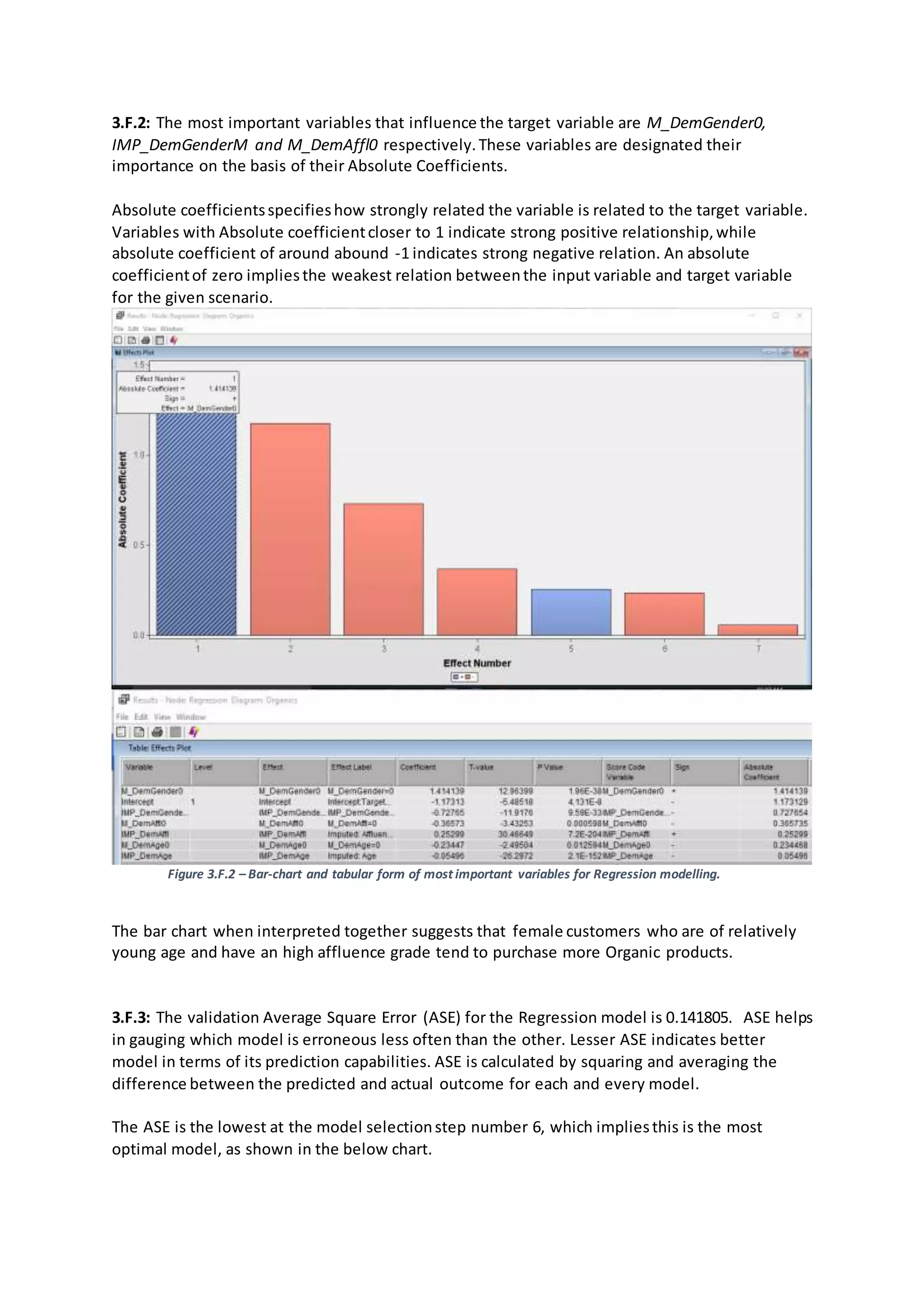
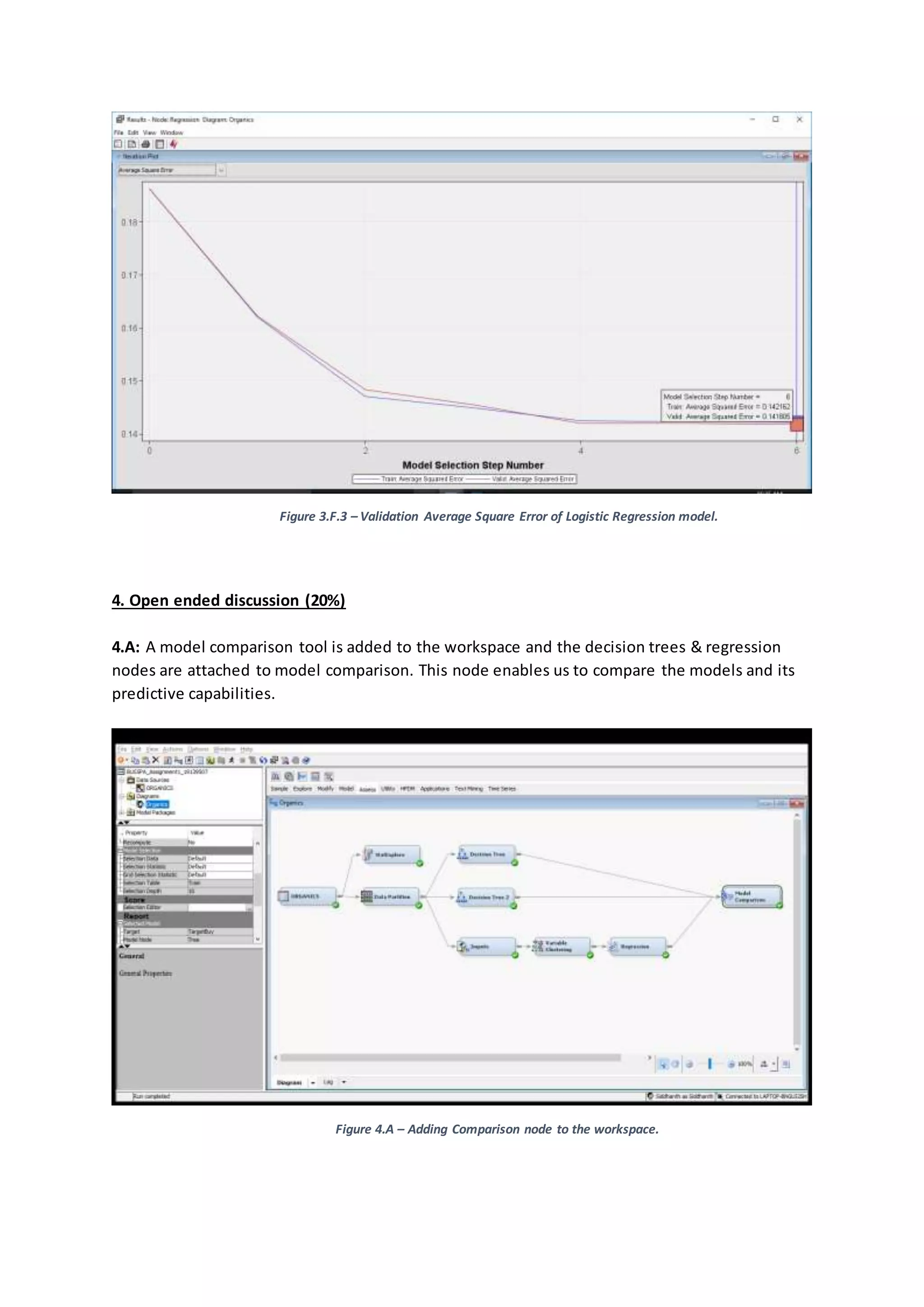
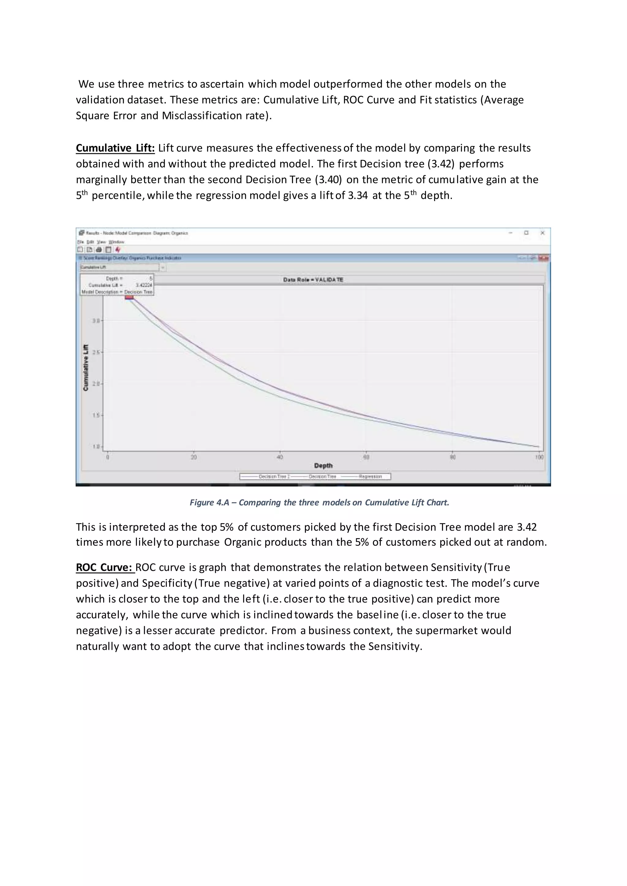
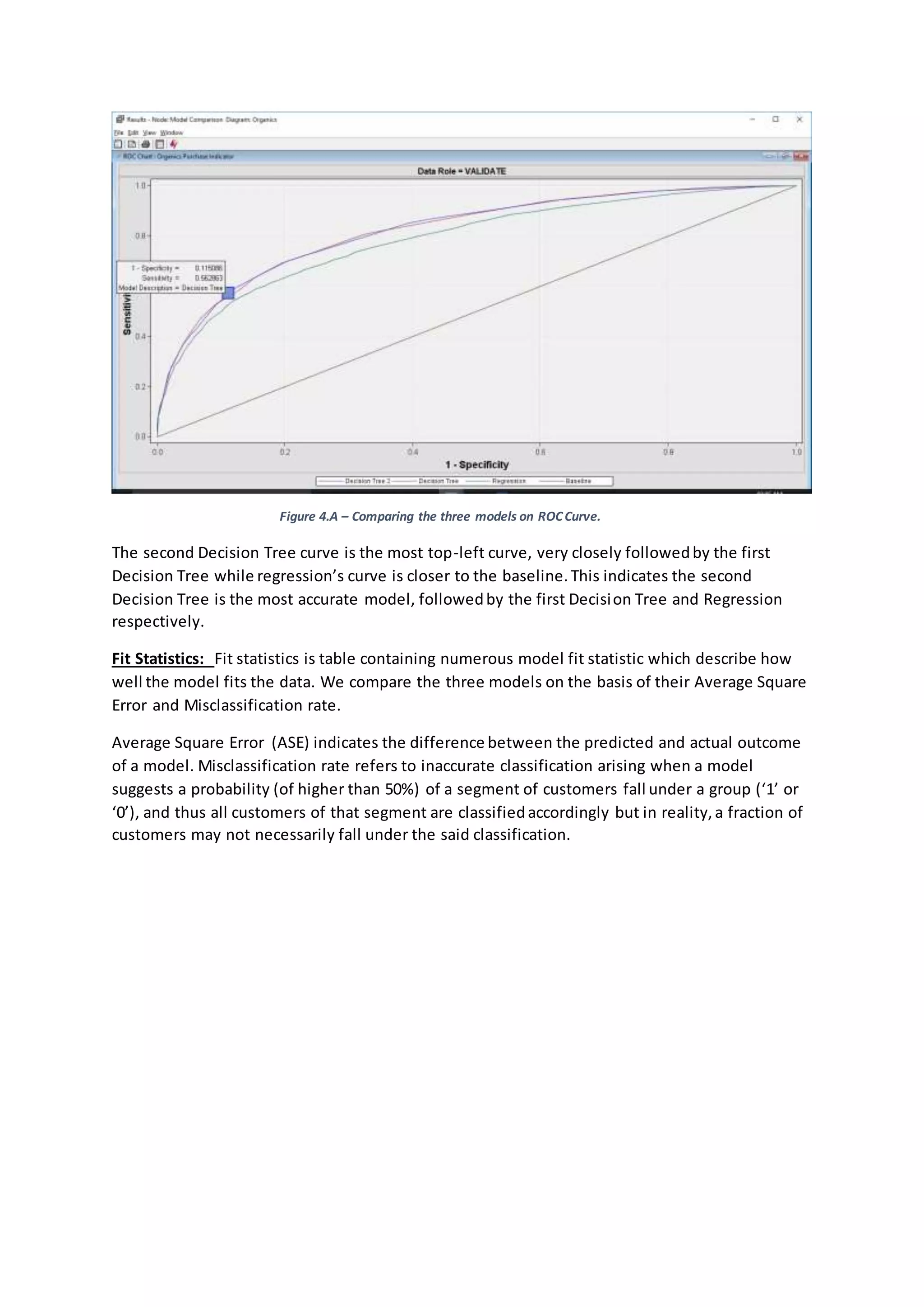
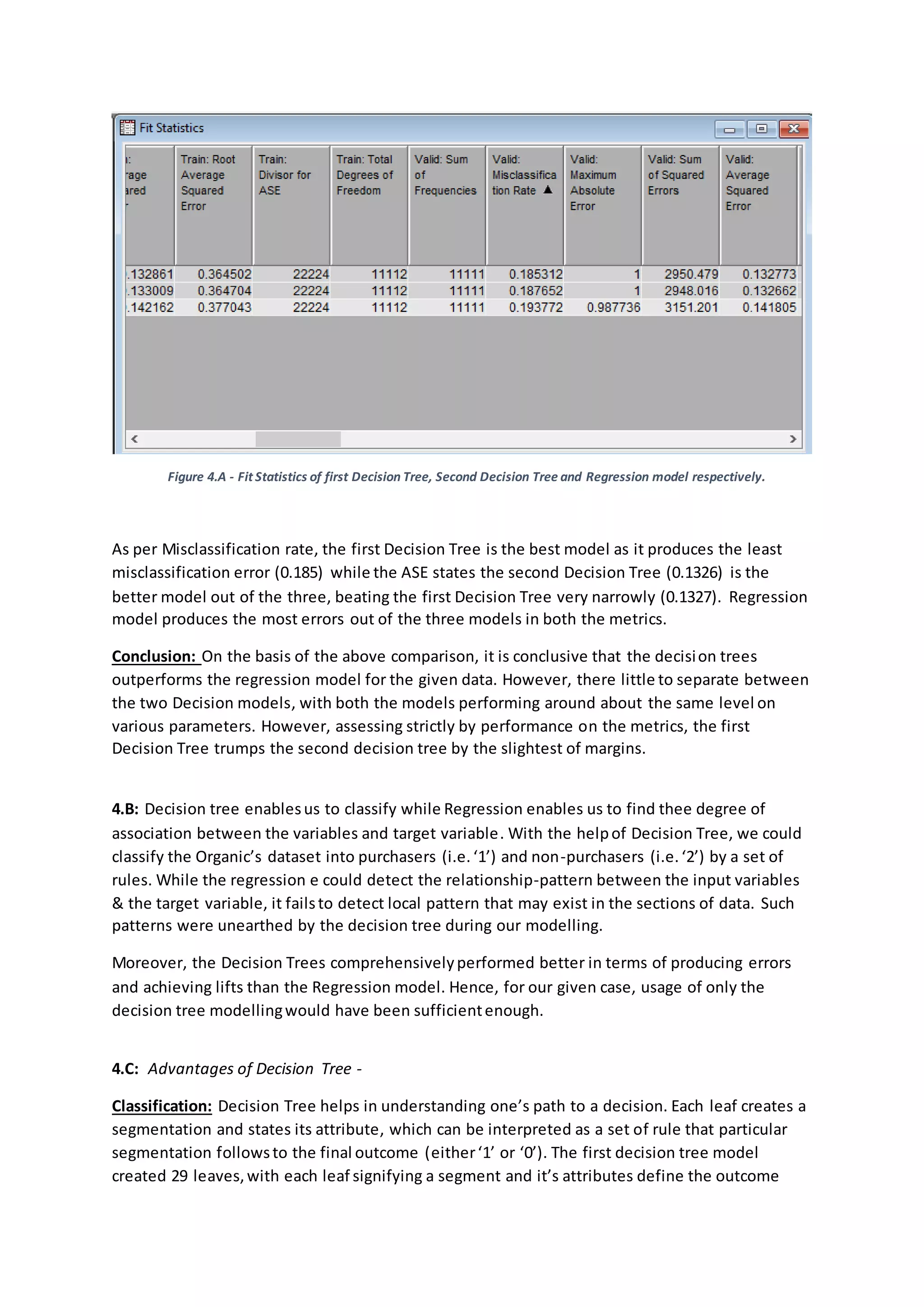
- The document describes building predictive models using decision tree and regression modeling to predict which customers are likely to purchase new organic products being introduced by a supermarket. - Both decision tree and logistic regression models were created, with the decision tree models performing slightly better based on various evaluation metrics such as cumulative lift, ROC curve, and average square error. 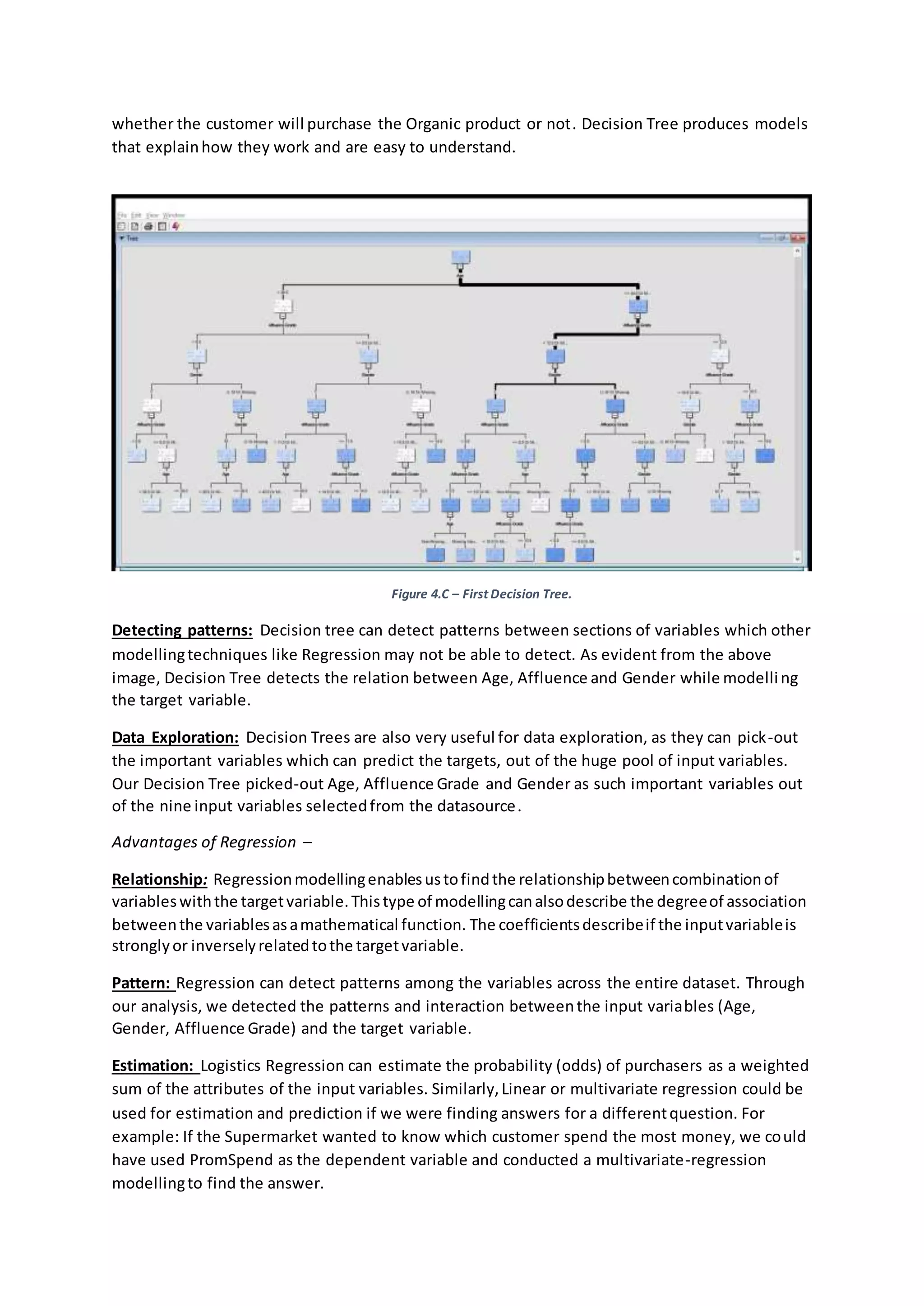- The top variables influencing the likelihood of a customer purchasing organics according to the models were gender, age, and affluence level.

1. Building andEvaluating
Predictivemodel: Supermarket
Business Case
BUS5PA – Assignment 1
SIDDHANTH CHAURASIYA Master of Business Analytics 19139507

2. Objective:
To predict and determine,using Decision Tree and Regression modelling, which segment of
customers are likelyto purchase a new line of organic products that is to be introduced by the
supermarket.
1. Setting up the project and exploratory analysis.
1.A.1&2: On SAS Enterprise Miner workstation, a new Project named
BUS5PA_Assignment1_19139507 is created, followedby creating a diagram called Organics.
Further, a SAS library is created and the given dataset ‘Organics’ is selected as the data source
for the project. On analysing the dataset, SAS Enterprise Miner found 22223 observations and
13 variables.
The roles of the 13 variables have been set as follows:
Figure 1.A.2 - Roles & Measurement Level of Variables
Variables with Nominal Measurement Level contain Categorical data while variables with
Interval Measurement Level contain numeric data. Target/Respond variable TargetBuy has a
Binary Measurement, with 1 indicating Yes and 0 indicating No.

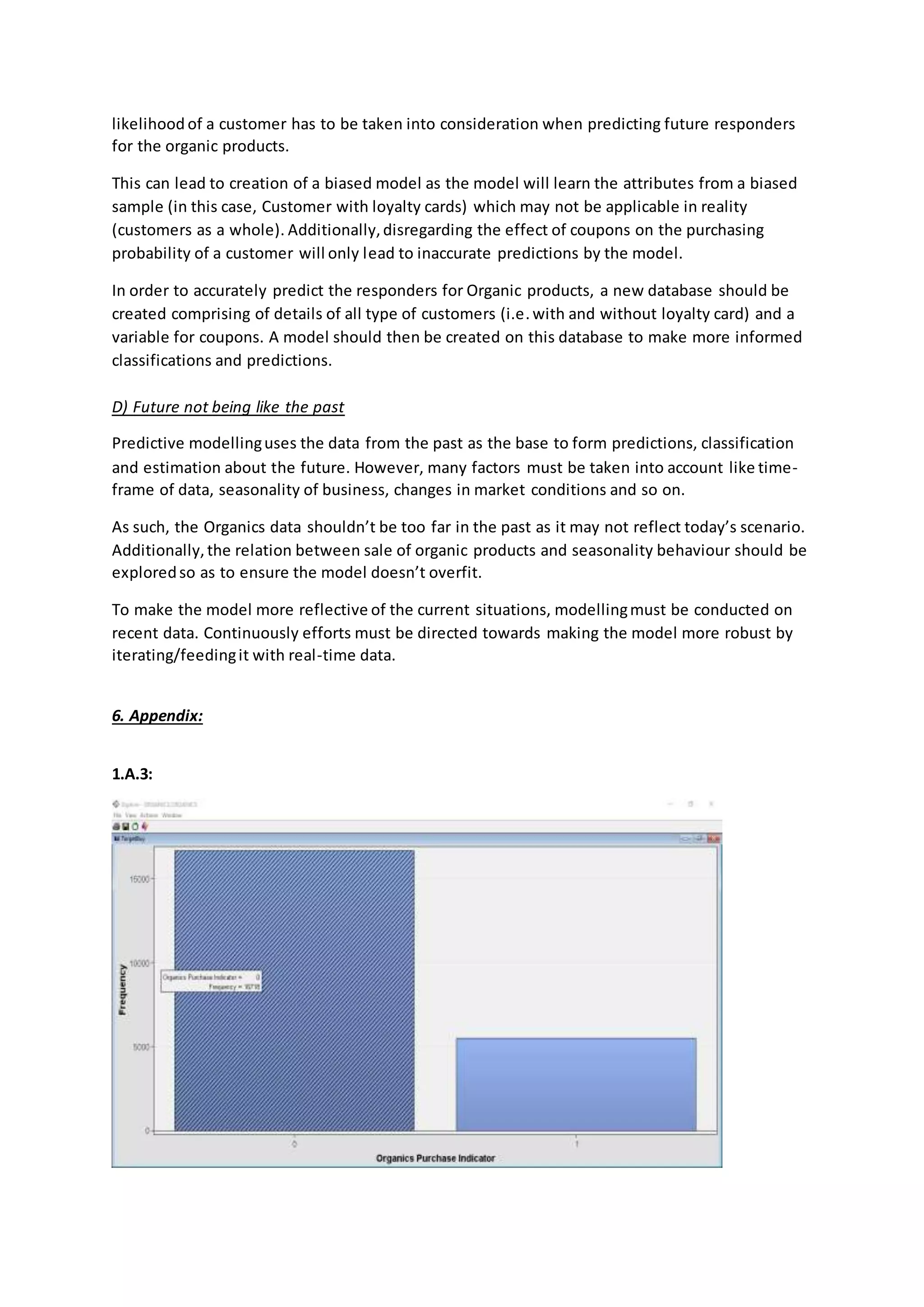
3. 1.A.3: Distribution of Target variables [Appendix – Figure 1.A.3 (2)]
Figure 1.A.3 - Summary of Distribution of TargetBuy
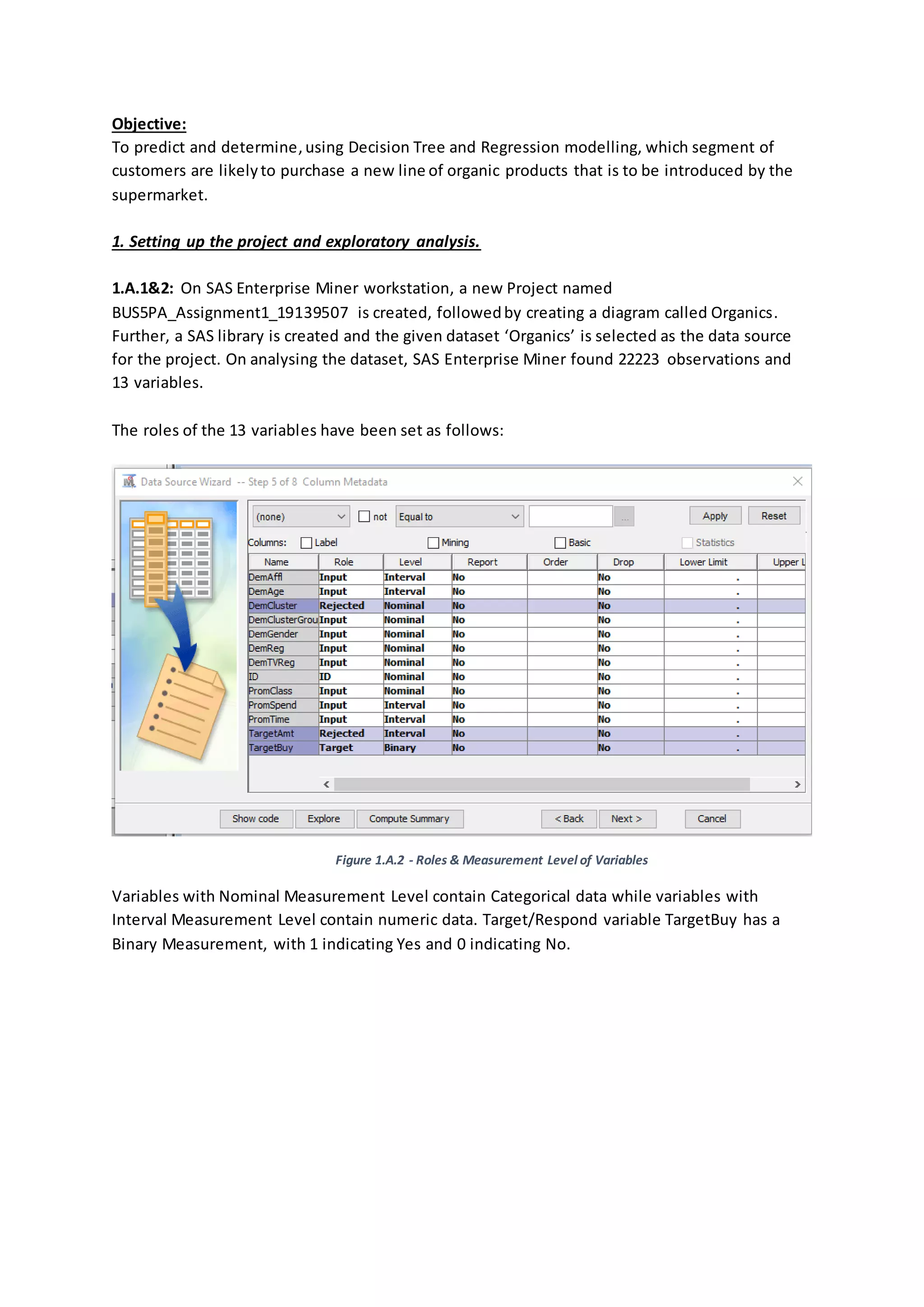
1.A.4: DemCluster has been Rejected as DemClusterGroup contains collapsed data of
DemCluster and based on past evidences,DemClusterGroup is sufficientfor the modelling.
1.B: TargetBuy envelopesthe data contained in TargetAmt. Utilizing TargetAmt as an input
could lead to an imprecise modelling or leakage as the model would find strong co-relation
between the input (TargetAmt) and Target (TargetBuy), since the target variable contains the
collapsed data of TargetAmt. Hence, TargetAmt should not be used as input and should be set
as Rejected.
2. Decision tree based modelling and analysis.
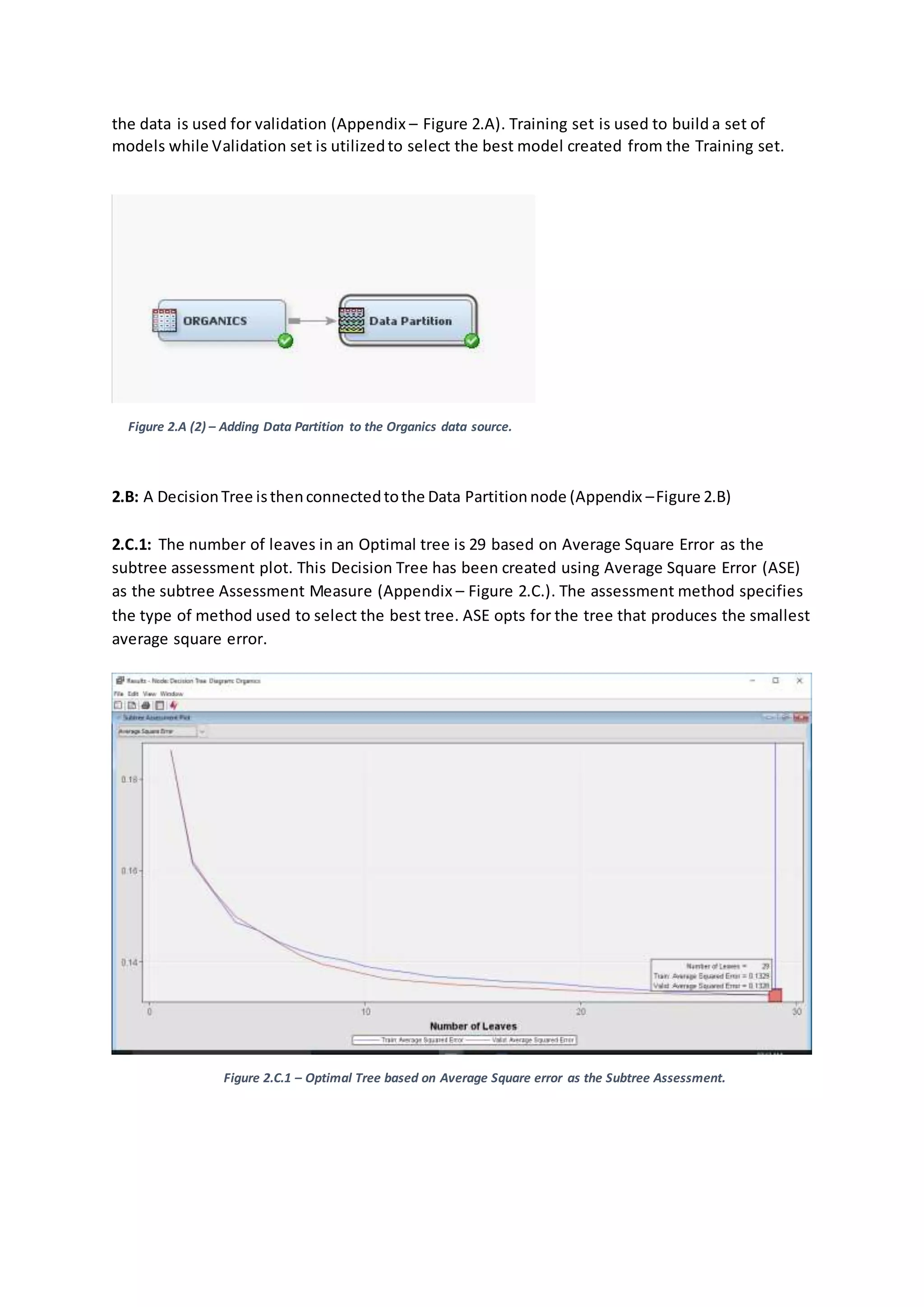
2.A: After dragging the Organics dataset to the Organics diagram, we connect the Data Partition
node to the Organics dataset. 50% of the data is utilizedfor training while the remaining 50% of

4. the data is used for validation (Appendix – Figure 2.A). Training set is used to build a set of
models while Validation set is utilizedto select the best model created from the Training set.
Figure 2.A (2) – Adding Data Partition to the Organics data source.
2.B: A DecisionTree isthenconnectedtothe Data Partition node (Appendix –Figure 2.B)
2.C.1: The number of leaves in an Optimal tree is 29 based on Average Square Error as the
subtree assessment plot. This Decision Tree has been created using Average Square Error (ASE)
as the subtree Assessment Measure (Appendix – Figure 2.C.). The assessment method specifies
the type of method used to select the best tree. ASE opts for the tree that produces the smallest
average square error.
Figure 2.C.1 – Optimal Tree based on Average Square error as the Subtree Assessment.

5. 2.C.2: Variable DemAge was used for the first split as this is the variable which ensures the best
split in terms of ‘Purity’ (Appendix – Figure 2.C.2).
Based on Logworth of each input variable, the competing splits for the first split (DemAge) for
the first decision tree are DemAffl and DemGender. Logworth is measure of Entropy, which
indicates which variable can create the most homogenous subgroups.
Figure 2.C.2 – Logworth of Input Variables
2.D.1: The maximum branches of the second decision tree has been changed to 3. This means
the subsets of the splitting rules are dividedinto 3 branches (Appendix – Figure 2.D.1).
2.D.2: The second Decision Tree has been created using Average Square Error (ASE) as the
subtree Assessment Measure (Appendix – Figure 2.D.2). The assessment method specifiesthe
type of method used to select the best tree. ASE opts for the tree that produces the smallest
average square error.
Figure 2.D.2 (2) – Adding the second Decision Tree node.
2.D.3: The optimal tree for Decision Tree 2 using Average Square Error as the model assessment
statistic contains 33 leaves.

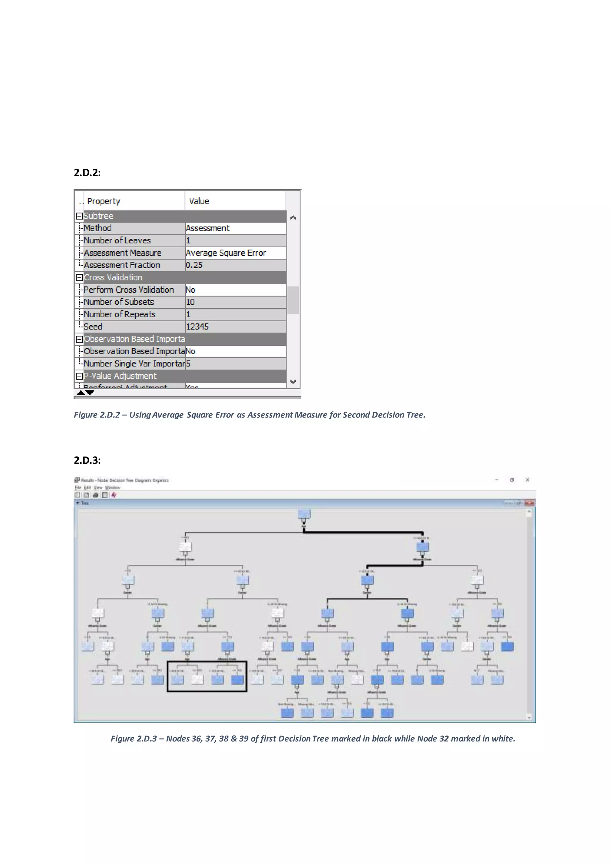
6. Figure 2.D.3 – Leaves on Optimal Tree based on Average Square Error for Decision Tree 2.
The two Decision Tree models differas the maximum branch splits (2 vs 3) is different.This
results in the divergence in number of leavesin optimal tree of the respective Decision Tree the
first decision tree contains 29 leaves whereas Decision Tree 2 contains 33 leaves.
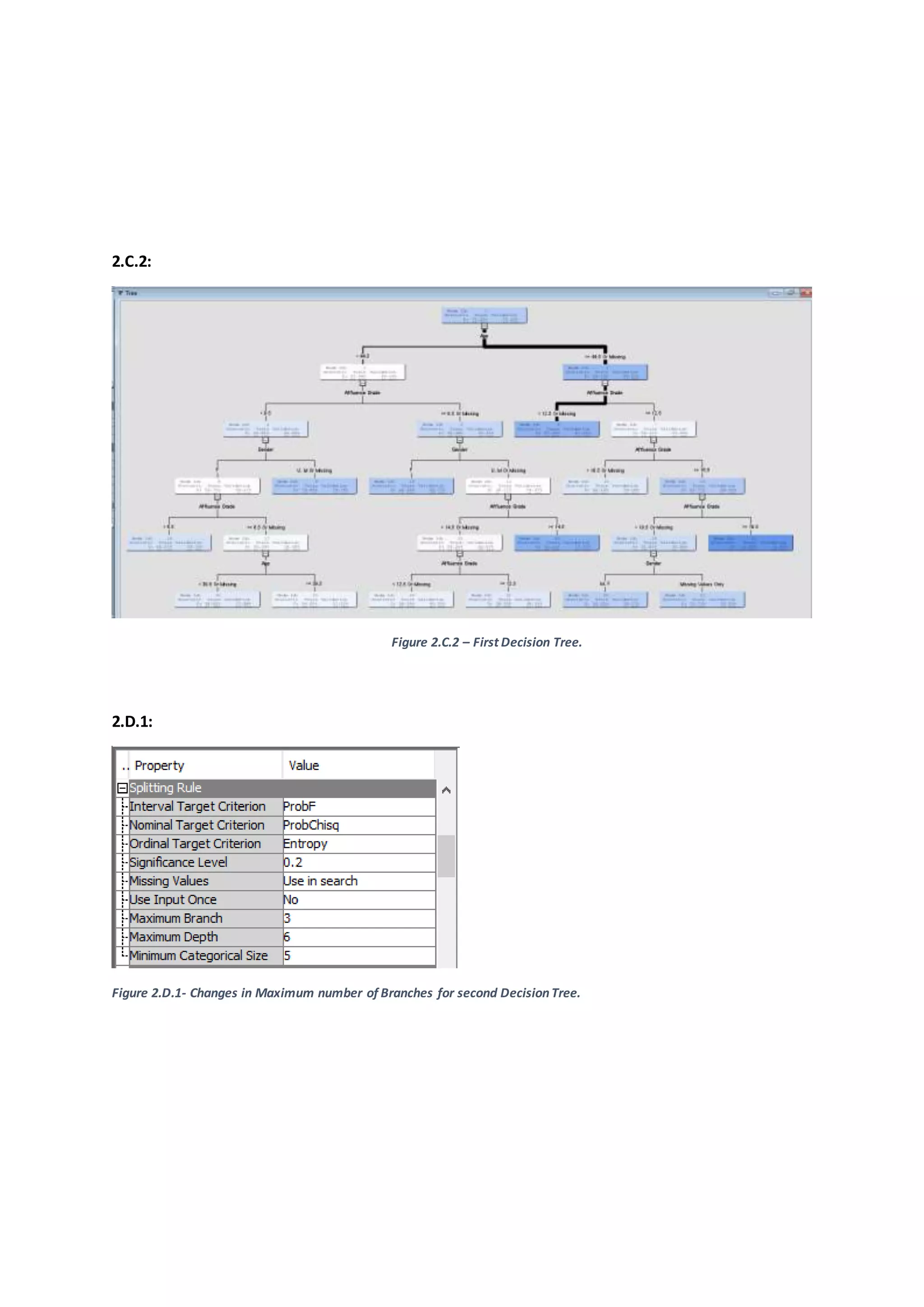
The set of rulesor classificationsetbythe firstDecisionTree canbe summarizedas –
 Female customersunderthe Age of 44.5 years,havingAffluence grade more than9.5 or
missingare likelytopurchase organicproducts(Node 36,37, 38 & 39, Appendix –Figure
2.D.3).
 Female customersunderthe age of 39.5 years,havingAffluence grade of lessthan9.5 but
more than 6.5 or missingare likelytopurchase organicproducts(Node 32, Appendix–
Figure 2.D.3).
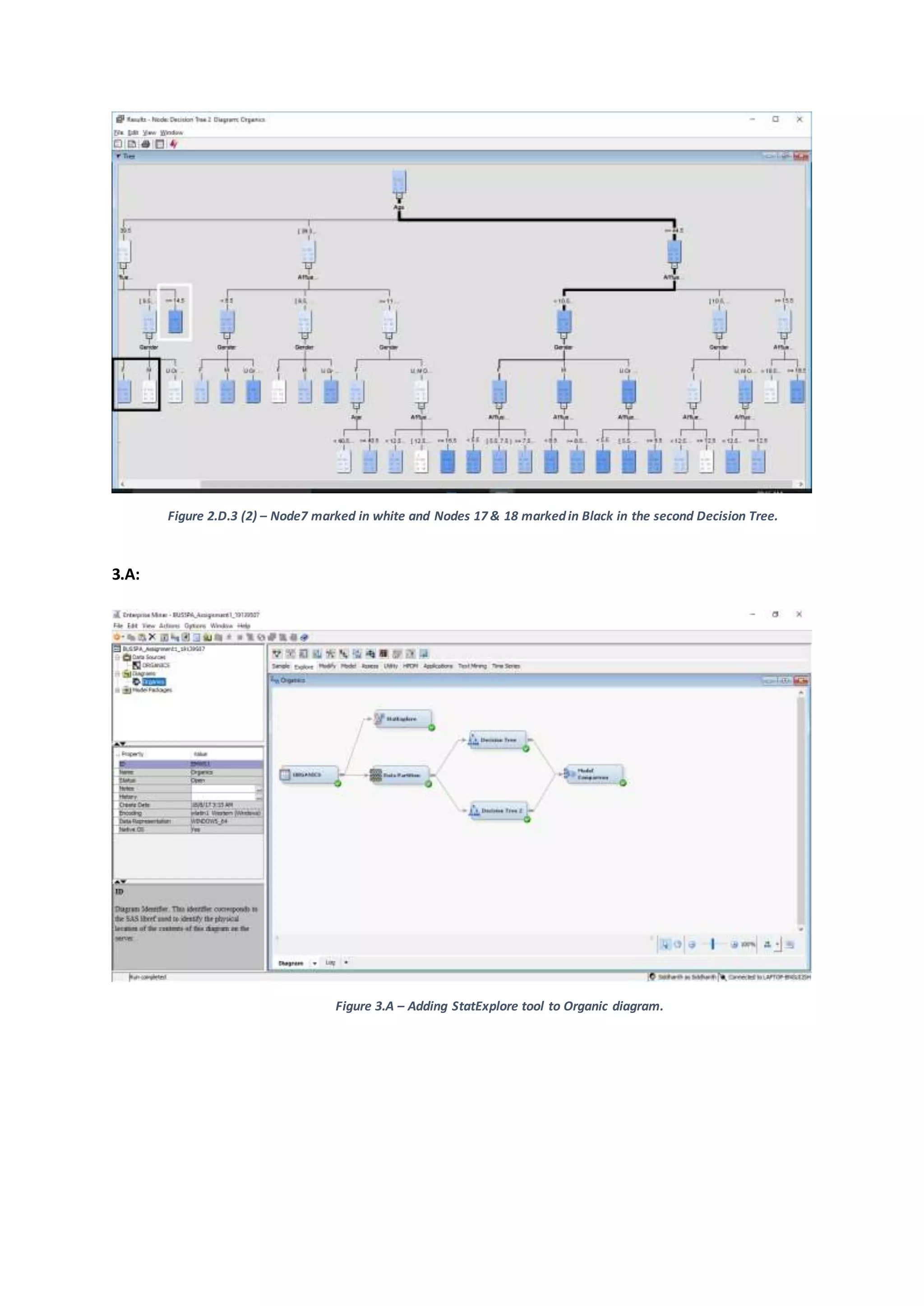
The set of rules or classificationsetbythe secondDecisionTree canbe summarizedas –
 Customersunderthe age of 39.5 yearswhohave an affluence grade of more than14.5 are
verylikelytopurchase organicproducts[Node 7,Appendix –Figure 2.D.3(2)].
 Customersunderthe age of 39.5 yearshavingaffluencegrade of lessthan14.5 butmore
than 9.5 (ormissing) are likelytopurchase organicproducts.However,if suchacustomeris
a Female,thenshe is22% more likelytobuyOrganicproductsthan the customerwhois
male withthe same attributes[Node 17& 18, Appendix –Figure 2.D.3 (2)].
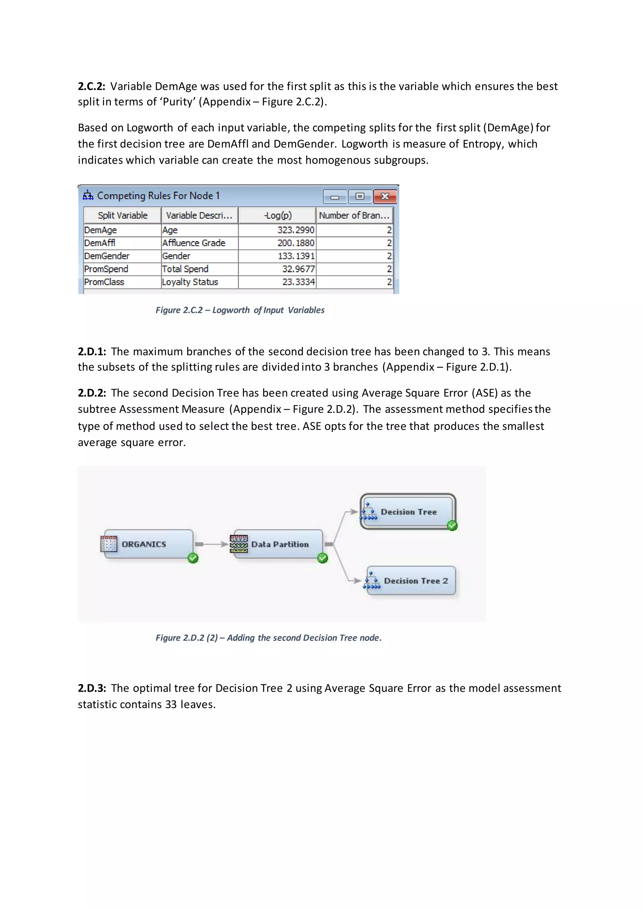
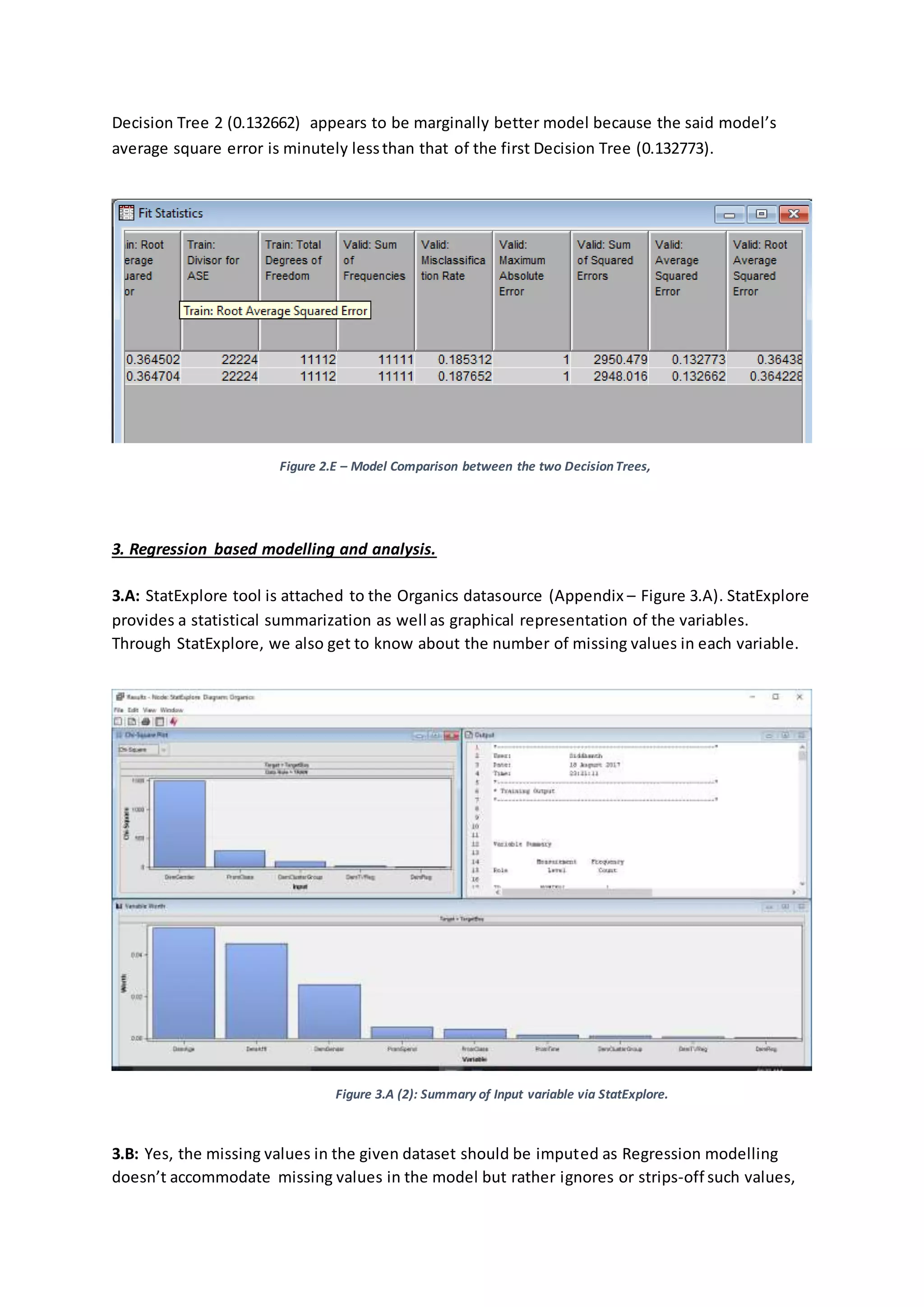
2.E: Average square error computes, squares and then averages the variation betweenthe
predicted outcome and the actual outcome of the leaf nodes. Lower the average square error,
better the model; as it indicates the model produces the fewer errors. For the Organics dataset,

7. Decision Tree 2 (0.132662) appears to be marginally better model because the said model’s
average square error is minutely lessthan that of the first Decision Tree (0.132773).
Figure 2.E – Model Comparison between the two DecisionTrees,
3. Regression based modelling and analysis.
3.A: StatExplore tool is attached to the Organics datasource (Appendix – Figure 3.A). StatExplore
provides a statistical summarization as well as graphical representation of the variables.
Through StatExplore, we also get to know about the number of missing values in each variable.
Figure 3.A (2): Summary of Input variable via StatExplore.
3.B: Yes, the missing values in the given dataset should be imputed as Regression modelling
doesn’t accommodate missing values in the model but rather ignores or strips-off such values,

8. thereby leading to loss of data to that extent for the modelling. This can lead to a creation of
biased training set.
Imputation for Decision Tree isn’t required as Decision Tree accommodates the missing values in
its modellingby considering them as a possible value with its own branch.
3.C: We add impute node to the diagram and connect it to the Data Partition node (Appendix –
Figure 3.C). Impute function creates a synthetic value for the missing value. We impute alphabet
‘U’ for missing class variable value and use the mean of the variable to impute missing interval
variable values.
Figure 3.C – Results of Impute.
We then create imputation indicators for all imputed inputs. This function creates a new
variable to indicate whether a value has been imputed or not in the main variable.
3.D: We adda Variable Clustering node toImpute node togrouptogethersimilarvariablesina
cluster(Appendix –Figure 3.D).Byvirtue of Impute’sfunction, new inputvariablesare created
containingthe imputedvalues forthe missingvalues.Similarly,new indicatorvariableshave also
beencreated. VariableClusteringenablesustoreduce redundancyandensure betterregression
basedmodellingasthistype of modellingismore suitedwheninputvariablesare fewer.
Each clusteris representedbyanindividual inputvariable.We optforBest Variable asthe criteria
for the selectionforthe clusterrepresentative.The variablewith the lowestnormalisedvalue of R
squaredisselectedasthe clusterrepresentative underthe Bestvariable method.
As a result,the 52 variables(afterimputationandindicatorvariables)are groupedtogethertoform
24 clusters.The clusterrepresentativesof the 24 clusterswill be thenusedasthe inputsforthe

9. Regressionmodel.
Figure 3.D (2) – Representation of Variable Clustering in various forms.
We add Regression node to the Variable clustering node and change the Selectionmodel to
Stepwise and Selection criterion to Validation Error. Under the Stepwise model, variables are
added one by one to the model.At the same time as the addition, the variable already in the
model whose Stay Significance level falls below the threshold is deleted.This type of model
stops when the Stay Significance level or Selectioncriterion (Validation Error in this case) is
achieved.
Figure 3.E – Adding Regression node and changing its properties.

10. The measurement of Target variable determinesthe type of Regression model that will be
applied. For our given case, Logistic Regression model will be used as our Target Variable is
Binary.
3.F.1: The variables included in the final model of the Regression modellingare:
 IMP_DemAffl – Imputed Affluence Grade.
 IMP_DemAge – Imputed Age.
 M_DemGender0 – Indicator Gender.
 IMP_DemGenderM – Imputed Gender.
 M_DemAffl0 – Indicator Affluence Grade.
 M_DemAge0 – Indicator Age.
The regression modellingindicates the above-mentioned variables have a significant degree
of association with our target variable. The list of variables is in order of their stepwise
addition to the model.
Regression models enables us to estimate the relationshipbetween the input variables and
target variable. Logistics regression helpsus to expressthe association betweenthe input
and target variable in terms of odds (Purchaser vs Non-purchaser)
The higher management of supermarket can interpret the abovementioned association as
follows:
Figure 3.F.1 – Variables in final Logistic Regression model.
With other variables constant, change in a single unit in IMP_DemAffl will result in a 0.2530-unit
change in the log odds of purchaser (vs non-purchaser). On the other hand, with other variables
constant, a change of a single unit in IMP_DemAge will lead to a decrease in log odds by 0.0550.
Similarly, with other variables constant increase in a single unit of IMP_DemGenderM,
M_DemAffl0 and M_DemAge0 will result in decrease in the log odds of a purchaser by 0.7277,
0.3657 and 0.2345 unit respectivelywhile increase in a single unit of M_DemGender0 will lead
to increase in log odds of purchasers by 1.41 units.

11. 3.F.2: The most important variables that influence the target variable are M_DemGender0,
IMP_DemGenderM and M_DemAffl0 respectively.These variables are designated their
importance on the basis of their Absolute Coefficients.
Absolute coefficientsspecifieshow strongly related the variable is related to the target variable.
Variables with Absolute coefficientcloser to 1 indicate strong positive relationship,while
absolute coefficient of around abound -1 indicates strong negative relation. An absolute
coefficientof zero impliesthe weakest relation betweenthe input variable and target variable
for the given scenario.
Figure 3.F.2 – Bar-chart and tabular form of most important variables for Regression modelling.
The bar chart when interpreted together suggests that female customers who are of relatively
young age and have an high affluence grade tend to purchase more Organic products.
3.F.3: The validation Average Square Error (ASE) for the Regression model is 0.141805. ASE helps
in gauging which model is erroneous less often than the other. Lesser ASE indicates better
model in terms of its prediction capabilities. ASE is calculated by squaring and averaging the
difference between the predicted and actual outcome for each and every model.
The ASE is the lowest at the model selectionstep number 6, which impliesthis is the most
optimal model, as shown in the below chart.

12. Figure 3.F.3 – Validation Average Square Error of Logistic Regression model.
4. Open ended discussion (20%)
4.A: A model comparison tool is added to the workspace and the decision trees & regression
nodes are attached to model comparison. This node enables us to compare the models and its
predictive capabilities.
Figure 4.A – Adding Comparison node to the workspace.

13. We use three metrics to ascertain which model outperformed the other models on the
validation dataset. These metrics are: Cumulative Lift, ROC Curve and Fit statistics (Average
Square Error and Misclassification rate).
Cumulative Lift: Lift curve measures the effectivenessof the model by comparing the results
obtained with and without the predicted model. The first Decision tree (3.42) performs
marginally better than the second Decision Tree (3.40) on the metric of cumulative gain at the
5th
percentile,while the regression model gives a liftof 3.34 at the 5th
depth.
Figure 4.A – Comparing the three models on Cumulative Lift Chart.
This is interpreted as the top 5% of customers picked by the first Decision Tree model are 3.42
times more likelyto purchase Organic products than the 5% of customers picked out at random.
ROC Curve: ROC curve is graph that demonstrates the relation between Sensitivity(True
positive) and Specificity(True negative) at varied points of a diagnostic test. The model’s curve
which is closer to the top and the left (i.e.closer to the true positive) can predict more
accurately, while the curve which is inclinedtowards the baseline (i.e.closer to the true
negative) is a lesser accurate predictor. From a business context, the supermarket would
naturally want to adopt the curve that inclinestowards the Sensitivity.

14. Figure 4.A – Comparing the three models on ROCCurve.
The second Decision Tree curve is the most top-left curve, very closely followedby the first
Decision Tree while regression’s curve is closer to the baseline.This indicates the second
Decision Tree is the most accurate model, followedby the first Decision Tree and Regression
respectively.
Fit Statistics: Fit statistics is table containing numerous model fit statistic which describe how
well the model fits the data. We compare the three models on the basis of their Average Square
Error and Misclassification rate.
Average Square Error (ASE) indicates the difference between the predicted and actual outcome
of a model. Misclassification rate refers to inaccurate classification arising when a model
suggests a probability (of higher than 50%) of a segment of customers fall under a group (‘1’ or
‘0’), and thus all customers of that segment are classifiedaccordingly but in reality,a fraction of
customers may not necessarily fall under the said classification.

15. Figure 4.A - Fit Statistics of first Decision Tree, Second Decision Tree and Regression model respectively.
As per Misclassification rate, the first Decision Tree is the best model as it produces the least
misclassification error (0.185) while the ASE states the second Decision Tree (0.1326) is the
better model out of the three, beating the first Decision Tree very narrowly (0.1327). Regression
model produces the most errors out of the three models in both the metrics.
Conclusion: On the basis of the above comparison, it is conclusive that the decision trees
outperforms the regression model for the given data. However, there little to separate between
the two Decision models, with both the models performing around about the same level on
various parameters. However, assessing strictly by performance on the metrics, the first
Decision Tree trumps the second decision tree by the slightest of margins.
4.B: Decision tree enablesus to classify while Regression enables us to find thee degree of
association between the variables and target variable. With the helpof Decision Tree, we could
classify the Organic’s dataset into purchasers (i.e.‘1’) and non-purchasers (i.e.‘2’) by a set of
rules. While the regression e could detect the relationship-pattern between the input variables
& the target variable, it failsto detect local pattern that may exist in the sections of data. Such
patterns were unearthed by the decision tree during our modelling.
Moreover, the Decision Trees comprehensivelyperformed better in terms of producing errors
and achieving lifts than the Regression model. Hence, for our given case, usage of only the
decision tree modellingwould have been sufficientenough.
4.C: Advantages of Decision Tree -
Classification: Decision Tree helps in understanding one’s path to a decision. Each leaf creates a
segmentation and states its attribute, which can be interpreted as a set of rule that particular
segmentation followsto the final outcome (either‘1’ or ‘0’). The first decision tree model
created 29 leaves,with each leaf signifying a segment and it’s attributes define the outcome

16. whether the customer will purchase the Organic product or not. Decision Tree produces models
that explainhow they work and are easy to understand.
Figure 4.C – First Decision Tree.
Detecting patterns: Decision tree can detect patterns between sections of variables which other
modellingtechniques like Regression may not be able to detect. As evident from the above
image, Decision Tree detects the relation between Age, Affluence and Gender while modelling
the target variable.
Data Exploration: Decision Trees are also very useful for data exploration, as they can pick-out
the important variables which can predict the targets, out of the huge pool of input variables.
Our Decision Tree picked-out Age, Affluence Grade and Gender as such important variables out
of the nine input variables selectedfrom the datasource.
Advantages of Regression –
Relationship: Regressionmodellingenablesustofindthe relationshipbetweencombinationof
variableswiththe targetvariable.Thistype of modellingcanalsodescribe the degreeof association
betweenthe variablesasamathematical function. The coefficientsdescribeif the inputvariableis
stronglyor inverselyrelatedtothe targetvariable.
Pattern: Regression can detect patterns among the variables across the entire dataset. Through
our analysis, we detected the patterns and interaction betweenthe input variables (Age,
Gender, Affluence Grade) and the target variable.
Estimation: Logistics Regression can estimate the probability (odds) of purchasers as a weighted
sum of the attributes of the input variables. Similarly,Linear or multivariate regression could be
used for estimation and prediction if we were finding answers for a differentquestion. For
example: If the Supermarket wanted to know which customer spend the most money, we could
have used PromSpend as the dependent variable and conducted a multivariate-regression
modellingto find the answer.

17. 5. Extending current knowledge with additional reading (15%)
A) Just getting things wrong
Addressing the wrong issue can render the entire data mining process futile as no or little
business value can be derived from the solutions obtained from the modelling.
As such, understanding the businessproblem and addressing the correct issue becomes
imperative. Such a situation could arise at the supermarket if the higher management frame the
wrong question or attempt to try and solve the wrong problem. In our case, this could happen if
an incorrect target variable is selected.Similarly, wrongly rejecting a potentially important
variable could lead to a creation of a skewedmodel. These issues can be resolvedby having a
person in-charge of the project with the right domain expertise to complement with technical
know-hows.
Erroneous interpretation of binary ‘0’ and ‘1’ by team-members could potentiallylead to a
complete failure of the modelling. Such incidents can be solved by having transparent
communication across the hierarchy of the supermarket and standardization of processes and
rules.
B) Overfitting
Overfitting is phenomena which occurs when a model learns the details, noises or fluctuations
in the training set too well.Such a model memorizes those detailsrather than learning, and then
applies them to a new dataset where it isn’t applicable, leading to poor predictive performance.
A model can be assessed whether it is overfitting or not by evaluating the Average Square Error
and Misclassification rate graphs. If the training performance improves and validation
performance deteriorates, in terms of Average Square Error or Misclassification rate, as the
complexity of the model increases, the model shows signs of overfitting.
Overfitting can arise in our model created for the supermarket, if the model recognizes or
memorizes bogus patterns which aren’t applicable to other data sources. Overfittingcan also
appear when the training set allocated for our supermarket analysis is not sufficientlylarge.
Overfitting leads to creation of unstable model that may perform on some days and may not on
other occasions.
Such a model can be avoided by including only those variables which have a predictive value.
Additionally, allocating an optimal proportion of dataset for the model to train can help to
combat the problem of overfitting.
C) Sample bias
Sampling bias occurs when a sample does not accurately reflect the parent population. The
organics dataset contains details of customers with loyalty card who purchased organic products
on being incentivisedwith coupons. Customers with loyalty card may not be an accurate
representation of the total customer base. Further, the effect of coupons on the purchasing

18. likelihood of a customer has to be taken into consideration when predicting future responders
for the organic products.
This can lead to creation of a biased model as the model will learn the attributes from a biased
sample (in this case, Customer with loyalty cards) which may not be applicable in reality
(customers as a whole). Additionally,disregarding the effect of coupons on the purchasing
probability of a customer will only lead to inaccurate predictions by the model.
In order to accurately predict the responders for Organic products, a new database should be
created comprising of details of all type of customers (i.e.with and without loyalty card) and a
variable for coupons. A model should then be created on this database to make more informed
classifications and predictions.
D) Future not being like the past
Predictive modellinguses the data from the past as the base to form predictions, classification
and estimation about the future. However, many factors must be taken into account like time-
frame of data, seasonality of business, changes in market conditions and so on.
As such, the Organics data shouldn’t be too far in the past as it may not reflect today’s scenario.
Additionally,the relation between sale of organic products and seasonality behaviour should be
exploredso as to ensure the model doesn’t overfit.
To make the model more reflective of the current situations, modellingmust be conducted on
recent data. Continuously efforts must be directed towards making the model more robust by
iterating/feedingit with real-time data.
6. Appendix:
1.A.3:

19. Figure 1.A.3 (2) - Bar-Chart Distribution of TargetBuy
2.A:
Figure 2.A - Data Partition: 50% for Training & 50% for Validation
2.B:
Figure 2.B – Adding DecisionTree node.
2.C.1:
Figure 2.C.1 – Using Average Square Error as Assessment Measure for First DecisionTree.

20. 2.C.2:
Figure 2.C.2 – First Decision Tree.
2.D.1:
Figure 2.D.1- Changes in Maximum number of Branches for second DecisionTree.

21. 2.D.2:
Figure 2.D.2 – UsingAverage Square Error as Assessment Measure for Second Decision Tree.
2.D.3:
Figure 2.D.3 – Nodes 36, 37, 38 & 39 of first DecisionTree marked in black while Node 32 marked in white.

22. Figure 2.D.3 (2) – Node7 marked in white and Nodes 17 & 18 markedin Black in the second Decision Tree.
3.A:
Figure 3.A – Adding StatExplore tool to Organic diagram.

23. 3.C:
Figure 3.C – Adding Impute node and changing functions in the property panel.
3.D:
Figure 3.D – Adding Variable Clustering node and changing its property.