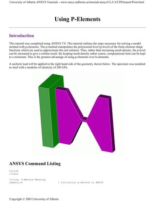
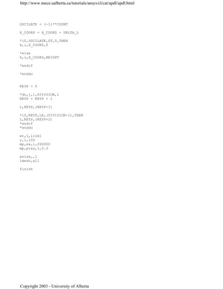
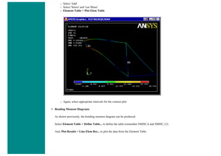
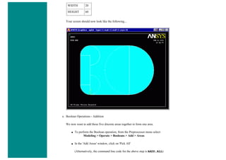
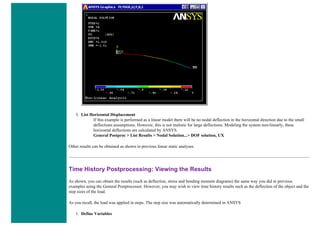
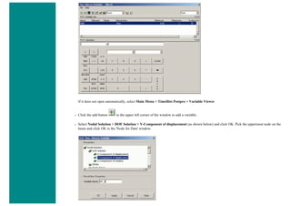
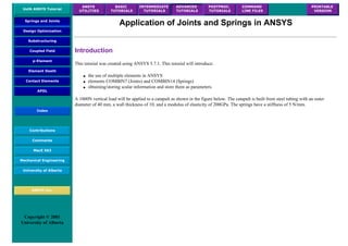
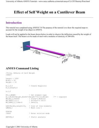
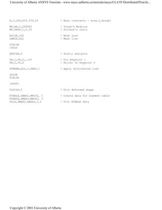
The University of Alberta's ANSYS tutorial offers a comprehensive guide on using ANSYS, a finite element modeling software for mechanical problems such as structural analysis and heat transfer. It is structured into sections that include utilities, basic to advanced tutorials, and command line files, providing step-by-step instructions and explanations tailored for different user proficiency levels. Users are encouraged to practice sequentially through the tutorials to build on skills progressively while being mindful of potential changes across software versions.


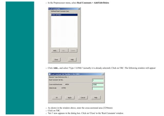
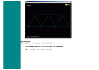
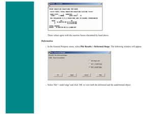
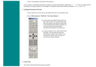
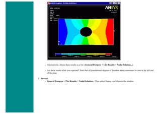
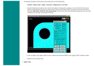
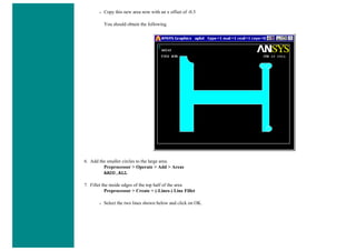
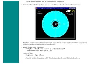
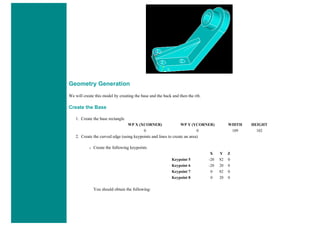
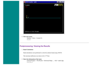
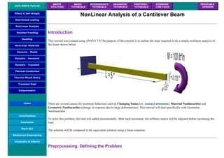
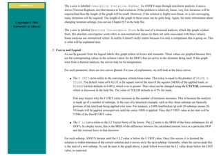
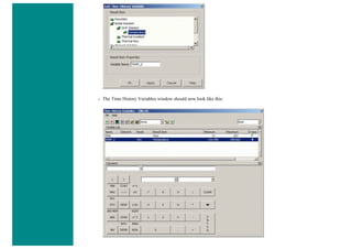
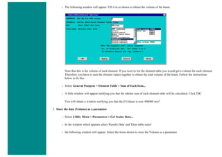
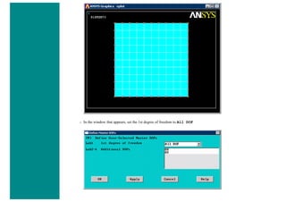
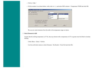
![❍ Click on 'OK'.
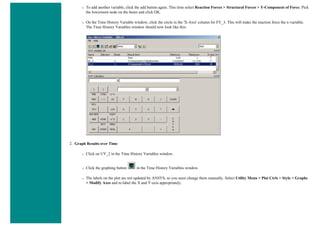
❍ 'Set 1' now appears in the dialog box. Click on 'Close' in the 'Real Constants' window.
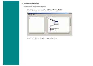
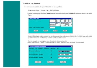
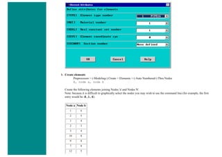
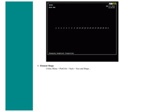
6. Element Material Properties
You then need to specify material properties:
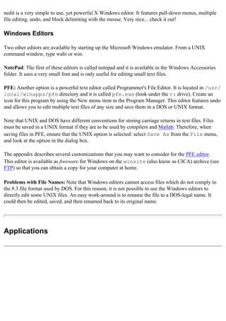
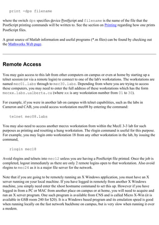
❍ In the 'Preprocessor' menu select Material Props > Material Models...
❍ Double click Structural > Linear > Elastic and select 'Isotropic' (double click on it)
❍ Close the 'Define Material Model Behavior' Window.
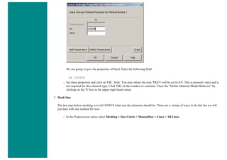
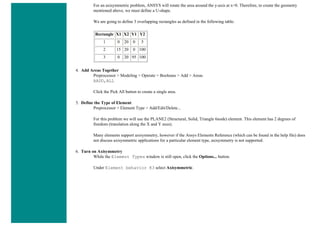
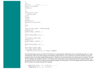
We are going to give the properties of Aluminum. Enter the following field:
EX 70000
PRXY 0.33
❍ Set these properties and click on 'OK'.
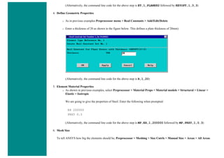
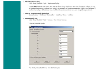
7. Mesh Size
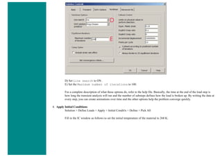
❍ In the Preprocessor menu select Meshing > Size Cntrls > ManualSize > Lines > All Lines
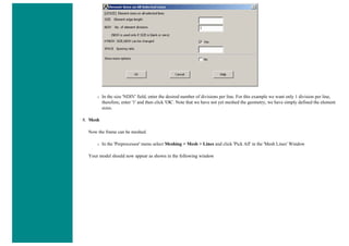
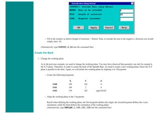
❍ In the size 'SIZE' field, enter the desired element length. For this example we want an element length of 2cm, therefore, enter
'20' (i.e 20mm) and then click 'OK'. Note that we have not yet meshed the geometry, we have simply defined the element sizes.
(Alternatively, we could enter the number of divisions we want in the line. For an element length of 2cm, we would enter 25 [ie
25 divisions]).
NOTE
It is not necessary to mesh beam elements to obtain the correct solution. However, meshing is done in this case so that we can obtain
results (ie stress, displacement) at intermediate positions on the beam.
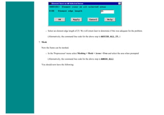
8. Mesh
Now the frame can be meshed.
❍ In the 'Preprocessor' menu select Meshing > Mesh > Lines and click 'Pick All' in the 'Mesh Lines' Window
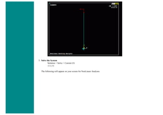
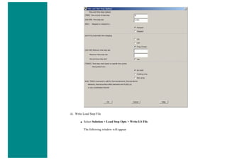
9. Saving Your Work](https://image.slidesharecdn.com/univansystutorialsrameesram-240325071613-ff608449/85/Universal-Ansys-Tutorials-Ramees-Ram-pdf-79-320.jpg)


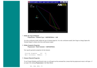
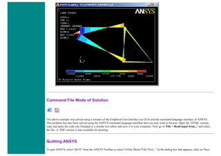


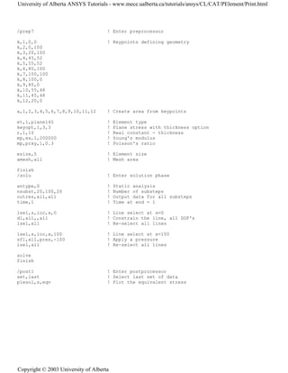
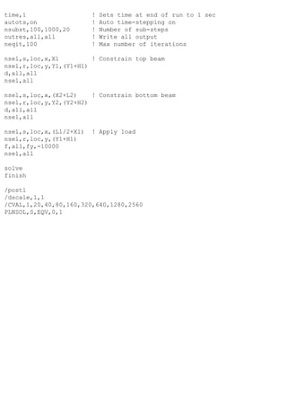
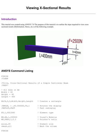
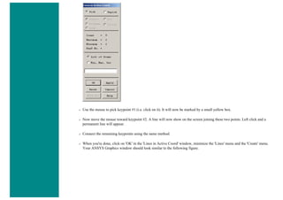
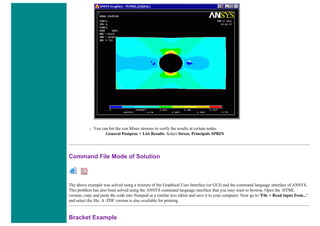
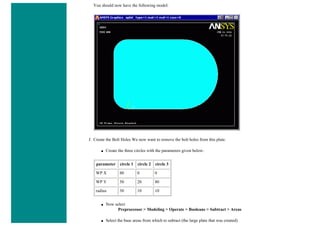
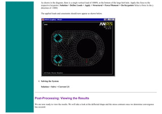
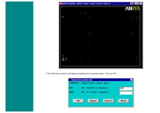
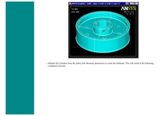
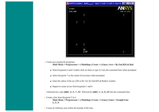
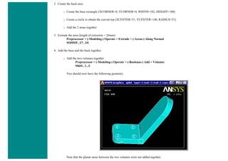
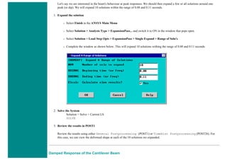
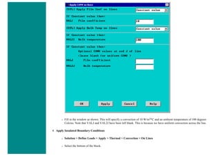
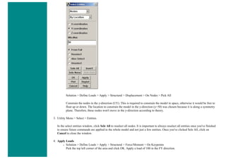
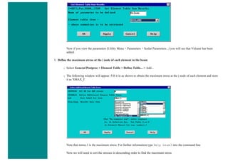
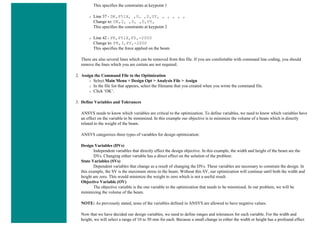
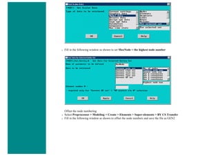
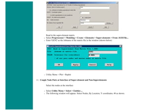
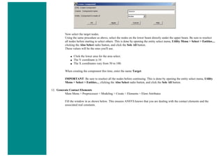
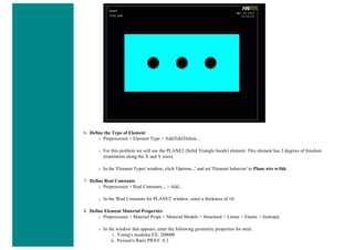
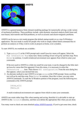
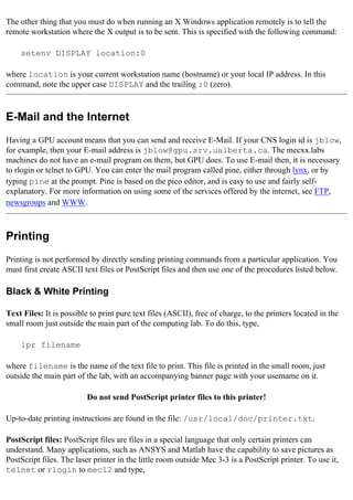
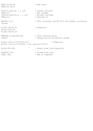
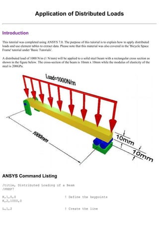
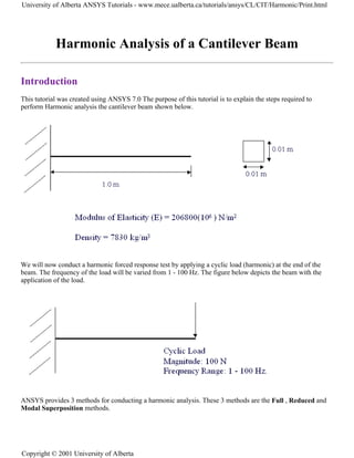
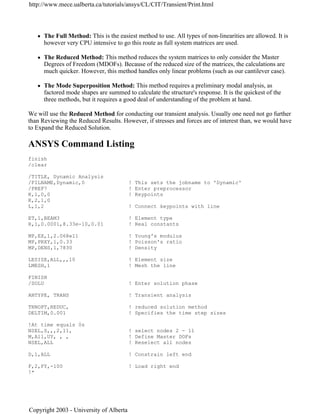
![■ To perform the Boolean operation, from the Preprocessor menu select:
Modeling > Operate > Booleans > Subtract > Areas
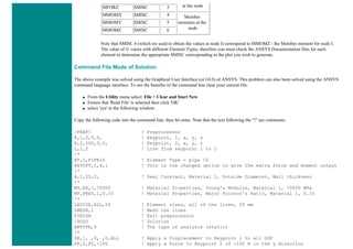
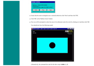
■ At this point a 'Subtract Areas' window will pop up and the ANSYS Input window will display the following
message: [ASBA] Pick or enter base areas from which to subtract (as shown below)
■ Therefore, select the base area (the rectangle) by clicking on it. Note: The selected area will turn pink once it is
selected.
■ The following window may appear because there are 2 areas at the location you clicked.](https://image.slidesharecdn.com/univansystutorialsrameesram-240325071613-ff608449/85/Universal-Ansys-Tutorials-Ramees-Ram-pdf-112-320.jpg)
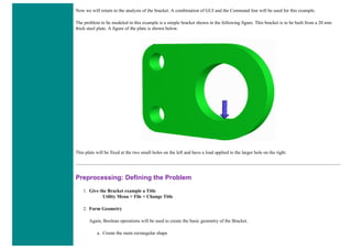
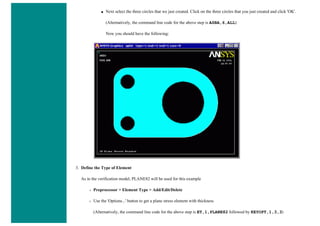


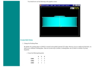
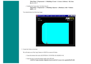


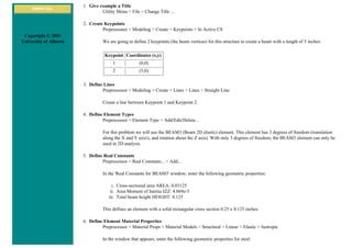


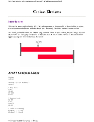
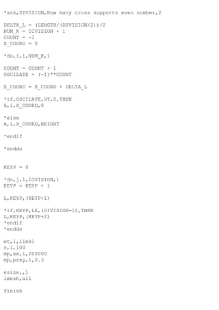
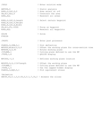
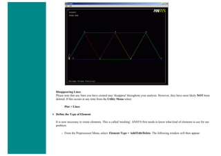
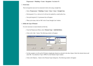
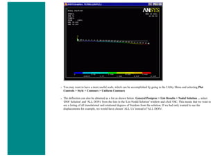
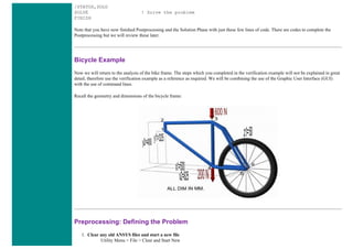
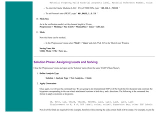
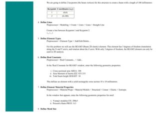
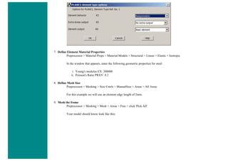
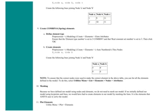
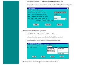
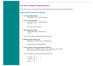
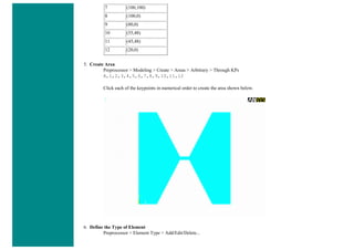
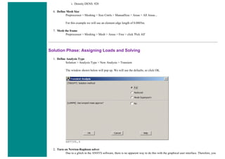
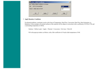
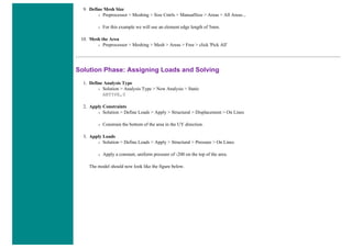
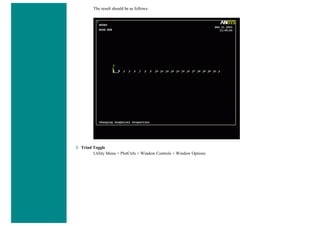
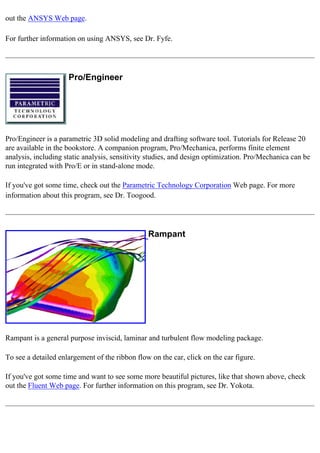
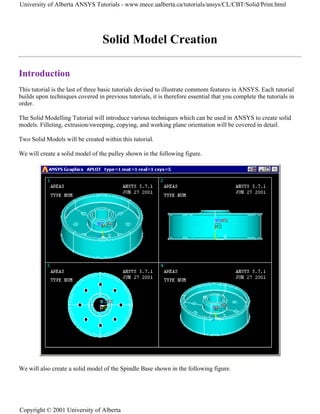
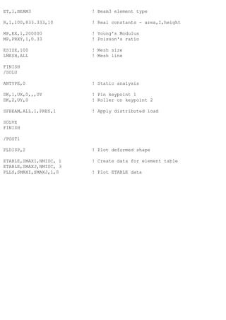
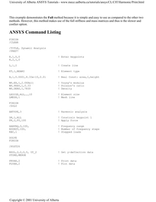
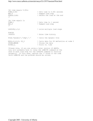
![8. Define Mesh Size
Preprocessor > Meshing > Size Cntrls > ManualSize > Lines > All Lines...
For this example we will specify an element edge length of 10 mm (10 element divisions along the line).
9. Mesh the frame
Preprocessor > Meshing > Mesh > Lines > click 'Pick All'
LMESH,ALL
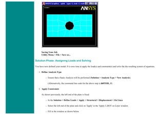
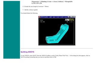
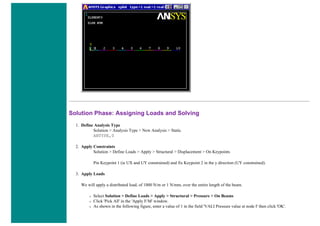
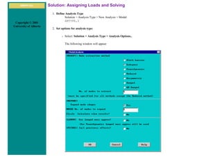
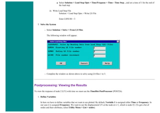
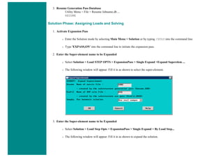
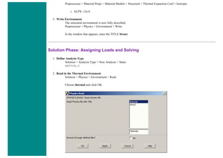
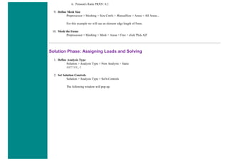
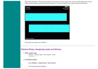
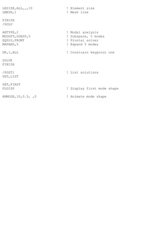
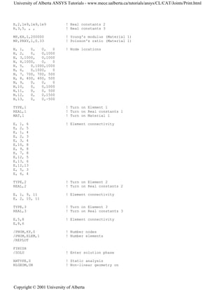
Solution Phase: Assigning Loads and Solving
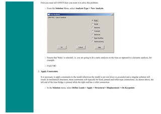
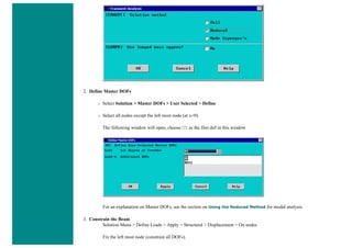
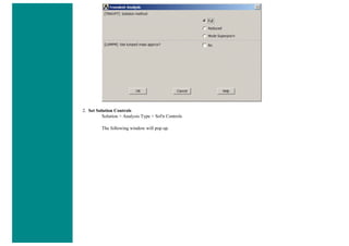
1. Define Analysis Type
Solution > Analysis Type > New Analysis > Static
ANTYPE,0
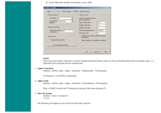
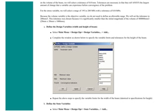
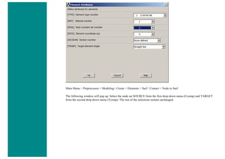
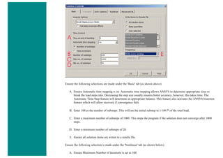
2. Activate prestress effects
To perform an eigenvalue buckling analysis, prestress effects must be activated.
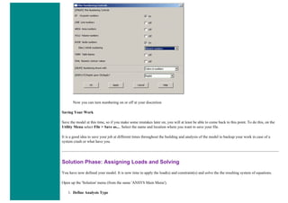
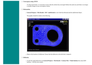
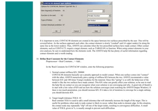
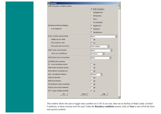
❍ You must first ensure that you are looking at the unabridged solution menu so that you can select Analysis Options in the
Analysis Type submenu. The last option in the solution menu will either be 'Unabridged menu' (which means you are
currently looking at the abridged version) or 'Abriged Menu' (which means you are looking at the unabridged menu). If you
are looking at the abridged menu, select the unabridged version.
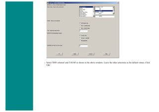
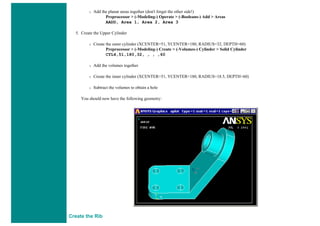
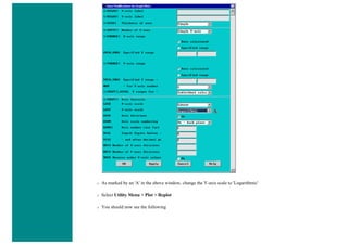
❍ Select Solution > Analysis Type > Analysis Options
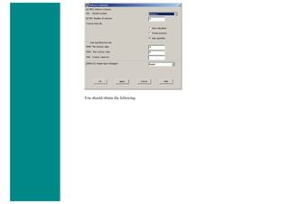
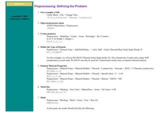
❍ In the following window, change the [SSTIF][PSTRES] item to 'Prestress ON', which ensures the stress stiffness matrix is
calculated. This is required in eigenvalue buckling analysis.](https://image.slidesharecdn.com/univansystutorialsrameesram-240325071613-ff608449/85/Universal-Ansys-Tutorials-Ramees-Ram-pdf-196-320.jpg)
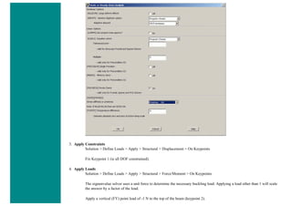
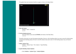
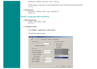

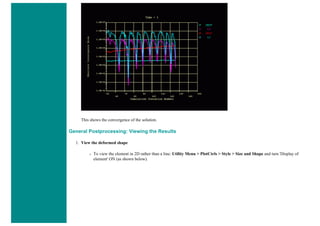

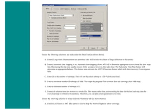
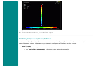
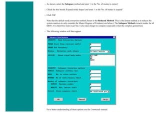
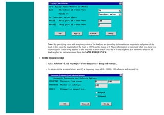
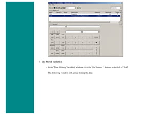
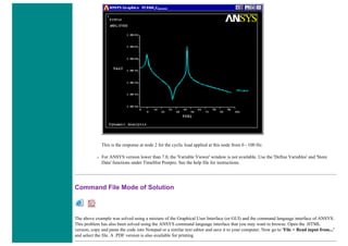

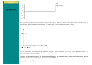

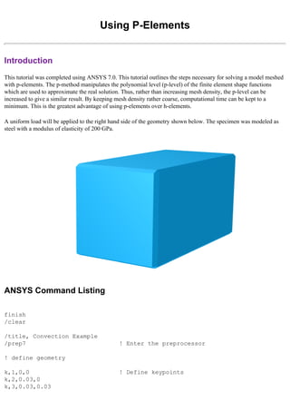
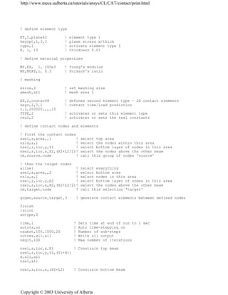
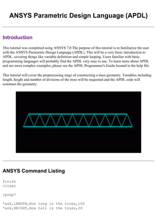
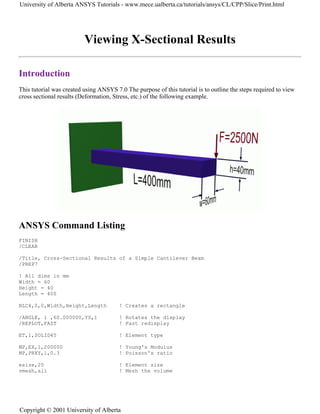
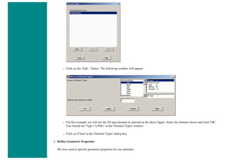
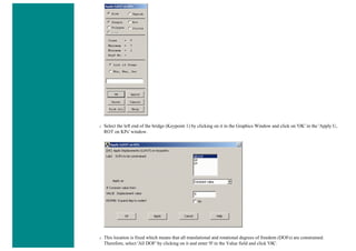
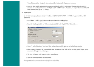
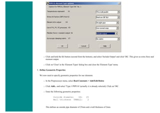
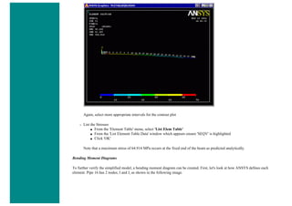
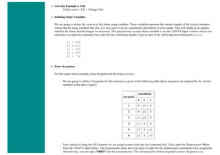
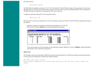
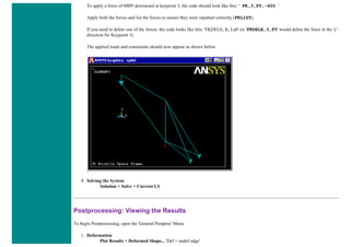
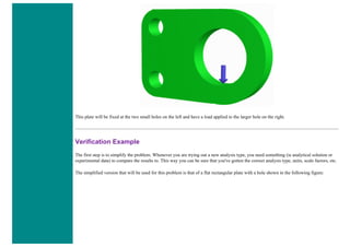
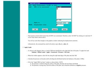
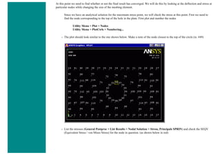
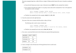
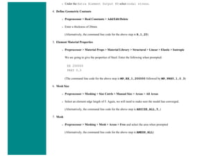
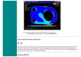
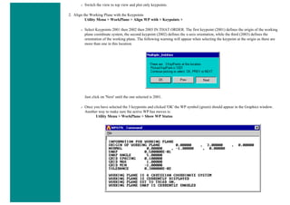
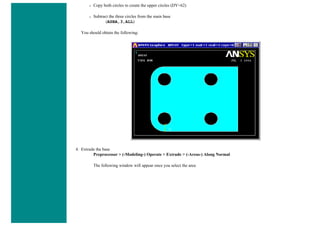
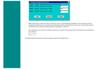
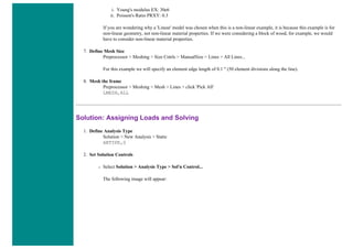
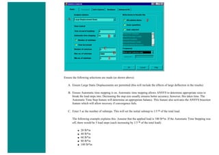
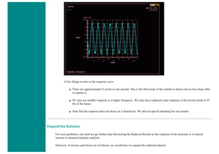
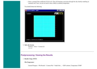
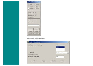
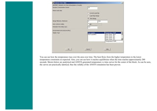
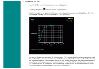
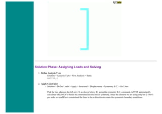
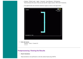
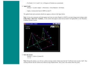
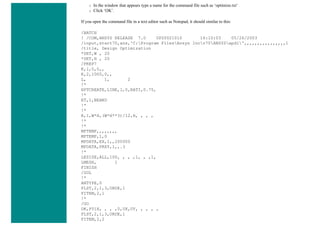
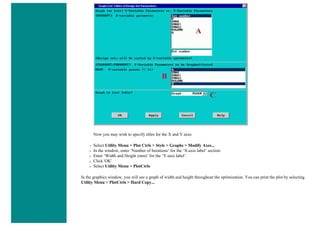
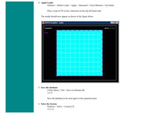
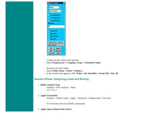
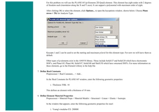
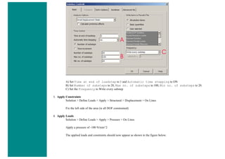
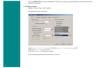
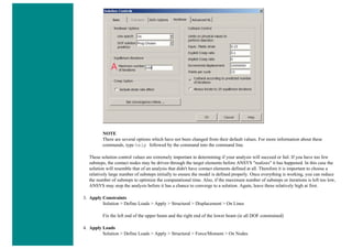
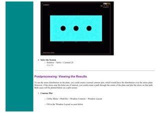
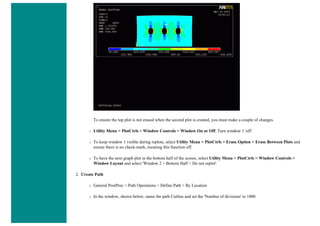
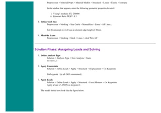
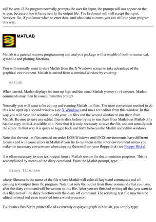
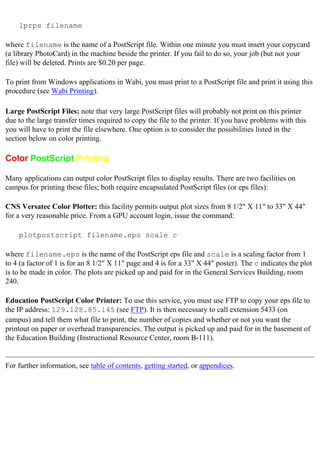
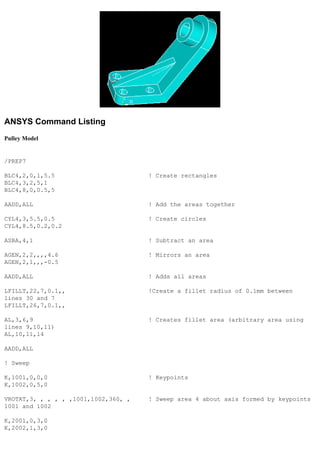
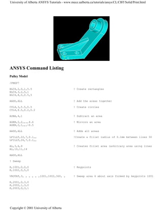
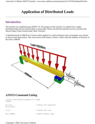
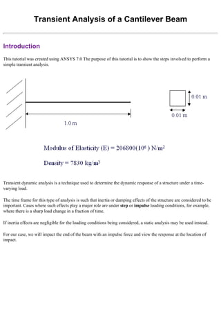
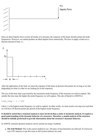
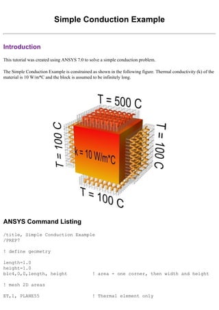
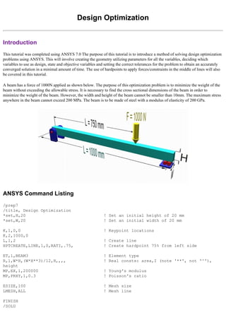
![4. Apply Loads
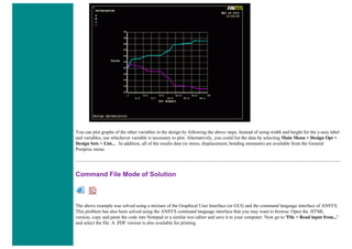
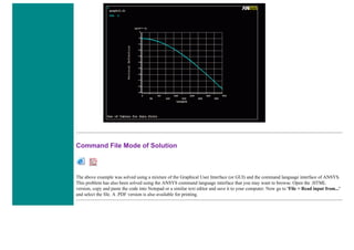
We will define our impulse load using Load Steps. The following time history curve shows our load steps and time steps. Note that
for the reduced method, a constant time step is required throughout the time range.
We can define each load step (load and time at the end of load segment) and save them in a file for future solution purposes. This is
highly recommended especially when we have many load steps and we wish to re-run our solution.
We can also solve for each load step after we define it. We will go ahead and save each load step in a file for later use, at the same
time solve for each load step after we are done defining it.
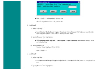
a. Load Step 1 - Initial Conditions
i. Define Load Step
We need to establish initial conditions (the condition at Time = 0). Since the equations for a transient dynamic
analysis are of second order, two sets of initial conditions are required; initial displacement and initial velocity.
However, both default to zero. Therefore, for this example we can skip this step.
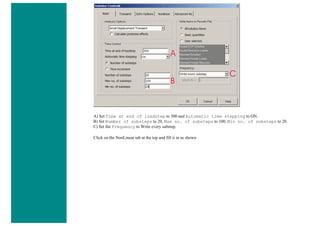
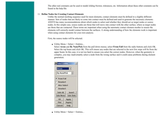
ii. Specify Time and Time Step Options
■ Select Solution > Load Step Opts > Time/Frequenc > Time - Time Step ..
■ set a time of 0 for the end of the load step (as shown below).
■ set [DELTIM] to 0.001. This will specify a time step size of 0.001 seconds to be used for this load
step.](https://image.slidesharecdn.com/univansystutorialsrameesram-240325071613-ff608449/85/Universal-Ansys-Tutorials-Ramees-Ram-pdf-257-320.jpg)


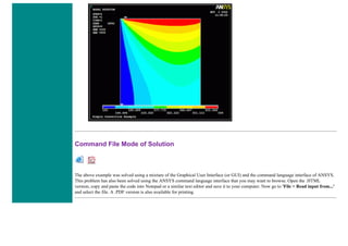


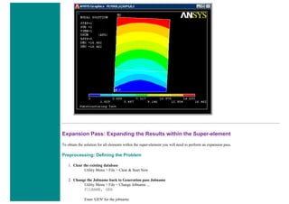
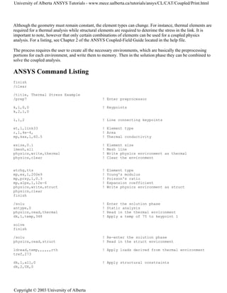
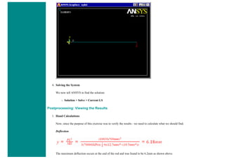
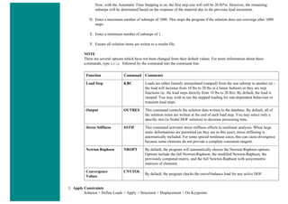
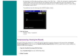
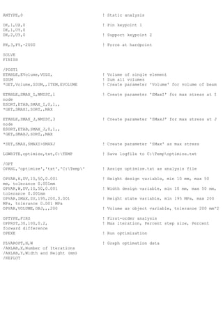
![procedures associated with a particular engineering discipline [will be referred to as] a physics analysis. When the input of one physics
analysis depends on the results from another analysis, the analyses are coupled."
Thus, each different physics environment must be constructed seperately so they can be used to determine the coupled physics solution.
However, it is important to note that a single set of nodes will exist for the entire model. By creating the geometry in the first physical
environment, and using it with any following coupled environments, the geometry is kept constant. For our case, we will create the
geometry in the Thermal Environment, where the thermal effects will be applied.
Although the geometry must remain constant, the element types can change. For instance, thermal elements are required for a thermal
analysis while structural elements are required to deterime the stress in the link. It is important to note, however that only certain
combinations of elements can be used for a coupled physics analysis. For a listing, see Chapter 2 of the ANSYS Coupled-Field Guide
located in the help file.
The process requires the user to create all the necessary environments, which are basically the preprocessing portions for each
environment, and write them to memory. Then in the solution phase they can be combined to solve the coupled analysis.
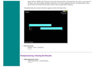
Thermal Environment - Create Geometry and Define Thermal Properties
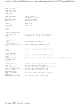
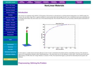
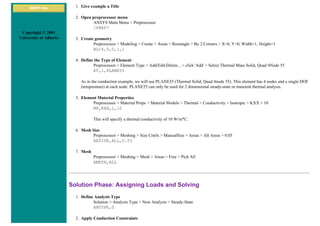
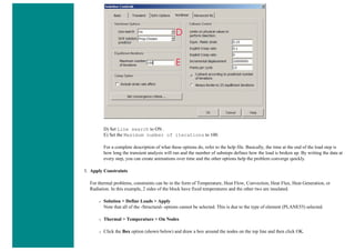
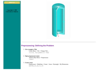
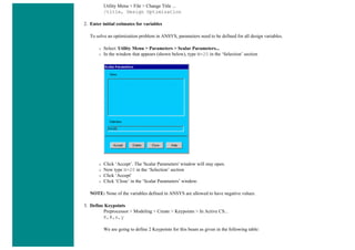
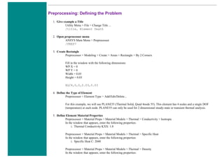
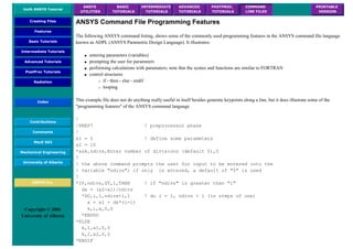
1. Give example a Title
Utility Menu > File > Change Title ...
/title, Thermal Stress Example
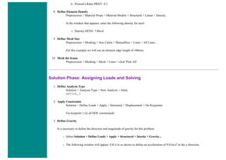
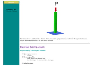
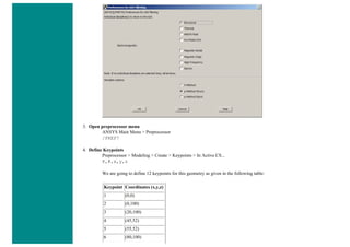
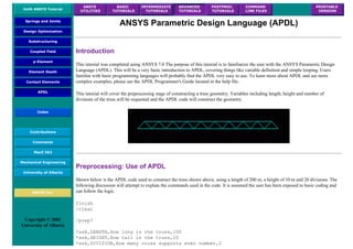
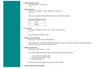
2. Open preprocessor menu
ANSYS Main Menu > Preprocessor
/PREP7
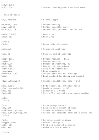
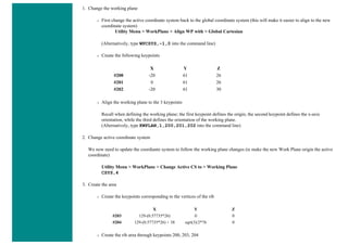
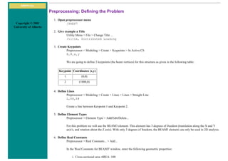
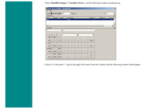
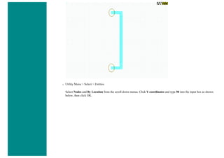
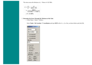
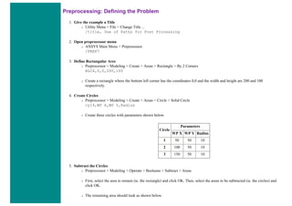
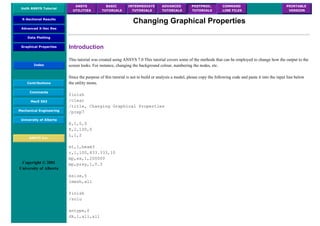
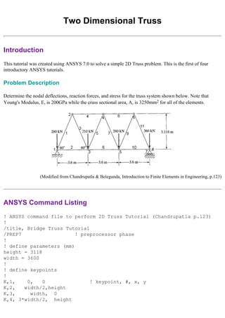
3. Define Keypoints
Preprocessor > Modeling > Create > Keypoints > In Active CS...
K,#,x,y,z
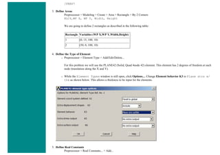
We are going to define 2 keypoints for this link as given in the following table:
Keypoint Coordinates (x,y,z)
1 (0,0)
2 (1,0)
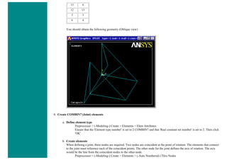
4. Create Lines
Preprocessor > Modeling > Create > Lines > Lines > In Active Coord
L,1,2](https://image.slidesharecdn.com/univansystutorialsrameesram-240325071613-ff608449/85/Universal-Ansys-Tutorials-Ramees-Ram-pdf-359-320.jpg)


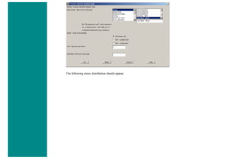

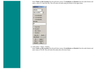
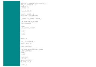

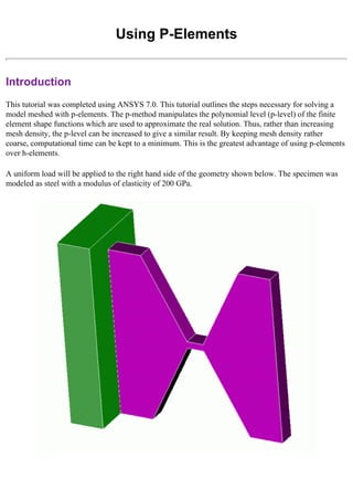
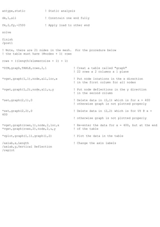
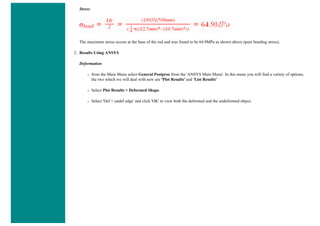
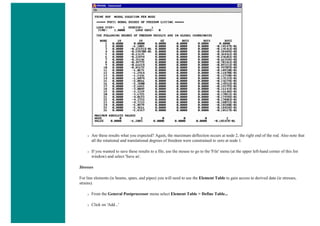
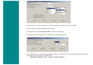
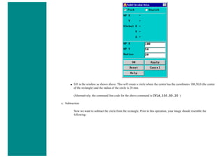
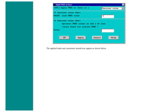
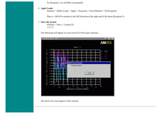
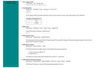
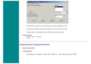
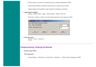
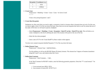
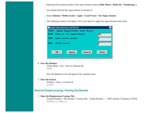
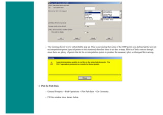
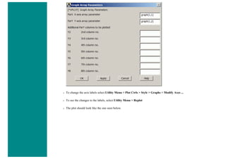
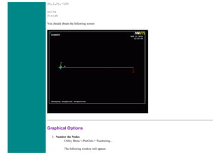
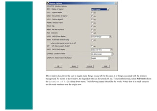
![❍ Fill the next two window in with the following parameters
Parameters
Path Point Number X Loc Y Loc Z Loc
1 0 50 0
2 200 50 0
When the third window pops up, click 'Cancle' because we only enabled two points on the path in the previous step.
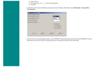
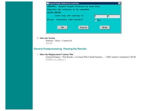
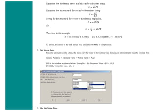
3. Map the Stress onto the Path
Now the path is defined, you must choose what to map to the path, or in other words, what results should be available to the
path. For this example, equivalent stress is desired.
❍ General Postproc > Path Operations > Map onto Path
❍ Fill the next window in as shown below [Stress > von Mises] and click OK.](https://image.slidesharecdn.com/univansystutorialsrameesram-240325071613-ff608449/85/Universal-Ansys-Tutorials-Ramees-Ram-pdf-433-320.jpg)
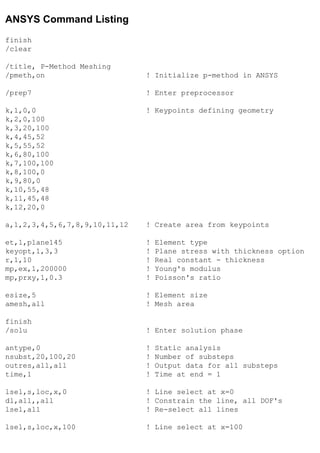
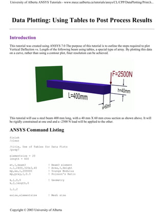
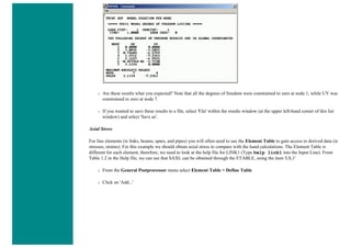
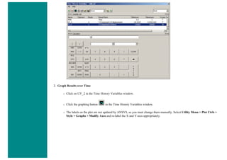
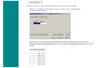
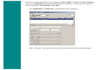
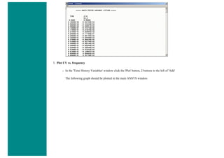
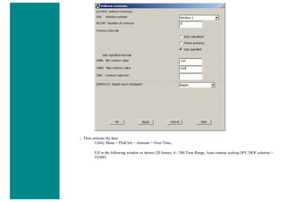
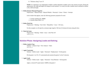
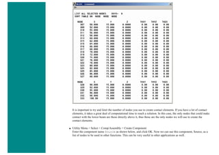
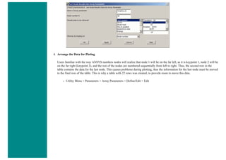
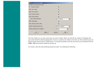
![❍ Utility Menu > Parameters > Array Parameters > Define/Edit > Add
❍ The window seen above will pop up. Fill it out as shown [Graph > Table > 22,2,1]. Note there are 22 rows, one more than
the number of nodes. The reason for this will be explained below. Click OK and then close the 'Define/Edit' window.
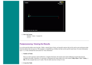
3. Enter Data into Table
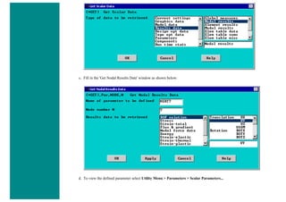
First, the horizontal location of the nodes will be recorded
❍ Utility Menu > Parameters > Get Array Data ...
❍ In the window shown below, select Model Data > Nodes](https://image.slidesharecdn.com/univansystutorialsrameesram-240325071613-ff608449/85/Universal-Ansys-Tutorials-Ramees-Ram-pdf-441-320.jpg)
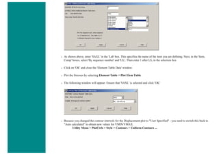
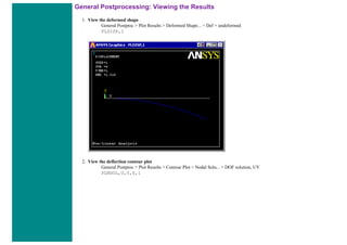
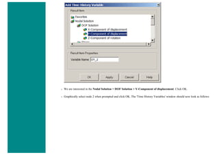
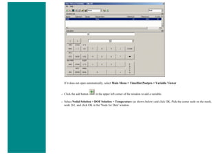
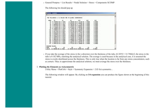
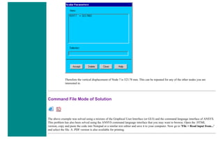
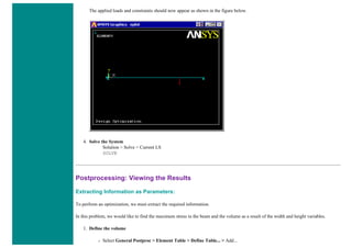
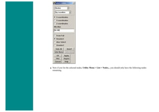
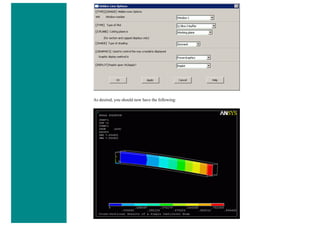
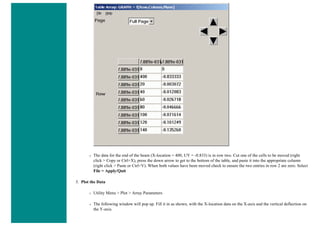
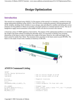
![❍ Fill the next window in as shown below and click OK [Graph(1,1) > All > Location > X]. Naming the array parameter
'Graph(1,1)' fills in the table starting in row 1, column 1, and continues down the column.
Next, the vertical displacement will be recorded.
❍ Utility Menu > Parameters > Get Array Data ... > Results data > Nodal results
❍ Fill the next window in as shown below and click OK [Graph(1,2) > All > DOF solution > UY]. Naming the array
parameter 'Graph(1,2)' fills in the table starting in row 1, column 2, and continues down the column.](https://image.slidesharecdn.com/univansystutorialsrameesram-240325071613-ff608449/85/Universal-Ansys-Tutorials-Ramees-Ram-pdf-442-320.jpg)
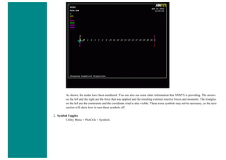
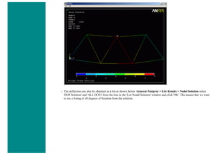
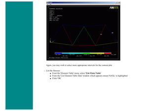
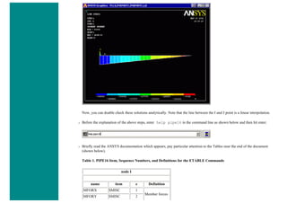
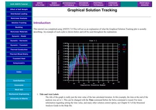
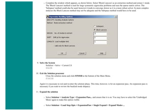
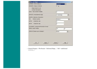
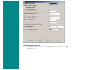
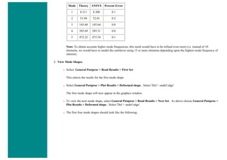
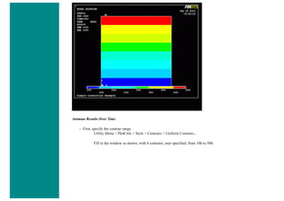
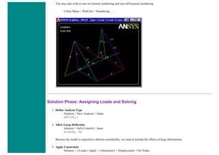
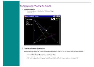
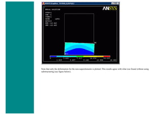
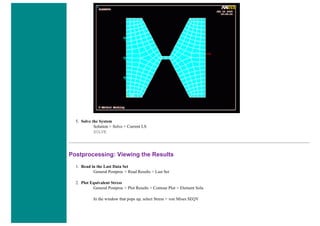
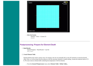
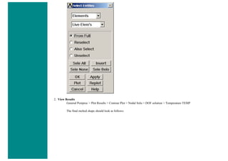
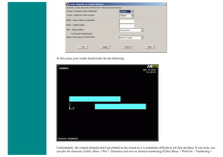
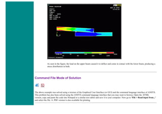
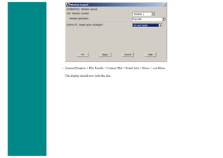
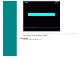
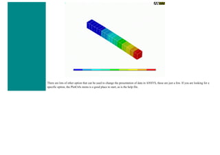
![When using line elements, such as BEAM3, it is sometime difficult to visualize what the elements really look like. To aid in
this process, ANSYS can display the elements shapes based on the real constant description. Click on the toggle box beside
[/ESHAPE] to turn on element shapes and click OK to close the window.
If there is no change in output, don't be alarmed. Recall we selected a plot of just the nodes, thus elements are not going to
show up. Select Utility Menu > Plot > Elements. The following should appear.](https://image.slidesharecdn.com/univansystutorialsrameesram-240325071613-ff608449/85/Universal-Ansys-Tutorials-Ramees-Ram-pdf-455-320.jpg)
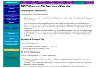


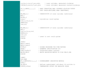
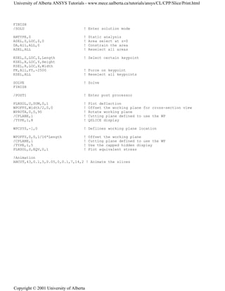
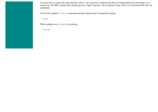
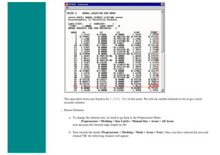
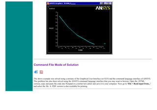
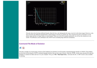
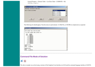
![FORTRAN
The FORTRAN compiler is invoked by typing:
xlf [-options] filename.f
Normally no options are required. For learning about the compiler's many options, type the
command, xlf by itself. If your program code consists of many files and libraries, consider using a
make file to simplify the program's maintenance.
Note that the name of the FORTRAN program must have an extension of lower case 'f'; i.e. your file
must be named something like test.f and not test.for or TEST.F. If you compile a program
using the syntax xlf test.f, the name of the resulting executable will default to a.out (logical,
isn't it?). This program would be run by entering ./a.out. To change the executable's output name
to test, for example, we would compile the program in the following way:
xlf -o test test.f
To run this program, you now type, ./test. Note that the ./ preceding the name of the executable
can be omitted if the current directory '.' is in your path (this is changed in your .cshrc file; see
Configuration Files).
It is possible (and usually desirable) to have source code in multiple files. For example you might
have a main program and several subroutine files. These can be compiled and linked in one-step by:
xlf -o main main.f sub1.f sub2.f sub3.f
Sending compiler error messages to a file: If you want to send the compiler output, such as error
messages, to a file, you can do it by appending >& errorfile to the xlf command line. For
example:
xlf main.f sub1.f >& errorfile
will compile main.f and sub1.f and send any compiler output to the file errorfile.
Capturing program output: To send output from a program to a file instead of the screen (i.
e. redirecting it), execute the program as follows:
test > output
where test is the name of the executable, and output is the name of the file to which the output](https://image.slidesharecdn.com/univansystutorialsrameesram-240325071613-ff608449/85/Universal-Ansys-Tutorials-Ramees-Ram-pdf-485-320.jpg)


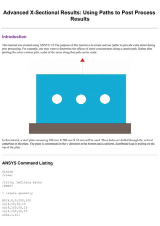
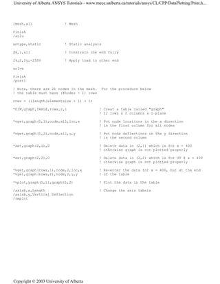
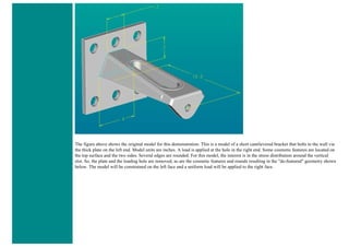
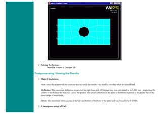
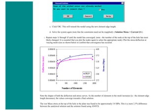
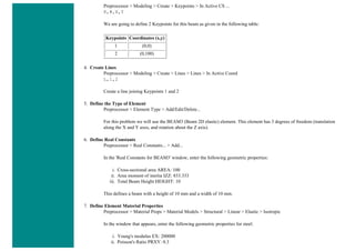
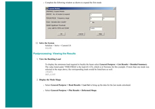
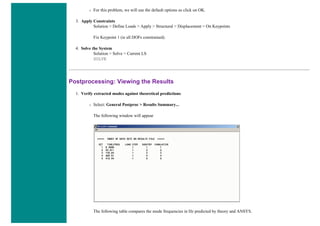
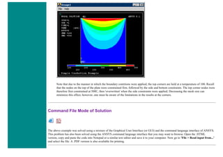
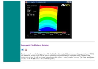
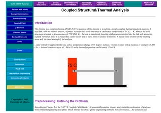
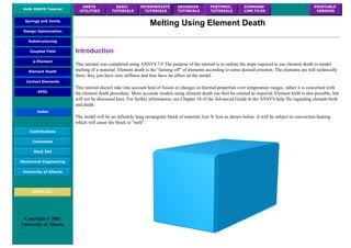
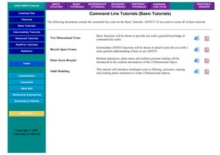
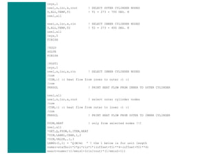
![Coupled Structural/Thermal Analysis
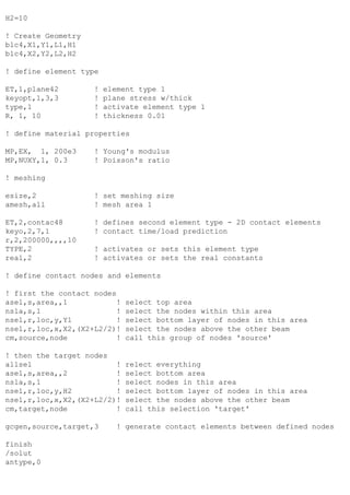
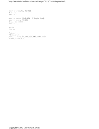
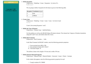
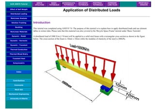
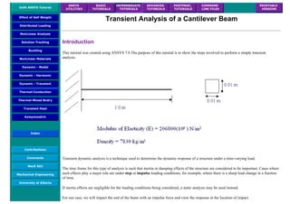
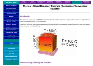
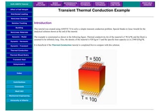
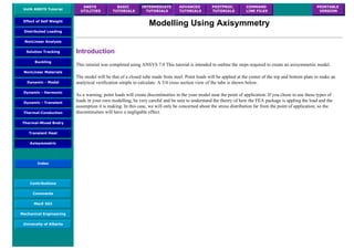
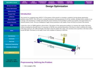
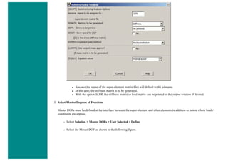
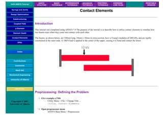
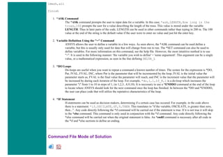
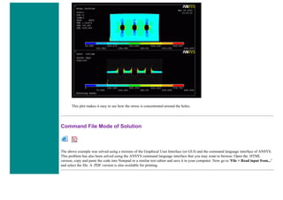
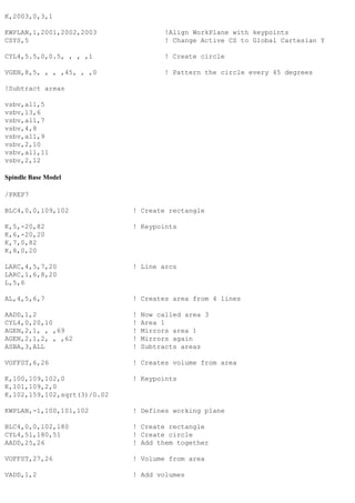
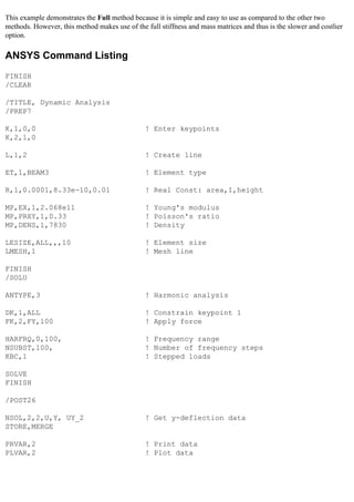
Introduction
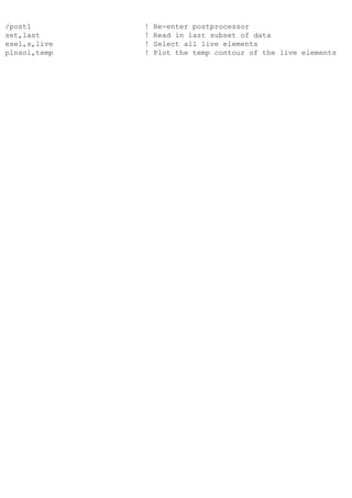
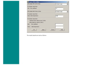
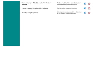
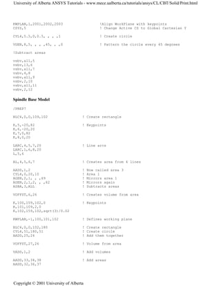
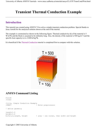
This tutorial was completed using ANSYS 7.0 The purpose of this tutorial is to outline a simple coupled thermal/structural
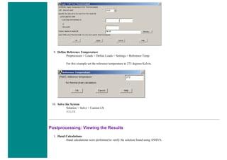
analysis. A steel link, with no internal stresses, is pinned between two solid structures at a reference temperature of 0 C (273
K). One of the solid structures is heated to a temperature of 75 C (348 K). As heat is transferred from the solid structure into
the link, the link will attemp to expand. However, since it is pinned this cannot occur and as such, stress is created in the
link. A steady-state solution of the resulting stress will be found to simplify the analysis.
Loads will not be applied to the link, only a temperature change of 75 degrees Celsius. The link is steel with a modulus of
elasticity of 200 GPa, a thermal conductivity of 60.5 W/m*K and a thermal expansion coefficient of 12e-6 /K.
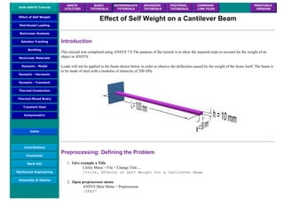
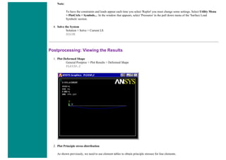
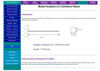
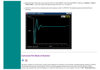
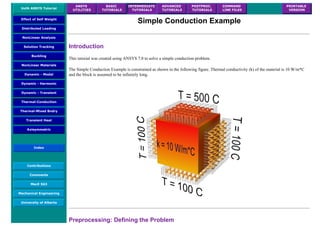
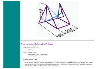
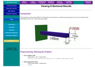
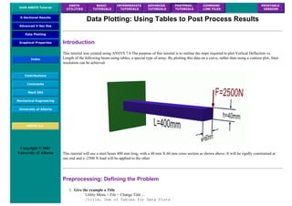
Preprocessing: Defining the Problem
According to Chapter 2 of the ANSYS Coupled-Field Guide, "A sequentially coupled physics analysis is the combination
of analyses from different engineering disciplines which interact to solve a global engineering problem. For convenience, ...
the solutions and procedures associated with a particular engineering discipline [will be referred to as] a physics analysis.
When the input of one physics analysis depends on the results from another analysis, the analyses are coupled."
Thus, each different physics environment must be constructed seperately so they can be used to determine the coupled
physics solution. However, it is important to note that a single set of nodes will exist for the entire model. By creating the
geometry in the first physical environment, and using it with any following coupled environments, the geometry is kept
constant. For our case, we will create the geometry in the Thermal Environment, where the thermal effects will be applied.
Although the geometry must remain constant, the element types can change. For instance, thermal elements are required for
a thermal analysis while structural elements are required to deterime the stress in the link. It is important to note, however
that only certain combinations of elements can be used for a coupled physics analysis. For a listing, see Chapter 2 of the
ANSYS Coupled-Field Guide located in the help file.
The process requires the user to create all the necessary environments, which are basically the preprocessing portions for
each environment, and write them to memory. Then in the solution phase they can be combined to solve the coupled](https://image.slidesharecdn.com/univansystutorialsrameesram-240325071613-ff608449/85/Universal-Ansys-Tutorials-Ramees-Ram-pdf-601-320.jpg)

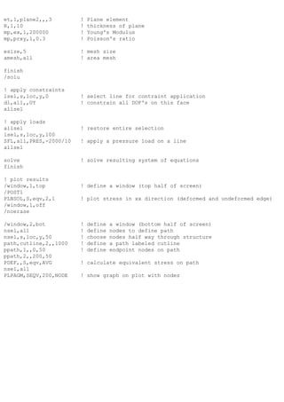
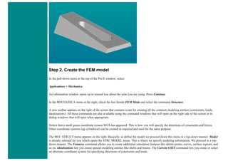
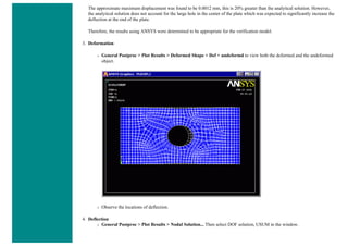
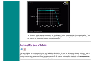
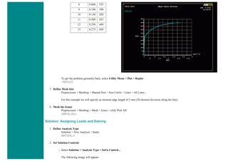
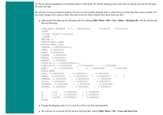
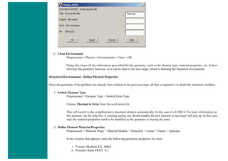
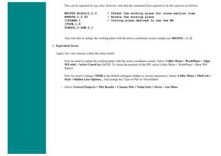
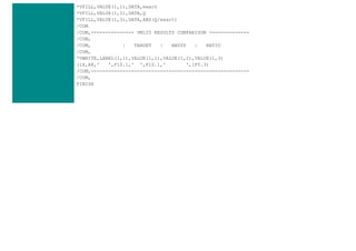
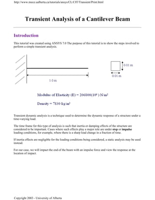
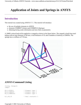
![Coupled Structural/Thermal Analysis
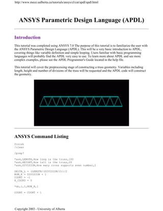
Introduction
This tutorial was completed using ANSYS 7.0 The purpose of this tutorial is to outline a simple coupled
thermal/structural analysis. A steel link, with no internal stresses, is pinned between two solid structures at a
reference temperature of 0 C (273 K). One of the solid structures is heated to a temperature of 75 C (348 K). As
heat is transferred from the solid structure into the link, the link will attemp to expand. However, since it is
pinned this cannot occur and as such, stress is created in the link. A steady-state solution of the resulting stress
will be found to simplify the analysis.
Loads will not be applied to the link, only a temperature change of 75 degrees Celsius. The link is steel with a
modulus of elasticity of 200 GPa, a thermal conductivity of 60.5 W/m*K and a thermal expansion coefficient of
12e-6 /K.
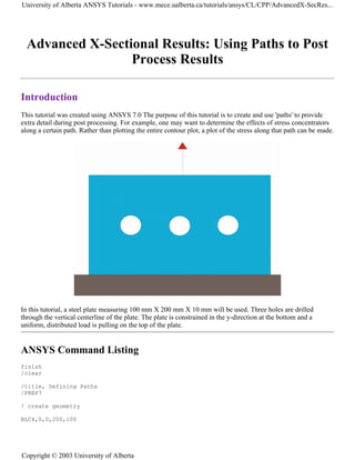
Preprocessing: Defining the Problem
According to Chapter 2 of the ANSYS Coupled-Field Guide, "A sequentially coupled physics analysis is the
combination of analyses from different engineering disciplines which interact to solve a global engineering
problem. For convenience, ...the solutions and procedures associated with a particular engineering discipline
[will be referred to as] a physics analysis. When the input of one physics analysis depends on the results from
another analysis, the analyses are coupled."
Thus, each different physics environment must be constructed seperately so they can be used to determine the
coupled physics solution. However, it is important to note that a single set of nodes will exist for the entire
model. By creating the geometry in the first physical environment, and using it with any following coupled
environments, the geometry is kept constant. For our case, we will create the geometry in the Thermal
Environment, where the thermal effects will be applied.
University of Alberta ANSYS Tutorials - www.mece.ualberta.ca/tutorials/ansys/CL/CAT/Coupled/Print.html
Copyright © 2003 University of Alberta](https://image.slidesharecdn.com/univansystutorialsrameesram-240325071613-ff608449/85/Universal-Ansys-Tutorials-Ramees-Ram-pdf-604-320.jpg)