UNIT – 5 NLP • Perception/Action • Machine Learning 1. Complexity of the Problem (Language Problems) Natural language is difficult for computers because of the following reasons: 1. Ambiguity: A single word or sentence may have multiple meanings. Example: “Bank” = river bank / financial bank. 2. Synonyms: Different words may have similar meanings. Example: big, huge, large. 3. Grammar Rules: Languages have complex and irregular grammar structures. 4. Context Understanding: Meaning changes depending on the situation. Example: “He is cold” → temperature OR behavior? Because of these problems, computers find it hard to interpret human language accurately. 2. Natural Language Processing (NLP) Stages NLP converts human language into a form machines can understand. It works in three main levels: (a) Syntactic Processing (Structure / Grammar Level) Deals with how words form sentences. Includes: • Sentence structure analysis • Phrase detection (NP, VP) • POS Tagging (noun, verb, adjective, etc.) Example: “The dog runs fast.” POS = (Det, Noun, Verb, Adv) (b) Semantic Analysis (Meaning Level) Extracts actual meaning of words and relations. Includes: • Word meanings • Synonyms • Semantic roles (who did what) Example: “Ram ate an apple.” Ram = agent Apple = object (c) Pragmatic Processing (Context Level) Interprets intended meaning, not literal words. Example: “Can you pass the salt?” Not asking about ability → It is a request. Pragmatics = real-world meaning using context. 3. Perception & Action (Robotics Context) Robotic systems need to sense and act. (a) Perception • Collecting information from the environment. • Done using sensors: o Cameras o Microphones o Touch sensors o Lidar Goal: Convert raw sensor data → useful understanding. Example: Detecting obstacles using camera or lidar. (b) Action • Acting based on perception. • Uses actuators: o Motors o Wheels o Arms o Grippers Example: Robot sees an object → picks it up. Perception + Action = Intelligent Robot Behavior 4. Machine Learning Machine learning allows systems to learn patterns from data. It has two main tasks: 1. Clustering 2. Classification 4.1 Clustering (Unsupervised Learning) Clustering groups similar data points together. A. Standard K-Means (Lloyd Algorithm) Steps: 1. Select k initial cluster centers. 2. Assign each point to the nearest center. 3. Update centers (mean of assigned points). 4. Repeat until centers do not change. Advantages: • Simple • Fast Disadvantages: • Depends on initial choice of centers • Stuck in local minima B. Generalized Clustering Techniques Used when data is more complex. 1. Over-Partitioning • K-means may create more clusters than necessary. • Leads to incorrect grouping. 2. Merging • Combines similar clusters when they are too close. C. Modifications of K-Means 1. Better Initialization Techniques • K-Means++ • Random multiple restarts 2. Avoid Local Minima • Use different starting points • Use K-harmonic means 3. Faster Update Methods • Use efficient distance

1. MODEL FITTING
UNIT-2

2. INTRODUCTION
• Model Fitting: Hough Transform, Line Fitting, Ellipse and Conic
Sections Fitting, Algebraic and Euclidean Distance Measures
• Camera Calibration: Camera Models, Intrinsic and Extrinsic
Parameters, Radial Lens Distortion, Direct Parameter Calibration,
Camera Parameters from Projection Matrices, Orthographic, Weak
Perspective, Affine, and Perspective Camera Models
• Epipolar Geometry: Introduction to Projective Geometry, Epipolar
Constraints, The Essential and Fundamental Matrices, Estimation of
the Essential/Fundamental Matrix

3. Hough Transform
• The Hough Transform is a feature-extraction method used to detect
geometric shapes like lines, circles, and ellipses in images.
• The key idea is to map points in the image (spatial domain) into a
parameter space (sometimes called accumulator space), where each
point votes for possible shape parameters.
• Peaks in that parameter space indicate candidate shapes — because
many image points “agree” on the same parameters.
• For line detection, the parametric form used is:
ρ=xcos⁡
θ+ysin⁡
θ
where ρ is the distance from origin to the line, and θ is the line’s angle

4. Hough Transform
• Each edge point (x,y) in the image gives a sinusoidal curve in (ρ,θ)
space. An intersection (a “vote peak”) suggests a line.
• Variants:
⚬ Standard Hough Transform (SHT): votes over all parameter
combinations.
⚬ Probabilistic Hough Transform (PHT): samples a subset of edge
points to reduce computation.
⚬ Generalized Hough Transform (GHT): matches templates to
detect arbitrary shapes, not just simple one.

6. Line Fitting
• Line fitting is the process of finding the best line that represents a set
of points in an image or dataset.
• Unlike the Hough Transform (which votes in parameter space), line
fitting directly estimates the line equation from data points.
• The common goal is to minimize the error between the actual data
points and the fitted line.
• Used in tasks like edge detection, boundary approximation, and object
recognition.

7. Methods of Line Fitting
• Least Squares Fitting: Finds a line by minimizing the sum of squared
distances of points to the line.
• Algebraic Distance: Measures the error based on the equation of the
line; simpler but less accurate.
• Euclidean Distance: Measures the shortest perpendicular distance of
each point to the line; more precise but computationally heavier.
• Applications include motion tracking, image segmentation, and
detecting geometric patterns in images.

8. Ellipse and Conic Sections Fitting
• Conic sections (lines, circles, ellipses, parabolas, hyperbolas) can be
represented by the general quadratic equation:
Ax^2+Bxy+Cy^2+Dx+Ey+F=0
• Fitting means finding the parametersA,B,C,D,E,F that best describe
the curve passing through or near a given set of data points.
• Ellipse fitting is a common task in computer vision for detecting
circular or oval shapes in noisy images
• Different fitting methods balance accuracy, speed, and robustness
to noise, depending on the application.

9. Methods for Fitting Conics
• Algebraic Fitting: Minimizes the error in the conic equation itself;
faster but less accurate.
• Geometric (Euclidean) Fitting: Minimizes the actual distance
between points and the conic curve; more precise but
computationally expensive.
• Constraints (such as B^2 - 4AC < 0 for ellipses) are applied to
ensure the correct type of conic is fitted.
• Applications: iris recognition, cell shape detection in medical
images, and object boundary approximation.

10. Algebraic Distance Measures
• The algebraic distance is a simple way to evaluate how well a point
(x,y) satisfies the equation of a line, ellipse, or other curve.
• For a general conic Ax^2 + Bxy + Cy^2 + Dx + Ey + F = 0, the
algebraic distance is just the value of the equation when (x,y) is
substituted.
• Advantage: Easy to compute, suitable for fast fitting.
• Limitation: Does not represent the true geometric distance, so
accuracy may be low for noisy data.

11. Euclidean Distance Measures
• The Euclidean distance measures the shortest perpendicular
distance between a point and the fitted shape.
• For a line ax+by+c=0, the Euclidean distance of a point (x0,y0) is:
• Advantage: Represents the true error, giving more accurate fitting
results.
• Limitation: Computationally more expensive compared to
algebraic distance.

12. Camera Calibration
• Camera calibration is the process of estimating the parameters of a
camera to relate 3D world coordinates to 2D image coordinates.
• It corrects image distortions and provides accurate measurements for
computer vision tasks.
• Parameters are divided into:
⚬ Intrinsic parameters: internal camera properties such as focal
length, principal point, skew, and lens distortion.
⚬ Extrinsic parameters: position and orientation of the camera with
respect to the world.
• Calibration is essential for 3D reconstruction, robot navigation, and
augmented reality.

14. Camera Models
• A camera model is a mathematical representation of how a camera
captures the 3D world and projects it onto a 2D image. In simpler terms,
it describes how points in the real world (3D) are transformed into points
on an image (2D).
• Camera models are essential in computer vision for tasks like 3D
reconstruction, object tracking, and camera calibration, because they
allow us to understand the relationship between the physical world and
the images we capture.
• A camera model typically considers:
⚬ Intrinsic parameters – internal properties of the camera like focal
length, optical center (principal point), and lens distortion.

15. Types Of Camera Models
• Pinhole Camera Model: Simplest camera model. Assumes light passes
through a single point (the pinhole) and projects onto a flat image
plane.
Characteristics: No lens distortion, idealized model.
Use: Fundamental for computer vision theory and calibration.
• Lens (or Perspective) Camera Model: Real cameras have lenses; this
model extends the pinhole model to include effects of lenses.
Characteristics: model perspective projection with intrinsic parameters.
Use: More accurate modeling for real-world cameras.
• Orthographic Camera Model: Assumes rays from the object are
parallel rather than converging to a point.

16. Types Of Camera Models
• Weak Perspective Camera Model: Approximation between pinhole
and orthographic models. Assumes objects are far from the camera
relative to depth variations.
Characteristics: Simplifies perspective projection.
Use: Common in face alignment and 3D shape estimation.
• Fish-eye / Wide-angle Camera Model: Models cameras with ultra-
wide lenses that cause strong distortion.
Characteristics: Non-linear distortion, can capture a very wide field of
view.
Use: Panoramic imaging, robotics, autonomous vehicles.

17. Radial Lens Distortion
• Radial lens distortion occurs due to the shape of the camera lens,
causing straight lines to appear curved in the image.
• It is more pronounced near the edges of the image.
• Types of radial distortion:
⚬ Barrel Distortion: Lines bulge outwards (like a barrel).
⚬ Pincushion Distortion: Lines bend inwards (like a pincushion).
• Common in wide-angle lenses.

19. Radial Lens Distortion
Radial distortion can be modeled mathematically:
• r Distance from image center
→
• k1,k2,k3 Distortion coefficients
→
• Correction: Reverse the distortion using calibration techniques.
• Used in photogrammetry, computer vision, and camera calibration.

20. Direct Parameter Calibration
• Direct Parameter Calibration is a process used to estimate the
camera’s intrinsic and extrinsic parameters directly from a set of
known 3D–2D point correspondences.
• The goal is to find parameters that minimize the difference
between the observed image points and the projected points from
the 3D world.
• It eliminates intermediate steps by directly solving the camera
projection equations.
• This method is often used when precise calibration patterns (like
checkerboards) and accurate measurements are available.

21. Direct Parameter Calibration
Steps involved:
• Capture several images of a known calibration pattern (like a grid or
checkerboard).
• Identify matching points between the 3D object and the 2D image.
• Use mathematical optimization to minimize projection error and
estimate intrinsic and extrinsic parameters.
Importance:
• Produces highly accurate calibration results.
• Reduces distortion and improves 3D reconstruction accuracy.
• Commonly used in robotics, stereo vision, and camera-based
measurement systems.

22. Camera Parameters from Projection Matrices
• The projection matrix defines how a 3D point in the world is mapped
onto a 2D image point in the camera.
• It combines both intrinsic and extrinsic parameters of the camera into
a single 3×4 matrix P.
• The general form of the projection equation is:
where (X,Y,Z) are 3D world coordinates and ((x,y) are image coordinates.
• The scale factor s accounts for homogeneous coordinates.

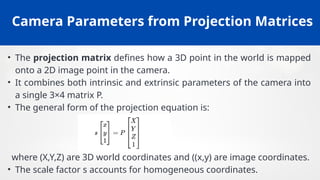
23. Extracting Camera Parameters from Projection
Matrix
• The projection matrix P can be decomposed as:
P=K[R t]
∣
where:
⚬ K = intrinsic parameter matrix (focal length, principal point, skew).
⚬ R = rotation matrix (orientation of camera).
⚬ t= translation vector (camera position).
• Decomposition allows us to find both internal characteristics of the
camera and its position/orientation in the world.
• This approach is fundamental for 3D reconstruction, stereo calibration,
and motion tracking.

24. Orthographic Camera Model
• The Orthographic Camera Model is the simplest type of projection
used in computer vision.
• It assumes that all projection lines from 3D points to the image
plane are parallel to each other and perpendicular to the image
plane.
• Depth information is ignored, meaning that objects at different
distances appear the same size.
• This model is useful for analyzing small, flat objects or when the
camera is placed far from the scene.

25. Orthographic Camera Model
• The orthographic projection of a 3D point (X,Y,Z) to a 2D image point (x,y)
is given by:
x=X,y=Y
or in matrix form:
• Key features:
⚬ Preserves shape and size of objects.
⚬ Does not provide depth perception.
⚬ Commonly used in engineering drawings and object measurement
tasks.

26. Weak Perspective
• The Weak Perspective Camera Model is an approximation of the
full perspective projection.
• It assumes that the object being viewed is small compared to its
distance from the camera, so all points are roughly at the same
depth.
• In this model, the projection lines are nearly parallel, which
simplifies the mathematics while still maintaining some
perspective effects.
• It provides a balance between the simplicity of the affine model
and the accuracy of the full perspective model.

27. Weak Perspective
• The projection of a 3D point (X,Y,Z) onto a 2D image point (x,y) is
given by:
x=sX,y=s
where s=f / Zavgs and Zavg​is the average depth of the object.
• Key characteristics:
⚬ Maintains scale consistency for objects at similar depths.
⚬ Simplifies computations in motion analysis and shape recovery.
⚬ Used in applications like facial modeling and 3D pose
estimation.

28. Affine Camera Model
• The Affine Camera Model is an approximation of the Perspective
Camera Model, used when the depth variation of the object is
small compared to its distance from the camera.
• It assumes that projection rays are nearly parallel, making it easier
to perform linear calculations.
• The affine model preserves parallelism between lines but not
angles or lengths.
• It is widely used in tasks like motion estimation, shape analysis,
and 3D object recognition when high accuracy of depth is not
required.

29. Affine Camera Model
• The affine projection of a 3D point (X,Y,Z) to a 2D point (x,y) is given
by:
where A is a 2×3 affine transformation matrix and t is a translation
vector.
• Key features:
⚬ Linear transformation simplifies computation.
⚬ Suitable for planar scenes or distant objects.

30. Perspective Camera Models
• The Perspective Camera Model is a mathematical representation of
how a real camera captures the 3D world onto a 2D image.
• It simulates what our eyes see: objects farther from the camera
appear smaller, and closer objects appear larger.
• It accurately represents depth and foreshortening, making the
images realistic.
• The perspective camera model is essential for any computer vision
task that requires accurate representation of 3D scenes on a 2D
plane.
• Applications: Widely used in 3D reconstruction, photogrammetry,

31. Features - Perspective Camera Models
• Converging Projection Rays: All rays from the 3D points pass
through a single point called the camera center, creating
perspective effects.
• Intrinsic Parameters: Include focal length, principal point, and
skew; these define the internal characteristics of the camera.
• Extrinsic Parameters: Include rotation and translation, which
define the camera’s position and orientation in the world.
• Preserves Angles and Perspective: Unlike affine models, it
accurately models foreshortening and depth variation.

32. Epipolar Geometry
• Epipolar geometry explains the geometric relationship between two
different views of the same 3D scene.
• The line connecting the two camera centers intersects each image
plane at a point called the epipole.
• For any point in one image, the matching point in the second image
must lie on the epipolar line.
• This reduces the correspondence search from a 2D area to a 1D line,
making point matching more efficient.
• Epipolar geometry is fundamental for stereo vision, structure-from-
motion, and 3D reconstruction.

34. Epipolar Constraints
• Epipolar constraint defines the relationship between
corresponding points in two stereo images.
• A point in one image must always lie on the corresponding
epipolar line in the other image.
• This geometric condition significantly reduces the search space for
matching points.
• The constraint ensures correct triangulation for reconstructing 3D
points.
• It provides the mathematical foundation for estimating the
essential and fundamental matrices.

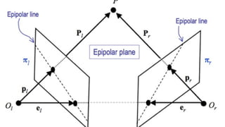
35. The Essential Matrix
• The essential matrix encodes the epipolar geometry between two
calibrated cameras.
• It is defined as E = [t]ₓ R, where R is the relative rotation and t is the
relative translation between cameras.
• The essential matrix relates normalized image coordinates of
corresponding points in the two views.
• It has special properties: it is a rank 2 matrix with singular values of
the form (σ, σ, 0).
• Decomposition of the essential matrix allows recovery of the
relative camera motion (rotation and translation).

36. The Fundamental Matrix
• The fundamental matrix encodes the epipolar geometry between
two uncalibrated cameras.
• It relates pixel coordinates of corresponding points in stereo
images through the equation x′ᵀ F x = 0.
• The matrix has 7 degrees of freedom and is always of rank 2.
• Unlike the essential matrix, it does not require camera calibration.
• It depends only on the relative camera setup and not on the 3D
scene structure.

37. Estimation of the Essential/Fundamental Matrix
• Detect Feature Points: Identify corresponding points in the two
images using methods like SIFT, SURF, or ORB.
• Normalize Points: Improve numerical stability by scaling
coordinates.
• Solve for F or E:
⚬ Use 8-point algorithm (or 7-point algorithm for F) to compute the
matrix.
• Enforce Rank Constraints:
⚬ Fundamental Matrix F must have rank 2.
⚬ Essential Matrix E must have two equal singular values and one

38. THANK YOU