Downloaded 81 times
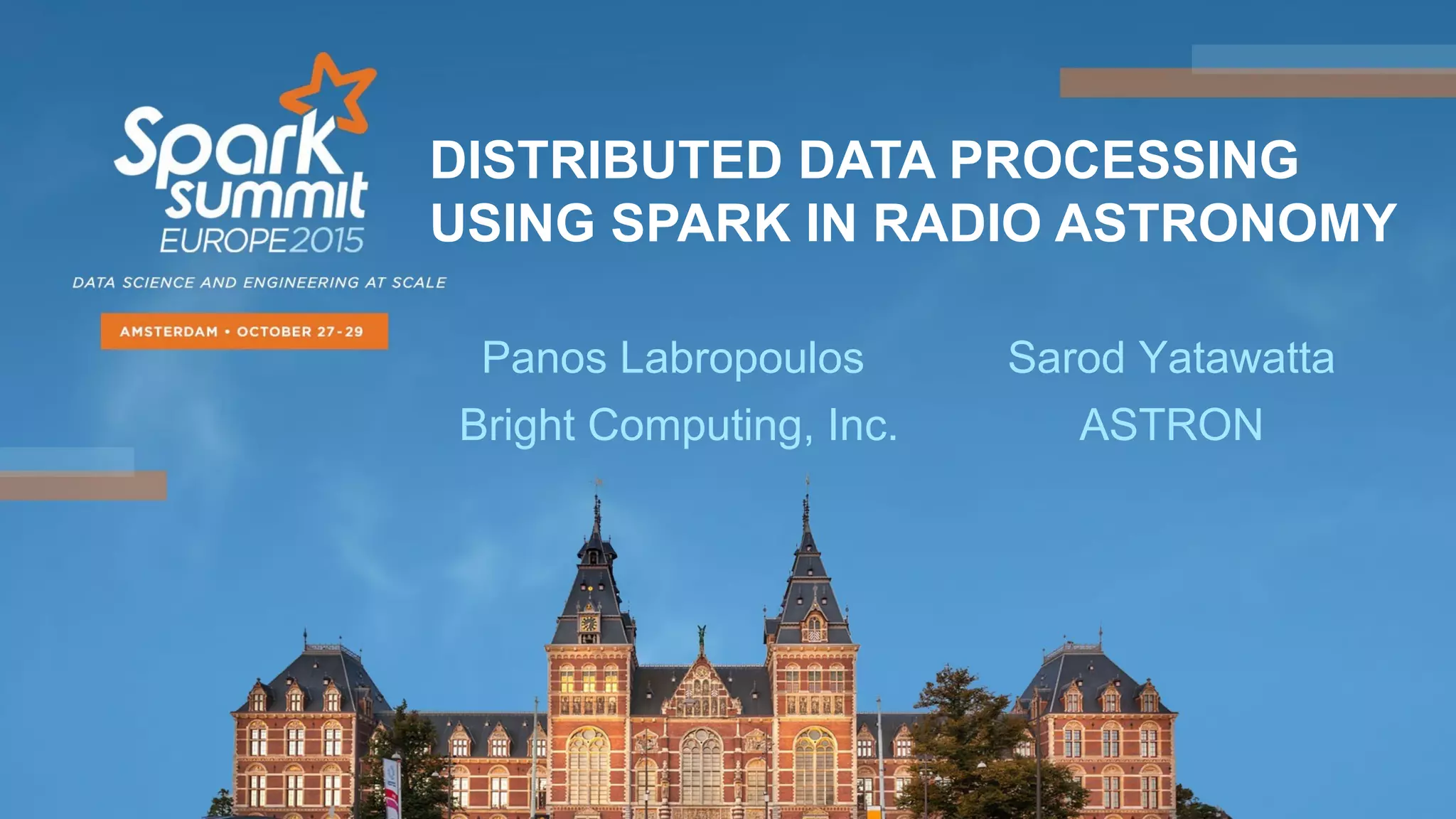

![Measurement process
x
s s
b
cg /sb⋅=τ
)(cos2 tEV ω=])(cos[1 gtEV τω −=
])2(cos)([cos gg tP ωτωωτ −+
multiply
average
The path lengths
from sensors
to multiplier are
assumed equal!
Geometric
Time Delay
Rapidly varying,
with zero mean
Unchanging)(cos gC PR ωτ=
plane wavefront
90 deg
])2sin()[sin( gg tP ωτωωτ −+
)sin( gs PR ωτ=
Ω=−= ⋅−
∫∫ dsIiRRV eSC
sb
b λi2π
)()( νυ
2-D FT of the sky’ s
brightness distribution](https://image.slidesharecdn.com/02plabropoulossyatawatta3-151103201534-lva1-app6892/85/Distributed-Data-Processing-using-Spark-by-Panos-Labropoulos_and-Sarod-Yatawatta-10-320.jpg)

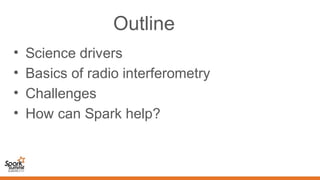
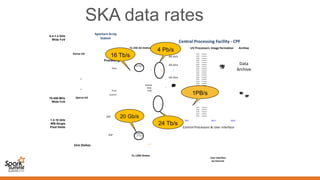
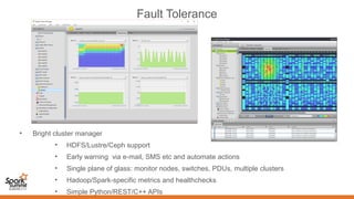
![Five Key Science Areas for the SKA
Topic Goals
Probing the Dark Ages
1. Map out structure formation using HI from the era of
reionization (6 < z < 13)
2. Probe early star formation using high-z CO
3. Detect the first light-emitting sources
Gravity: Pulsars & Black Holes
1. Precision timing of pulsars to test theories of gravity
approaching the strong-field limit (NS-NS,
NS-BH binaries, incl Sgr A*)
2. Millisecond pulsar timing array for detecting long-
wavelength gravitational waves
Cosmic Structure
1. Understand dark energy [e.g. eqn. of state; W(z)]
2. Understand structure formation and galaxy evolution
3. Map and understand dark matter
Cosmic Magnetism
Determine the structure and origins of cosmic magnetic
fields (in galaxies and in the intergalactic medium) vs.
redshift z
The Cradle of Life
1. Understand the formation of Earth-like planets
2. Understand the chemistry of organic molecules and
their roles in planet formation and
generation of life
3. Detect signals from ET
+ serendipitous
discoveries](https://image.slidesharecdn.com/02plabropoulossyatawatta3-151103201534-lva1-app6892/85/Distributed-Data-Processing-using-Spark-by-Panos-Labropoulos_and-Sarod-Yatawatta-17-320.jpg)
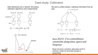


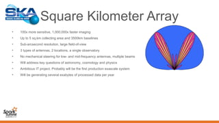
Spark can help with distributed data processing for radio astronomy in three key ways: 1. It allows for in-memory distributed processing of very large datasets across clusters in a fault-tolerant manner, avoiding unnecessary data movement. This is crucial for processing the exabytes of data expected from projects like the Square Kilometer Array. 2. Spark supports iterative algorithms well through its Resilient Distributed Datasets (RDDs) abstraction, which is important for techniques like calibration and deconvolution. 3. Spark can implement consensus-based distributed optimization algorithms to help with calibration, allowing information to be collectively optimized from data distributed across a network.


