Download to read offline
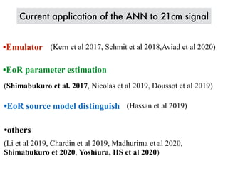
![Red : cosmology Blue : astrophysicsTb =
TS T
1 + z
(1 exp(⌧⌫))
⇠ 27xH(1 + m)
✓
H
dvr/dr + H
◆ ✓
1
T
TS
◆ ✓
1 + z
10
0.15
⌦mh2
◆1/2 ✓
⌦bh2
0.023
◆
[mK]
Brightness temperature
21cm power spectrum (PS) : h Tb(k) Tb(k
0
)i = (2⇡)3
(k + k
0
)P21
Scale dependence
21cm line signal](https://image.slidesharecdn.com/21cmann-201012080249/85/21cm-cosmology-with-ANN-5-320.jpg)
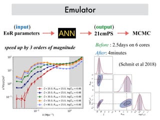
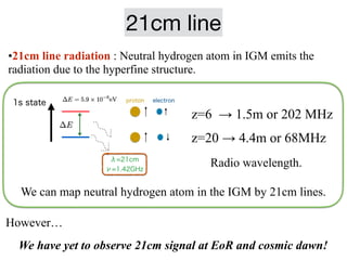
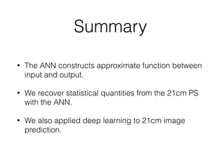
![z=9, 10, 11. PS with thermal noise and cosmic variance
Reconstructed by 21cm PS at z=9,10,11
Rmfp ⇣
Tvir
10
20
30
40
50
60
10 20 30 40 50 60
Rmfp,ANN[Mpc]
Rmfp,true[Mpc]
10
20
30
40
50
60
10 20 30 40 50 60
ζANN
ζtrue
1
10
100
1 10 100
Tvir,ANN[K/10
3
]
Tvir,true[K/10
3
]
Red : z=9,10,11
Blue : z=9
EoR parameters can be reconstructed from
21cm PS well.
Shimabukuro & Semelin, 2017](https://image.slidesharecdn.com/21cmann-201012080249/85/21cm-cosmology-with-ANN-12-320.jpg)

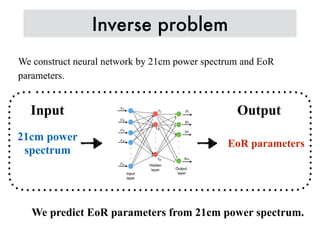
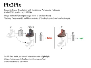
![Power spectrum
21cm power spectrum
.
.
o
n
αesc
˙Nion,int[number/yr], (4)
fesc,c, critical halo mass Mturn =1010
,
.
lanetto 2007 Zahn 2011, 21cmFAST
. R ,
,
)tage (5)
(x) R
, tage z = 15 z = 6.6
,
l(R) (6)
, Vcell . R
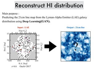
work is trained using ‘H-f02’ model at neutral f
ber 2 and the input is LAE of ‘H-mid’ model at
bin number 3, the output image is named “Hf02
models used in this work is listed in Table. 3.
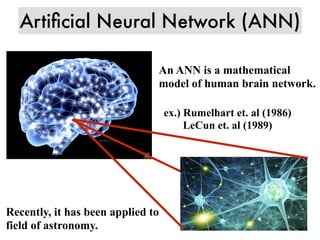
A measure tool to study the 21cm line is the a
trum, which is given by
Pi(|k|) = (2π)2
δD(k − k′
)⟨δi(k)δ∗
i (k′
)⟩
where k is wavenumber in 2D Fourier space an
observation or the output of network. The auto
of observed data (reconstruct image) is repre
Ppix. To detect the 21cm signal from the 21
we consider the cross correlation between the
and reconstruct image, which is given as
PX (|k|) = (2π)2
δD⟨δobs(k)δ∗
pix(k′
)⟩
where δobs and δpix are fluctuation in observe
construct image, respectively. The correlatio
given as
PX (k)
Red : true
Black : output
This result indicates that the network successes to learn statistical property
of the 21cm-line fluctuations.
S. Yoshiura et al.](https://image.slidesharecdn.com/21cmann-201012080249/85/21cm-cosmology-with-ANN-22-320.jpg)


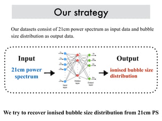
The document discusses using artificial neural networks (ANNs) to analyze 21cm cosmology data. Specifically, it discusses using ANNs to: 1) Emulate and speed up computation of 21cm power spectra from EoR parameters by 3 orders of magnitude. 2) Reconstruct EoR parameters like the mean free path and virial temperature from 21cm power spectra. 3) Recover the ionized bubble size distribution from 21cm power spectra to learn about the EoR source properties. 4) Generate 21cm distributions from Lyman-alpha emitter galaxy distributions using generative adversarial networks.