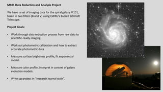
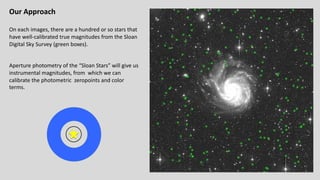
The M101 data reduction and analysis project aims to process imaging data of the spiral galaxy M101 from the Burrell Schmidt telescope using two filters (B and V). The project involves steps like photometric calibration, measuring surface brightness and color profiles, and combining individual images for enhanced quality by correcting for various image contaminants. The final goal is to prepare scientific-ready images and write up the findings in a research journal style.

1. M101 Data Reduction and Analysis Project
We have a set of imaging data for the spiral galaxy M101,
taken in two filters (B and V) using CWRU’s Burrell Schmidt
Telescope.
Project Goals:
• Work through data reduction process from raw data to
scientific-ready imaging.
• Work out photometric calibration and how to extract
accurate photometric data
• Measure surface brightness profile, fit exponential
model.
• Measure color profile, interpret in context of galaxy
evolution models.
• Write up project in “research journal style”.

2. Why so many images?
We can digitally combine
individual images together
into one master image of
much better depth and quality.
Advantage #1: Increase exposure time and signal-to-noise.
Advantage #2: Correct for image contaminants (cosmic rays, satellite trails,
scattered light)
Advantage #3: Correct for detector problems (bad columns, flat fielding
variations, etc)
Advantage #4: Reduce observing risk. (If something goes wrong, you only lose
one exposure!)
Filter Season Number
of Images
Exposure
time
B Spring 2009 8 1200s
V Spring 2010 8 900s
Dithering: the telescope is pointed differently each time so that the
galaxy shows up in a different spot on the detector ⇒

3. Remember the concept of image math and image combining
Images can be thought of as 2D arrays or matrices of intensity values
Images can be added, subtracted, multiplied, and divided by one another, or by a
single value. This is done on a pixel by pixel basis.
An “image stack” can be thought of as a 3D array,
with the third dimension being the different
images in the stack.
When we do an “average” or “median” combine,
we are averaging or medianing the values of each
pixel down the third dimension (ie, the stack).

4. Basic Reduction to Individual images
Remember CCD data reduction steps
• Zero correction
• take many zero-second images without exposing the CCD to light.
• Average them together to create a “master zero” showing fixed pattern noise.
• Subtract that master zero from all the “object frames”
• Flat fielding
• Divide the object images by a “flat field” image: an image showing
sensitivity/gain variations across the image.
• Since the sensitivity is wavelength dependent, each filter must have its own
flat field.

5. Recapping what we did last time
• We examined the zero images, looked at the random read noise level (~ 1.5
ADU/pix), verified it was consistant.
• We averaged 16 zero images together to make a ”master zero”. In that master zero
we saw the noise level went down and we could see the residual “fixed pattern
noise”
• We examined the flat field, saw the variations due to in sensitivity and gain issues.
• We took the object images, subtracted off the master zero, then divided by the
flat field to produce reduced images.
Next steps: Photometric calibration and Sky subtraction

6. Photometric Calibration
Images were taken at different airmasses (and sometimes on different nights) so they have different photometric
properties. The same star will produce fewer counts when observed at greater airmass. We can’t just average all the
images together, we have to scale them in intensity to a “common zeropoint” to correct for the photometric differences.
Method #1: Observe standard stars, work out overall photometric solution, then apply to object images:
𝑚!"#$ − 𝑚% = 𝐶% 𝐵 − 𝑉 + 𝐾% sec(𝑧) + 𝑍𝑃%
Why the color term? Our filters are slightly different from standard
Johnson B and V filters.
The brightness of the star will be a bit different through our filters than
through standard B, V filters, and the difference will depend on the
color of the star.
wavelength
transmission
remember: instrumental magnitude is
just a logarithmic measure of
uncalibrated flux on the detector:
𝑚!"#$ = −2.5 log(𝐴𝐷𝑈/𝑡𝑖𝑚𝑒) + 𝑐𝑜𝑛𝑠𝑡

7. Photometric Calibration
Images were taken at different airmasses (and sometimes on different nights) so they have different photometric
properties. The same star will produce fewer counts when observed at greater airmass. We can’t just average all the
images together, we have to scale them in intensity to a “common zeropoint” to correct for the photometric differences.
Method #2 (What we will do): If you have many stars of known brightness (𝑚%) and 𝐵 − 𝑉 color on your object
images, you can calibrate the solution directly for each image:
𝑚!"#$ − 𝑚% = 𝐶% 𝐵 − 𝑉 + 𝑍𝑃%,'()*+
where 𝑍𝑃%,'()*+ = 𝐾% sec(𝑧) + 𝑍𝑃%.
Each star on a given image gives a value for 𝑚!"#$ − 𝑚% and 𝐵 − 𝑉 , so plot 𝑚!"#$ − 𝑚% against 𝐵 − 𝑉 for many
stars on the image, and then fit a line:
• 𝐶% = slope
• 𝑍𝑃%,'()*+ = intercept

8. Our Approach
On each images, there are a hundred or so stars that
have well-calibrated true magnitudes from the Sloan
Digital Sky Survey (green boxes).
Aperture photometry of the “Sloan Stars” will give us
instrumental magnitudes, from which we can
calibrate the photometric zeropoints and color
terms.

9. For each image, we calculate an instrumental
magnitude for SDSS stars on the field:
𝑚!"#$ = −2.5 log ⁄
𝐼),- 𝑡./0 + 25
then calibrate a photometric solution
𝑚!"#$ − 𝑚% = 𝐶% 𝐵 − 𝑉 + 𝑍𝑃%,'()*+
Note how errors build up at every step
• The S/N calculation tell you the errors in
measuring the flux.
• The errors in the photometric solution add
to that uncertainty when calculating a
calibrated magnitude. 𝐶% (slope) = 0.262 ± 0.027
𝑍𝑃%,'()*+ intercept = 3.670 ± 0.017
obj0419029.fits

10. Sky Subtraction
Sky brightness can change from night to night, and over the course of a single night, and also depends on airmass and
direction you are observing. So the images all have different sky levels and we have to subtract off this sky level before
combining.
Method #1: Measure sky at many spots across the image, work out an average value, subtract that value off the image.
SKY = average sky

11. But the sky level may not
be uniform across the
image!
So a constant sky value
may not be a great model.

12. Sky Subtraction
Sky brightness can change from night to night, and over the course of a single night, and also depends on airmass and
direction you are observing. So the images all have different sky levels and we have to subtract off this sky level before
combining.
Method #2 (what we will do): Measure sky at many spots across the image, fit a plane to the sky level as a function of
X,Y position on the image.
𝑆𝐾𝑌 = 𝑋×∇123,4 + 𝑌×∇123,3+𝑆𝐾𝑌5
where ∇123,4 and ∇123,3 are the sky gradients in the X and Y direction on the image, respectively, 𝑆𝐾𝑌5 is an average
sky level.
How do we do this? Use the sky estimate around each
Sloan star (from the photometric calibration step) as a
function of X and Y to fit and subtract a sky plane
from each image.

13. Astronomical Image File Formats: FITS images
Images are in FITS format, consisting of two parts:
Image: array of pixel intensity values Header: information about the image
KEYWORD = ‘VALUE’ / comment
Tip: In ds9, view the
header via File --> Header

14. Photometric Solution fit for the B-band image obj0419029.fits:
𝑚!"#$ − 𝑚% = 𝐶% 𝐵 − 𝑉 + 𝑍𝑃%,'()*+
𝐶% (slope) = 0.262 ± 0.027
𝑍𝑃%,'()*+ intercept = 3.670 ± 0.017
Fit a line to the data to estimate color term and zeropoint.
Remember instrumental magnitude:
𝑚!"#$ = −2.5 log ⁄
𝐼%&' 𝑡()* + 25

15. Sky values as a function of X and Y for the B-band image obj0419029.fits:
𝑆𝐾𝑌 = 𝑋×∇123,4 + 𝑌×∇123,3 + 𝑆𝐾𝑌5
∇123,4= 1.468 ±0.082 × 1067
ADU/pix
∇123,3= 0.440 ±0.084 × 1067
ADU/pix
𝑆𝐾𝑌5 = 606.50 ± 0.27 ADU
Fit and subtract a 2D plane to remove the sky background.

16. This process (calibration and sky subtraction) prepares each image for combining. We do this for all images in the B
and V image sets,
CalibrateImages.ipyb calculates photometric solutions for all images and write out new versions of each image with
the sky levels subtracted off.
Look at photometric solutions and sky
levels for the B-band images.
Differences in color term
Mostly random scatter
Differences in zeropoint
Real, systematic changes. Images
were taken at different airmasses
Differences is sky level
Real, systematic changes. Images
were taken at different airmasses and
times.

17. What’s next?
Each image also has contamination/noise in it due to:
• CCD Read noise (remember: subtracting off the master eliminates the fixed pattern noise, but not the
random read noise. That cannot be removed from an individual image.
• Variations in sky intensity
• Scattered light and reflections inside the telescope
• Satellites passing through the field of view
• Bad pixels and columns in the CCD
• Cosmic rays
To reduce noise and remove contamination, we want to
• shift each image so that M101 is at the same spot
• scale each image to a common intensity
• do a median stack of all the images.

18. Shifting the images to a common center: “Image re-registration”
Simplest version: XY integer pixel shift (“shift flux in each pixel over 100 pixels and down 200 pixels”)
In reality: non-integer XY shifts, plus rotation. Geometric transformation is mathematically intensive, and introduces
additional uncertainty into the data.
Original Image Re-registered Image

19. Applying Zeropoints: Photometric Scaling
The same star will have different numbers of counts in each image due to the different zeropoints. We can
define a “final zeropoint” and scale each image up or down in intensity to match this average zeropoint.
ZP_FINAL = np.average(ZP_image)
Since zeropoints are in magnitudes, we can say
𝑍𝑃8!"9: − 𝑍𝑃!;9<. = −2.5 log ⁄
𝐼8!"9: 𝐼!;9<.
Then we scale each image in intensity by a factor of
𝐼8!"9: = 𝐼!;9<.× 1065.> ?@!"#$%6?@"&$'(
That 10^ term is the photometric scaling we multiply each image by to get them on the same final zeropoint. After
scaling all the images this way, a given star should have the same number of counts (+/- noise) in each image.

20. Final Image Combine
1. Scale each image in intensity to match the average zeropoint:
𝐼#A9:.B = 𝐼!;9<.× 1065.> ?@$)'6?@"&$'(
2. Re-register each image so that M101 is at the center of the image.
3. Create a final image by calculating a the median pixel intensity along a stack of the shifted, scaled
images.
This takes 3-5 minutes…..

21. Applying your photometric solution to the final combined images
Part 1: Instrumental magnitudes
In the notebooks, we defined Instrumental magnitudes in terms of counts/second:
𝑚!"#$ = −2.5 log ⁄
𝐼 𝑡./0 + 25
So in analyzing the reduced images, we need to define our instrumental magnitudes the
same way.
And since we medianed the images (rather than summing them), 𝑡./0 is the exposure time
of an individual image:
• V images: 900 seconds (15 mins)
• B images: 1200 seconds (20 mins)
So turn counts into instrumental magnitudes using those values.

22. Applying your photometric solution to the final combined images
Part 2: Turn instrumental magnitudes into real magnitudes
Our photometric solution:
𝑚!"#$,% − 𝑚% = 𝐶% 𝐵 − 𝑉 + 𝑍𝑃%
𝑚!"#$,C − 𝑚C = 𝐶C 𝐵 − 𝑉 + 𝑍𝑃C
FINAL B V
C 0.277 0.233
ZP 3.619 3.541
EXPTIME 1200 900

23. Applying your photometric solution to the final combined images
Part 2: Turn instrumental magnitudes into real magnitudes
Our photometric solution:
𝑚% = 𝑚!"#$,% − 𝐶% 𝐵 − 𝑉 − 𝑍𝑃%
𝑚C = 𝑚!"#$,C − 𝐶C 𝐵 − 𝑉 − 𝑍𝑃C
FINAL B V
C 0.277 0.233
ZP 3.619 3.541
EXPTIME 1200 900

24. Applying your photometric solution to the final combined images
Part 2: Turn instrumental magnitudes into real magnitudes
Our photometric solution:
𝑚% = 𝑚!"#$,% − 𝐶% 𝐵 − 𝑉 − 𝑍𝑃%
𝑚C = 𝑚!"#$,C − 𝐶C 𝐵 − 𝑉 − 𝑍𝑃C
But wait…
Subtract one from the other:
𝑚% − 𝑚C = 𝑚!"#$,% − 𝑚!"#$,C − 𝐶% − 𝐶C 𝐵 − 𝑉 − 𝑍𝑃% − 𝑍𝑃C
𝐵 − 𝑉 = 𝑚!"#$,% − 𝑚!"#$,C − 𝐶% − 𝐶C 𝐵 − 𝑉 − 𝑍𝑃% − 𝑍𝑃C
𝐵 − 𝑉 1 + 𝐶% − 𝐶C = 𝑚!"#$,% − 𝑚!"#$,C − 𝑍𝑃% − 𝑍𝑃C
𝐵 − 𝑉 = Q
𝑚!"#$,% − 𝑚!"#$,C − 𝑍𝑃% − 𝑍𝑃C 1 + 𝐶% − 𝐶C
FINAL B V
C 0.277 0.233
ZP 3.619 3.541
EXPTIME 1200 900

25. Applying your photometric solution to the final combined images
Summary
First measure counts and calculate instrumental magnitudes in each filter:
𝑚!"#$,% = −2.5 log ⁄
𝐼% 𝑡./0,% + 25
𝑚!"#$,C = −2.5 log ⁄
𝐼C 𝑡./0,C + 25
Then calculate the color:
𝐵 − 𝑉 = Q
𝑚!"#$,% − 𝑚!"#$,C − 𝑍𝑃% − 𝑍𝑃C 1 + 𝐶% − 𝐶C
Then insert that color into the photometric solution to calculate magnitudes:
𝑚% = 𝑚!"#$,% − 𝐶% 𝐵 − 𝑉 − 𝑍𝑃%
𝑚C = 𝑚!"#$,C − 𝐶C 𝐵 − 𝑉 − 𝑍𝑃C
FINAL B V
C 0.277 0.233
ZP 3.619 3.541
EXPTIME 1200 900

26. One last step – correcting for galactic extinction
After all photometry is done and you have your “final” magnitudes and colors, you want to
correct for galactic extinction. Dust in the Milky Way (which we are looking through) both
dims and reddens the light from M101.
Look up the galactic extinction on NED, using the estimate from Schlafly and Finkbeiner
(2011). Then correct for extinction in each band by doing:
𝑚%,5 = 𝑚%,DE# − 𝐴%
𝑚C,5 = 𝑚C,DE# − 𝐴C
And then correct the color by doing either
𝐵 − 𝑉 5 = 𝐵 − 𝑉 DE# − (𝐴% − 𝐴C)
or
𝐵 − 𝑉 5 = 𝑚%,5 − 𝑚C,5
But not both! That is, don’t calculate your color from the corrected magnitude and then
also apply the reddening correction.

27. Applying your photometric solution to the final combined images
Summary
First measure counts and calculate instrumental magnitudes in each filter:
𝑚!"#$,% = −2.5 log ⁄
𝐼% 𝑡./0,% + 25
𝑚!"#$,C = −2.5 log ⁄
𝐼C 𝑡./0,C + 25
Then calculate the color:
𝐵 − 𝑉 = Q
𝑚!"#$,% − 𝑚!"#$,C − 𝑍𝑃% − 𝑍𝑃C 1 + 𝐶% − 𝐶C
Then insert that color into the photometric solution to calculate magnitudes:
𝑚% = 𝑚!"#$,% − 𝐶% 𝐵 − 𝑉 − 𝑍𝑃%
𝑚C = 𝑚!"#$,C − 𝐶C 𝐵 − 𝑉 − 𝑍𝑃C
FINAL B V
C
ZP
EXPTIME 1200 900
Fill in this table using the info
from the image headers ⇒

28. Working with your final combined images
In a terminal window:
• cd ~/M101
• mv Bdata/stack_med.fits M101B.fits
• mv Vdata/stack_med.fits M101V.fits
• ds9 M101B.fits M101V.fits &
In ds9:
• Frame à Single Frame
• Frame à Lock à Frame à WCS
• Scale à Scale Parameters à -10 to 3,000
• Scale à Log
• Frame à Lock à Scale
• Frame à Lock à Colorbar
ds9 regions (Regions à Shape):
• Ruler: will measure distances on image in different units
• Circles: for photometry
• Make region around object, measure total flux in object
• Move region to nearby blank sky, measure total flux in blank sky
• Subtract blank sky flux from object flux to get total flux
• You can also enter a 𝛼, 𝛿 or 𝑋, 𝑌 coordinate for the region center and it
will move to that position.
This sets up ds9 so you can zoom,
pan, and change the display
stretch on one image, then hit
“tab” and see the other image
similarly displayed.