STA6166-RegBasics 1
Regression Basics(§11.1 – 11.3)
Regression Unit Outline
• What is Regression?
• How is a Simple Linear Regression Analysis done?
• Outline the analysis protocol.
• Work an example.
• Examine the details (a little theory).
• Related items.
• When is simple linear regression appropriate?
2.
STA6166-RegBasics 2
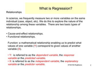
Relationships
In science,we frequently measure two or more variables on the same
individual (case, object, etc). We do this to explore the nature of the
relationship among these variables. There are two basic types of
relationships.
• Cause-and-effect relationships.
• Functional relationships.
Function: a mathematical relationship enabling us to predict what
values of one variable (Y) correspond to given values of another
variable (X).
• Y: is referred to as the dependent variable, the response
variable or the predicted variable.
• X: is referred to as the independent variable, the explanatory
variable or the predictor variable.
What is Regression?
3.
STA6166-RegBasics 3
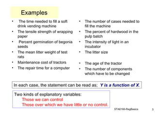
Examples
• Thetime needed to fill a soft
drink vending machine
• The tensile strength of wrapping
paper
• Percent germination of begonia
seeds
• The mean litter weight of test
rats
• Maintenance cost of tractors
• The repair time for a computer
• The number of cases needed to
fill the machine
• The percent of hardwood in the
pulp batch
• The intensity of light in an
incubator
• The litter size
• The age of the tractor
• The number of components
which have to be changed
In each case, the statement can be read as; Y is a function of X.
Two kinds of explanatory variables:
Those we can control
Those over which we have little or no control.
4.
STA6166-RegBasics 4
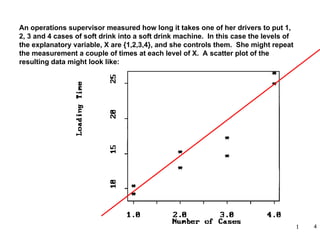
An operationssupervisor measured how long it takes one of her drivers to put 1,
2, 3 and 4 cases of soft drink into a soft drink machine. In this case the levels of
the explanatory variable, X are {1,2,3,4}, and she controls them. She might repeat
the measurement a couple of times at each level of X. A scatter plot of the
resulting data might look like:
5.
STA6166-RegBasics 5
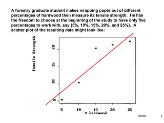
A forestrygraduate student makes wrapping paper out of different
percentages of hardwood then measure its tensile strength. He has
the freedom to choose at the beginning of the study to have only five
percentages to work with, say {5%, 10%, 15%, 20%, and 25%}. A
scatter plot of the resulting data might look like:
6.
STA6166-RegBasics 6
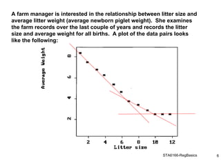
A farmmanager is interested in the relationship between litter size and
average litter weight (average newborn piglet weight). She examines
the farm records over the last couple of years and records the litter
size and average weight for all births. A plot of the data pairs looks
like the following:
7.
STA6166-RegBasics 7
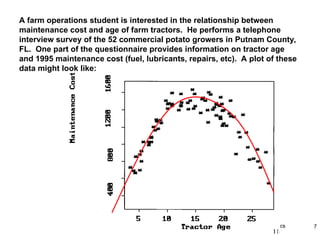
A farmoperations student is interested in the relationship between
maintenance cost and age of farm tractors. He performs a telephone
interview survey of the 52 commercial potato growers in Putnam County,
FL. One part of the questionnaire provides information on tractor age
and 1995 maintenance cost (fuel, lubricants, repairs, etc). A plot of these
data might look like:
8.
STA6166-RegBasics 8
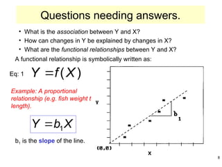
• Whatis the association between Y and X?
• How can changes in Y be explained by changes in X?
• What are the functional relationships between Y and X?
A functional relationship is symbolically written as:
)
(X
f
Y
Eq: 1
Example: A proportional
relationship (e.g. fish weight to
length).
X
b
Y 1
b1 is the slope of the line.
Questions needing answers.
9.
STA6166-RegBasics 9
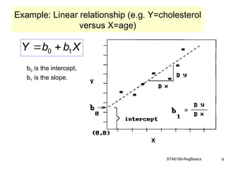
b0 isthe intercept,
b1 is the slope.
X
b
b
Y 1
0
Example: Linear relationship (e.g. Y=cholesterol
versus X=age)
10.
STA6166-RegBasics 10
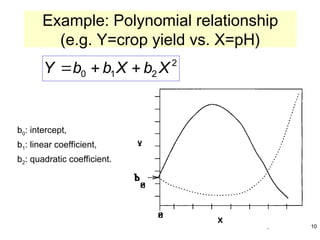
b0: intercept,
b1:linear coefficient,
b2: quadratic coefficient.
2
2
1
0 X
b
X
b
b
Y
Example: Polynomial relationship
(e.g. Y=crop yield vs. X=pH)
STA6166-RegBasics 12
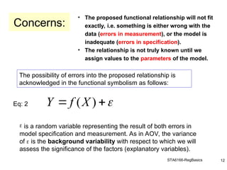
• Theproposed functional relationship will not fit
exactly, i.e. something is either wrong with the
data (errors in measurement), or the model is
inadequate (errors in specification).
• The relationship is not truly known until we
assign values to the parameters of the model.
The possibility of errors into the proposed relationship is
acknowledged in the functional symbolism as follows:
)
(X
f
Y
Eq: 2
is a random variable representing the result of both errors in
model specification and measurement. As in AOV, the variance
of is the background variability with respect to which we will
assess the significance of the factors (explanatory variables).
Concerns:
13.
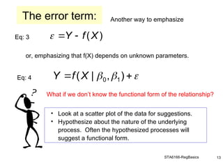
STA6166-RegBasics 13
Another wayto emphasize
)
(X
f
Y
Eq: 3
or, emphasizing that f(X) depends on unknown parameters.
)
,
|
( 1
0
X
f
Y
Eq: 4
What if we don’t know the functional form of the relationship?
• Look at a scatter plot of the data for suggestions.
• Hypothesize about the nature of the underlying
process. Often the hypothesized processes will
suggest a functional form.
The error term:
14.
STA6166-RegBasics 14
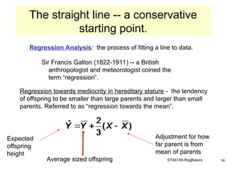
Regression Analysis:the process of fitting a line to data.
Sir Francis Galton (1822-1911) -- a British
anthropologist and meteorologist coined the
term “regression”.
Regression towards mediocrity in hereditary stature - the tendency
of offspring to be smaller than large parents and larger than small
parents. Referred to as “regression towards the mean”.
)
(
3
2
ˆ X
X
Y
Y
The straight line -- a conservative
starting point.
)
(
3
2
ˆ X
X
Y
Y
Average sized offspring
Adjustment for how
far parent is from
mean of parents
Expected
offspring
height
15.
STA6166-RegBasics 15
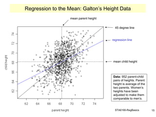
Regression tothe Mean: Galton’s Height Data
45 degree line
regression line
mean child height
mean parent height
mean parent height
Data: 952 parent-child
pairs of heights. Parent
height is average of the
two parents. Women’s
heights have been
adjusted to make them
comparable to men’s.
16.
STA6166-RegBasics 16
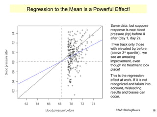
Regression tothe Mean is a Powerful Effect!
Same data, but suppose
response is now blood
pressure (bp) before &
after (day 1, day 2).
If we track only those
with elevated bp before
(above 3rd
quartile) , we
see an amazing
improvement, even
though no treatment took
place!
This is the regression
effect at work. If it is not
recognized and taken into
account, misleading
results and biases can
occur.
STA6166-RegBasics 18
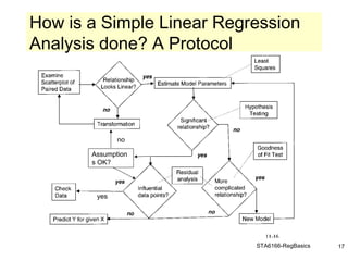
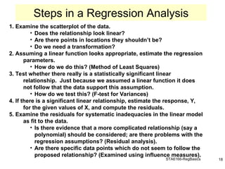
1. Examinethe scatterplot of the data.
• Does the relationship look linear?
• Are there points in locations they shouldn’t be?
• Do we need a transformation?
2. Assuming a linear function looks appropriate, estimate the regression
parameters.
• How do we do this? (Method of Least Squares)
3. Test whether there really is a statistically significant linear
relationship. Just because we assumed a linear function it does
not follow that the data support this assumption.
• How do we test this? (F-test for Variances)
4. If there is a significant linear relationship, estimate the response, Y,
for the given values of X, and compute the residuals.
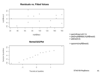
5. Examine the residuals for systematic inadequacies in the linear model
as fit to the data.
• Is there evidence that a more complicated relationship (say a
polynomial) should be considered; are there problems with the
regression assumptions? (Residual analysis).
• Are there specific data points which do not seem to follow the
proposed relationship? (Examined using influence measures).
Steps in a Regression Analysis
19.
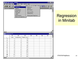
STA6166-RegBasics 19
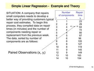
SITUATION: Acompany that repairs
small computers needs to develop a
better way of providing customers typical
repair cost estimates. To begin this
process, they compiled data on repair
times (in minutes) and the number of
components needing repair or
replacement from the previous week.
The data, sorted by number of
components are as follows:
Number Repair
of components time
i xi yi
1 1 23
2 2 29
3 4 64
4 4 72
5 4 80
6 5 87
7 6 96
8 6 105
9 8 127
10 8 119
11 9 145
12 9 149
13 10 165
14 10 154
Paired Observations (xi, yi)
Simple Linear Regression - Example and Theory
20.
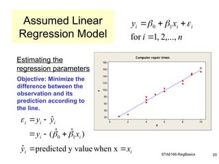
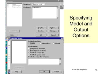
STA6166-RegBasics 20
Estimating the
regressionparameters
Objective: Minimize the
difference between the
observation and its
prediction according to
the line.
Assumed Linear
Regression Model n
i
x
y i
i
i
,...,
2
,
1
for
1
0
)
ˆ
ˆ
(
ˆ
1
0 i
i
i
i
i
x
y
y
y
X
Y
10
8
6
4
2
0
180
160
140
120
100
80
60
40
20
Computer repair times
i
i x
y
when x
y value
predicted
ˆ
21.
STA6166-RegBasics 21
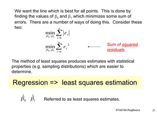
We wantthe line which is best for all points. This is done by
finding the values of 0 and 1 which minimizes some sum of
errors. There are a number of ways of doing this. Consider these
two:
The method of least squares produces estimates with statistical
properties (e.g. sampling distributions) which are easier to
determine.
Referred to as least squares estimates.
Sum of squared
residuals
Regression => least squares estimation
n
i
i
n
i
i
1
2
,
1
,
1
0
1
0
min
min
1
0
ˆ
ˆ
22.
STA6166-RegBasics 22
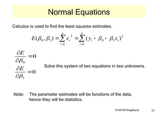
Calculus isused to find the least squares estimates.
Solve this system of two equations in two unknowns.
Note: The parameter estimates will be functions of the data,
hence they will be statistics.
Normal Equations
n
i
i
i
n
i
i x
y
E
1
2
1
0
1
2
1
0 )
(
)
,
(
0
0
1
0
E
E
23.
STA6166-RegBasics 23
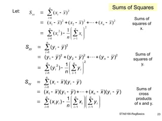
Let:
n
i
n
i
i
i
n
n
i
i
xx
x
n
x
x
x
x
x
x
x
x
x
S
1
2
1
2
2
2
2
2
1
1
2
1
)
(
)
(
)
(
)
(
)
(
n
i
n
i
i
i
n
n
i
i
yy
y
n
y
y
y
y
y
y
y
y
y
S
1
2
1
2
2
2
2
2
1
1
2
1
)
(
)
(
)
(
)
(
)
(
n
i
n
i
i
n
i
i
i
i
i
n
n
i
i
i
xy
y
x
n
y
x
y
y
x
x
y
y
x
x
y
y
x
x
S
1 1
1
1
1
1
1
)
(
)
)(
(
)
)(
(
)
)(
(
Sums of
squares of
x.
Sums of
squares of
y.
Sums of
cross
products
of x and y.
Sums of Squares
24.
STA6166-RegBasics 24
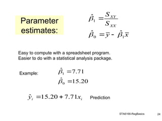
Easy tocompute with a spreadsheet program.
Easier to do with a statistical analysis package.
Example:
Prediction
Parameter
estimates: x
y
S
S
XX
XY
1
0
1
ˆ
ˆ
ˆ
20
.
15
ˆ
71
.
7
ˆ
0
1
i
i x
y 71
.
7
20
.
15
ˆ
25.
STA6166-RegBasics 25
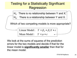
Ho: Thereis no relationship between Y and X.
HA: There is a relationship between Y and X.
Which of two competing models is more appropriate?
We look at the sums of squares of the prediction
errors for the two models and decide if that for the
linear model is significantly smaller than that for
the mean model.
Testing for a Statistically Significant
Regression
Y
X
Y
:
Model
Mean
:
Model
Linear 1
0
26.
STA6166-RegBasics 26
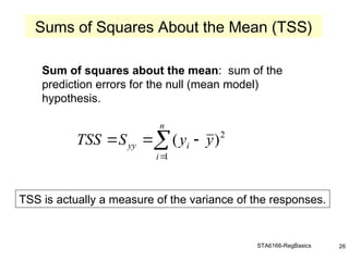
Sum ofsquares about the mean: sum of the
prediction errors for the null (mean model)
hypothesis.
Sums of Squares About the Mean (TSS)
TSS is actually a measure of the variance of the responses.
n
i
i
yy y
y
S
TSS
1
2
)
(
27.
STA6166-RegBasics 27
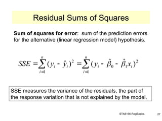
Residual Sumsof Squares
Sum of squares for error: sum of the prediction errors
for the alternative (linear regression model) hypothesis.
SSE measures the variance of the residuals, the part of
the response variation that is not explained by the model.
n
i
i
i
n
i
i
i x
y
y
y
SSE
1
2
1
0
1
2
)
ˆ
ˆ
(
)
ˆ
(
28.
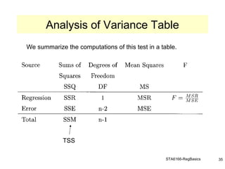
STA6166-RegBasics 28
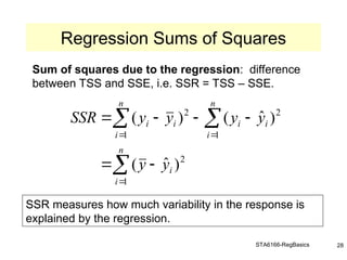
Regression Sumsof Squares
Sum of squares due to the regression: difference
between TSS and SSE, i.e. SSR = TSS – SSE.
SSR measures how much variability in the response is
explained by the regression.
n
i
i
n
i
i
i
n
i
i
i
y
y
y
y
y
y
SSR
1
2
1
2
1
2
)
ˆ
(
)
ˆ
(
)
(
29.
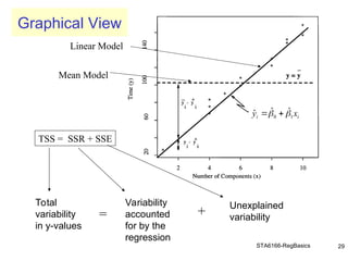
STA6166-RegBasics 29
i
i x
y1
0
ˆ
ˆ
ˆ
Mean Model
Linear Model
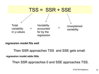
Total
variability
in y-values
=
Variability
accounted
for by the
regression
+
Unexplained
variability
TSS = SSR + SSE
Graphical View
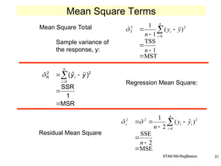
STA6166-RegBasics 31
Sample varianceof
the response, y:
MST
1
TSS
)
(
1
1
ˆ
1
2
2
T
n
y
y
n
n
i
i
Mean Square Total
Regression Mean Square:
MSR
1
SSR
)
ˆ
(
ˆ
1
2
2
R
n
i
i y
y
MSE
2
SSE
)
ˆ
(
2
1
ˆ
ˆ
1
2
2
2
n
y
y
n
n
i
i
i
Residual Mean Square
Mean Square Terms
32.
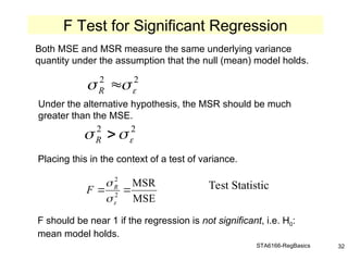
STA6166-RegBasics 32
Both MSEand MSR measure the same underlying variance
quantity under the assumption that the null (mean) model holds.
Under the alternative hypothesis, the MSR should be much
greater than the MSE.
Placing this in the context of a test of variance.
2
2
R
2
2
R
MSE
MSR
2
2
R
F Test Statistic
F should be near 1 if the regression is not significant, i.e. H0:
mean model holds.
F Test for Significant Regression
33.
STA6166-RegBasics 33
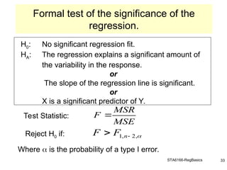
H0: Nosignificant regression fit.
HA: The regression explains a significant amount of
the variability in the response.
or
The slope of the regression line is significant.
or
X is a significant predictor of Y.
Reject H0 if:
Where is the probability of a type I error.
Formal test of the significance of the
regression.
Test Statistic:
,
2
,
1
n
F
F
MSE
MSR
F
34.
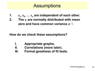
STA6166-RegBasics 34
1. 1,2, … n are independent of each other.
2. The i are normally distributed with mean
zero and have common variance
.
How do we check these assumptions?
I. Appropriate graphs.
II. Correlations (more later).
III. Formal goodness of fit tests.
Assumptions
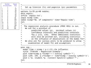
STA6166-RegBasics 36
Number Repair
ofcomponents time
i xi yi
1 1 23
2 2 29
3 4 64
4 4 72
5 4 80
6 5 87
7 6 96
8 6 105
9 8 127
10 8 119
11 9 145
12 9 149
13 10 165
14 10 154
*----------------------------------------------------------*;
* Set up linesize (ls) and pagesize (ps) parameters *;
*----------------------------------------------------------*;
options ls=78 ps=40 nodate;
data repair;
infile 'repair.txt';
input ncomp time;
label ncomp="No. of components" time="Repair time";
run;
*----------------------------------------------------------*;
* The regression analysis procedure (PROC REG) is run. *;
* We ask for a printout of *;
* predicted values (p), residual values (r) *;
* confidence intervals and prediction intervals *;
* for y (cli, clm). Other additional statistics *;
* will also be printed out, including statistics *;
* on the influence of observations on the model fit*;
* We also ask for various plots to be produced to allow *;
* examination of model fit and assumptions *;
*----------------------------------------------------------*;
proc reg ;
model time = ncomp / p r cli clm influence;
title 'STA6166 - Regression Example';
plot time*ncomp p.*ncomp='+'/ overlay symbol='*';
plot (u95. l95. p.)*ncomp='+' time*ncomp / overlay symbol='o';
plot r.*p. student.*p. /collect hplots=2 symbol='*';
run;
*----------------------------------------------------------*;
STA6166-RegBasics 38
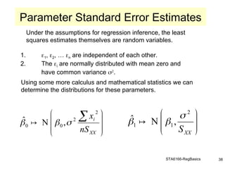
Under theassumptions for regression inference, the least
squares estimates themselves are random variables.
1. 1, 2, … n are independent of each other.
2. The i are normally distributed with mean zero and
have common variance
.
Using some more calculus and mathematical statistics we can
determine the distributions for these parameters.
Parameter Standard Error Estimates
XX
i
nS
x
2
2
0
0 ,
N
ˆ
XX
S
2
1
1 ,
N
ˆ
39.
STA6166-RegBasics 39
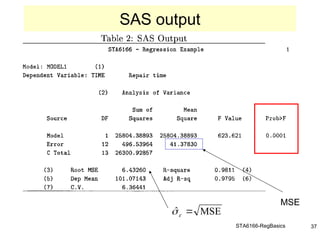
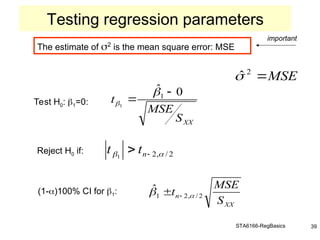
The estimateof 2
is the mean square error: MSE
important
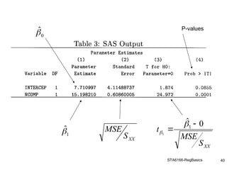
Test H0: 1=0:
Reject H0 if:
(1-)100% CI for 1:
Testing regression parameters
2
/
,
2
1
n
t
t
XX
n
S
MSE
t 2
/
,
2
1
ˆ
MSE
2
ˆ
XX
S
MSE
t
0
ˆ
1
1