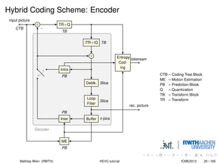
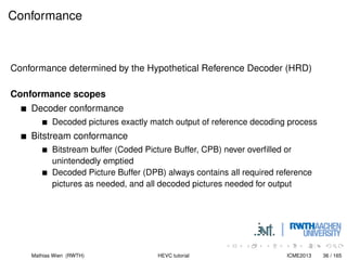
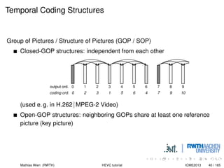
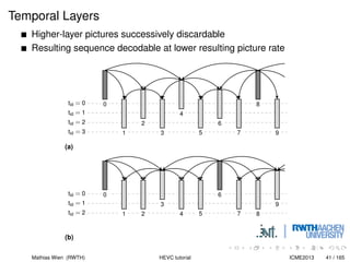
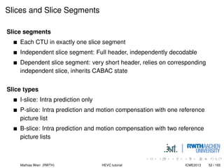
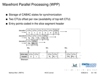
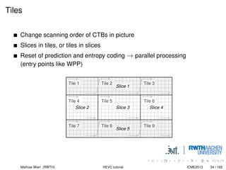
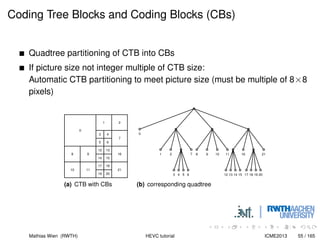
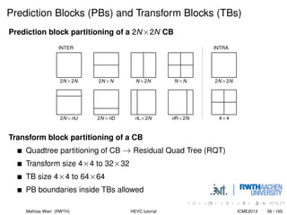
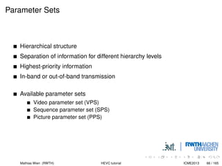
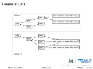
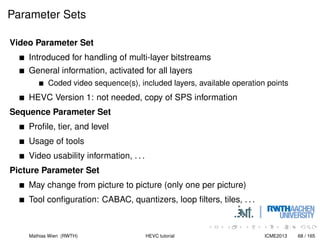
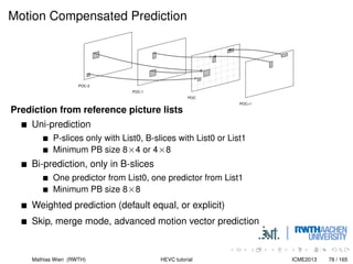
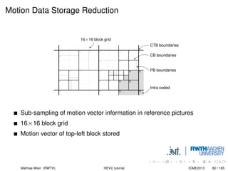
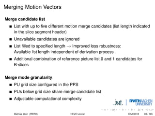
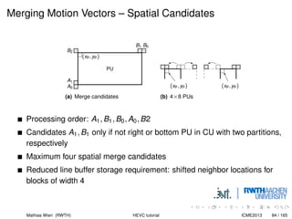
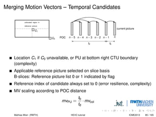
This document provides an outline for a tutorial on High Efficiency Video Coding (HEVC). It discusses the motivation for developing a new video coding standard to support higher resolutions and bandwidth efficiency. It describes the formation of the Joint Collaborative Team on Video Coding (JCT-VC) by MPEG and VCEG to develop the HEVC specification. It also gives an overview of the hybrid coding scheme used in HEVC and other video coding standards, including prediction, transform coding of residuals, and entropy coding.
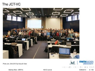
![Joint Collaborative Team on Video Coding – JCT-VC
Previous collaborations between MPEG and ITU-T
H.262|MPEG-2 Video
H.264|AVC in the Joint Video Team (last meeting Nov. 2009 in Geneva)
New collaboration between MPEG and VCEG
Joint Collaborative Team on Video Coding (JCT-VC)
Agreement on Terms of Reference Jan. 2010, N11112, VCEG-AM90 [5]
Joint Call for Proposals issues Jan. 2010, N11113, VCEG-AM91 [6]
1st meeting in Dresden, April 2010
Chairs
Gary J. Sullivan (Microsoft)
Jens-Rainer Ohm (RWTH Aachen University)
Resources
Mathias Wien (RWTH) HEVC tutorial ICME2013 14 / 165](https://image.slidesharecdn.com/tutorialhighefficiencyvideocodingcoding-toolsandspecification-221218095016-665f1135/85/Tutorial-High-Efficiency-Video-Coding-Coding-Tools-and-Specification-pdf-14-320.jpg)
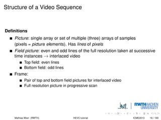
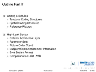
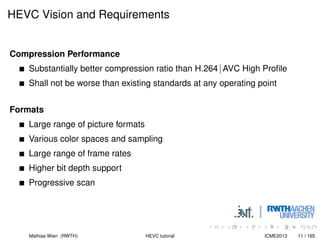
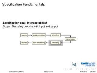
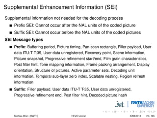
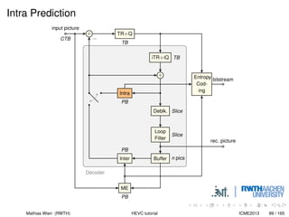
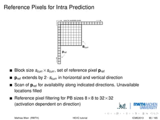
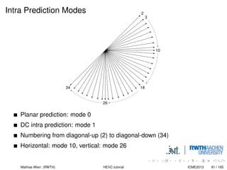
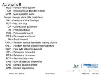
![Representation of Color
Color representation: YCbCr
Luminance (Y): gray-level picture, weighted sum of the RGB components
Chrominance (Cb, Cr): delta of Luminance to single color components
Normalization according to transfer characteristics of capture/display
Luma and chroma components (Y, Cb, Cr)
Sub-sampling of chroma
luma
chroma
(a) YCbCr 4:2:0 (b) YCbCr 4:2:2
further reading: [7]
Mathias Wien (RWTH) HEVC tutorial ICME2013 18 / 165](https://image.slidesharecdn.com/tutorialhighefficiencyvideocodingcoding-toolsandspecification-221218095016-665f1135/85/Tutorial-High-Efficiency-Video-Coding-Coding-Tools-and-Specification-pdf-18-320.jpg)
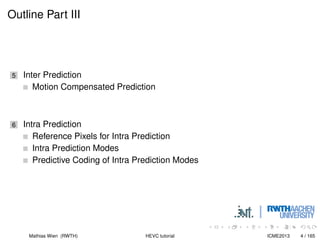
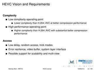
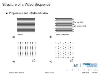
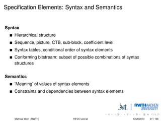
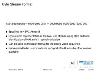
![Bjøntegaard Delta Measurement
0 250 500 750 1000125015001750
35
36
37
38
39
40
41
42
43
44
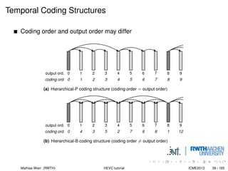
Rate [kbps]
PSNR
Y
[dB]
0 250 500 750 1000125015001750
35
36
37
38
39
40
41
42
43
44
Rate [kbps]
PSNR
Y
[dB]
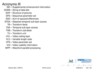
(a) BD-PSNR (b) BD-rate
Comparison of two rate-distortion curves with four rate points
Interpolation of curves (using log-rate)
Polynomial VCEG-M33 [9], or pice-wise cubic JCTVC-F270 [10]
Rate delta (BD-rate, %) or PSNR delta (BD-PSNR, dB) by integration
over intermediate area
Mathias Wien (RWTH) HEVC tutorial ICME2013 24 / 165](https://image.slidesharecdn.com/tutorialhighefficiencyvideocodingcoding-toolsandspecification-221218095016-665f1135/85/Tutorial-High-Efficiency-Video-Coding-Coding-Tools-and-Specification-pdf-24-320.jpg)
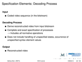
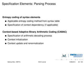
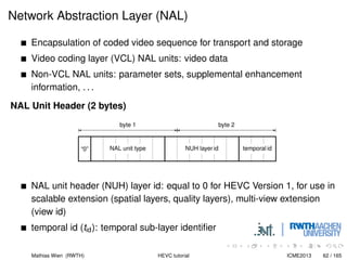
![Specification Principles: Independent Parsing
Parsing independent from decoding
Parsing must be possible in the case of transmission losses
No dependency of occurrence of syntax elements based on properties of
decoded pictures
Independent slice parsing
Slices of a picture must be independent
→ separately decodable in case of slice losses
Enables parallel processing of slices
Further: no parsing dependencies in parameter sets
(e. g. on certain profile) → extensibility
SzBu12 [11]
Mathias Wien (RWTH) HEVC tutorial ICME2013 31 / 165](https://image.slidesharecdn.com/tutorialhighefficiencyvideocodingcoding-toolsandspecification-221218095016-665f1135/85/Tutorial-High-Efficiency-Video-Coding-Coding-Tools-and-Specification-pdf-31-320.jpg)

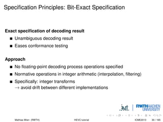
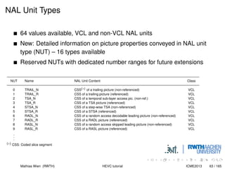
![Specification Principles: Dynamic Range
Memory consumption
Storage size of decoded pictures, parameters and intermediate values
Bandwidth for memory access
Processing operation
Required register sizes
Bit depth of arithmetic operations
Inverse transform and quantization
Very high dynamic range possible (including 32×32 transform)
Restrictions required, by either
Normative restrictions on encoder
Sufficient head-room in decoder specification
Intermediate truncation (used in HEVC)
JCTVC-G1044, JCTVC-H0541 [12, 13]
Mathias Wien (RWTH) HEVC tutorial ICME2013 33 / 165](https://image.slidesharecdn.com/tutorialhighefficiencyvideocodingcoding-toolsandspecification-221218095016-665f1135/85/Tutorial-High-Efficiency-Video-Coding-Coding-Tools-and-Specification-pdf-33-320.jpg)
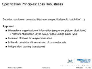
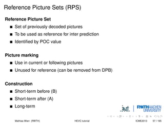
![Reference Picture Sets
Short-term and long-term reference pictures
Signaling
Short-term reference picture sets
Pictures in the proximity of the current picture
List of usable short-term RPSs in Sequence Parameter Set (SPS)
Alternative: explicit signaling in slice segment header
Slice indicates which predefined RPS to apply
Long-term reference picture set
Signaled in SPS
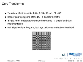
Alternative: explicit signaling in slice segment header
further reading: [14]
Mathias Wien (RWTH) HEVC tutorial ICME2013 58 / 165](https://image.slidesharecdn.com/tutorialhighefficiencyvideocodingcoding-toolsandspecification-221218095016-665f1135/85/Tutorial-High-Efficiency-Video-Coding-Coding-Tools-and-Specification-pdf-58-320.jpg)
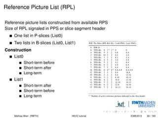
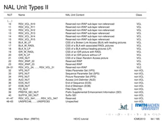
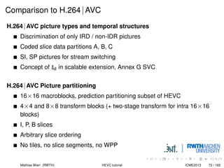
![Short-Term RPS – Example
POC
RPS
8
B0 *
B1
B2
B3
0 8
4
2 6
1 3 5 7
-1
-2
-3
-4
-5
-6
-7
-8
9
B0 A0
*
B1
10
B0 A1
A0
*
B1
3
B0 A2
A1
A0
*
4
B1 A1
A0
B0 *
5
B2 A0
B0
B1 *
6
B1 A1
B0 A0
*
7
B2 A0
B1 B0 *
0 8
4
2 6
1 3 5 7
-1
-2
-3
-4
-5
-6
-7
-8
RPS of random access configuration from the JCT-VC
common testing conditions JCTVC-K1100 [15]
Mathias Wien (RWTH) HEVC tutorial ICME2013 59 / 165](https://image.slidesharecdn.com/tutorialhighefficiencyvideocodingcoding-toolsandspecification-221218095016-665f1135/85/Tutorial-High-Efficiency-Video-Coding-Coding-Tools-and-Specification-pdf-59-320.jpg)
![Short-Term RPS – Example
POC
RPS
0 8
B0 *
B1
B2
B3
0 8
4
2 6
1 3 5 7
-1
-2
-3
-4
-5
-6
-7
-8
1 9
B0 A0
*
B1
2 10
B0 A1
A0
*
B1
3
B0 A2
A1
A0
*
4
B1 A1
A0
B0 *
5
B2 A0
B0
B1 *
6
B1 A1
B0 A0
*
7
B2 A0
B1 B0 *
0 8
4
2 6
1 3 5 7
-1
-2
-3
-4
-5
-6
-7
-8
RPS of random access configuration from the JCT-VC
common testing conditions JCTVC-K1100 [15]
Mathias Wien (RWTH) HEVC tutorial ICME2013 59 / 165](https://image.slidesharecdn.com/tutorialhighefficiencyvideocodingcoding-toolsandspecification-221218095016-665f1135/85/Tutorial-High-Efficiency-Video-Coding-Coding-Tools-and-Specification-pdf-60-320.jpg)
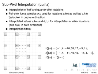
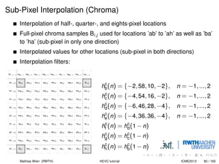
![Sub-Pixel Interpolation Filter Derivation
p−3 p−2 p−1 p0 p1 p2 p3 p4
pδ
δ
DCT-based interpolation filter
Interpolation filter derived from inverse DCT at shifted pixel location pδ
Forward and inverse DCT in one filter operation
Additional weighted window functions for reduction of ripple in filter
frequency response
Derivation scheme applicable for arbitrary sub-pixel locations
e. g. JCTVC-D344 [16], JCTVC-F247 [17]
Mathias Wien (RWTH) HEVC tutorial ICME2013 81 / 165](https://image.slidesharecdn.com/tutorialhighefficiencyvideocodingcoding-toolsandspecification-221218095016-665f1135/85/Tutorial-High-Efficiency-Video-Coding-Coding-Tools-and-Specification-pdf-82-320.jpg)


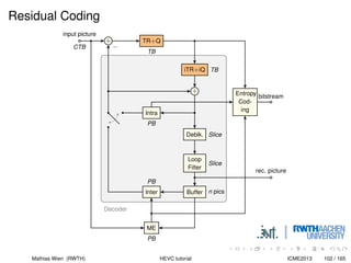
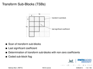
![Coded Representation of Transform Blocks
Coded transform coefficient information in five scan passes
Significance map
Level larger than 1
Level larger than 2
Coefficient sign
Remaining absolute level
Level larger than 1 and 2 scans terminate early if too many significant
coefficients
SoJoNgJiKaClHeDu12 [19]
Mathias Wien (RWTH) HEVC tutorial ICME2013 114 / 165](https://image.slidesharecdn.com/tutorialhighefficiencyvideocodingcoding-toolsandspecification-221218095016-665f1135/85/Tutorial-High-Efficiency-Video-Coding-Coding-Tools-and-Specification-pdf-121-320.jpg)
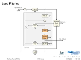
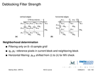
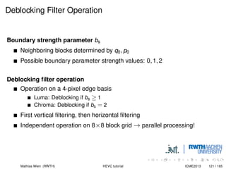
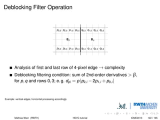
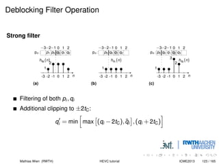
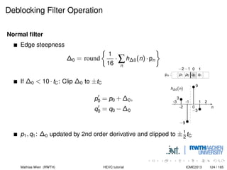
![Deblocking Filter
Design considerations
Reduction of visible blocking artifacts from block-wise processing
Computational complexity
Parallel processing
H.264|AVC deblocking filter in comparison:
Operation on 4×4 block boundary grid
Operation on macroblock basis (no parallel processing)
Higher computational complexity
[20]
Mathias Wien (RWTH) HEVC tutorial ICME2013 119 / 165](https://image.slidesharecdn.com/tutorialhighefficiencyvideocodingcoding-toolsandspecification-221218095016-665f1135/85/Tutorial-High-Efficiency-Video-Coding-Coding-Tools-and-Specification-pdf-126-320.jpg)
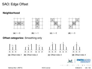
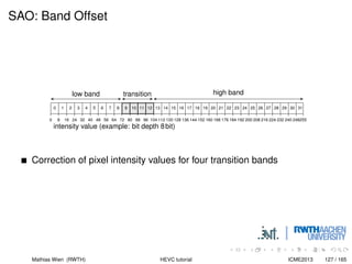
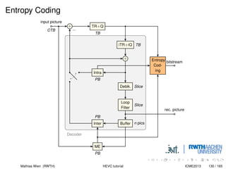
![Sample Adaptive Offset (SAO)
New filter type in ITU-T / MPEG video coding specifications
Local processing of pixels
Depending on local neighborhood, or
Depending on pixel value (amplitude)
Operation independent of processed pixels → parallel processing
Local filter parameter adaptation
[21]
Mathias Wien (RWTH) HEVC tutorial ICME2013 125 / 165](https://image.slidesharecdn.com/tutorialhighefficiencyvideocodingcoding-toolsandspecification-221218095016-665f1135/85/Tutorial-High-Efficiency-Video-Coding-Coding-Tools-and-Specification-pdf-132-320.jpg)

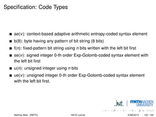
![CABAC
Context-based Adaptive Binary Arithmetic Coding
Binary Arithmetic Coder
syntax element
Binarizer
Context
Modeler
Adaptive
Engine
Bypass
Engine
bitstream
bin string
binary value
bin value coded bits
bin value coded bits
context update
MaScWi03 [22]
Mathias Wien (RWTH) HEVC tutorial ICME2013 134 / 165](https://image.slidesharecdn.com/tutorialhighefficiencyvideocodingcoding-toolsandspecification-221218095016-665f1135/85/Tutorial-High-Efficiency-Video-Coding-Coding-Tools-and-Specification-pdf-141-320.jpg)
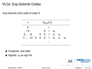
![CABAC State Transition
0 5 10 15 20 25 30 35 40 45 50 55 60
0.1
0.2
0.3
0.4
0.5
p̃LPSi
ipLPS
state ipLPS
state ipLPS
+1
LPS
MPS
State transitions ipLPS
= 0...62
State ipLPS
= 63 for termination
Highest value p̃LPSi = 0.5 for ipLPS
= 0
Change of vMPS if coding LPS and ipLPS
= 0
MaScWi03 [22]
Mathias Wien (RWTH) HEVC tutorial ICME2013 136 / 165](https://image.slidesharecdn.com/tutorialhighefficiencyvideocodingcoding-toolsandspecification-221218095016-665f1135/85/Tutorial-High-Efficiency-Video-Coding-Coding-Tools-and-Specification-pdf-143-320.jpg)
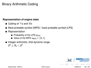
![CABAC Throughput
Reduced number of bins using context adaptation: Less computational
complexity for bypass coded bins (range adaptation by bit shift)
Grouping of bypass bins
Grouping of bins with same context
Minimized context dependencies
Avoidance of parsing dependencies
SzBu12 [11]
Mathias Wien (RWTH) HEVC tutorial ICME2013 142 / 165](https://image.slidesharecdn.com/tutorialhighefficiencyvideocodingcoding-toolsandspecification-221218095016-665f1135/85/Tutorial-High-Efficiency-Video-Coding-Coding-Tools-and-Specification-pdf-149-320.jpg)
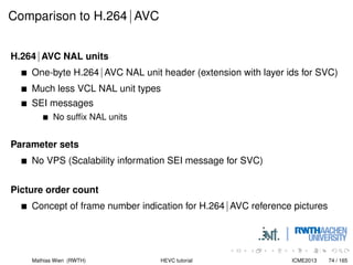
![Comparison to H.264|AVC
Reduced total number of coded bins (worst case, 1.5×)
Reduced number of context coded bins (8×)
Reduced number of contexts, storage size: 153 for HEVC, 459 (289 w/o
interlaced) for H.264|AVC. 8 bit initialization values in HEVC, 16 bit in
H.264|AVC
Coefficient memory consumption: 4×4 transform sub-blocks
Cleaner structure
Grouping of bypass bins, bins with same context
Reduced parsing dependencies (without significant performance impact)
SzBu12 [11]
Mathias Wien (RWTH) HEVC tutorial ICME2013 143 / 165](https://image.slidesharecdn.com/tutorialhighefficiencyvideocodingcoding-toolsandspecification-221218095016-665f1135/85/Tutorial-High-Efficiency-Video-Coding-Coding-Tools-and-Specification-pdf-150-320.jpg)

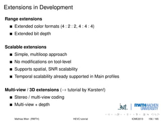
![HEVC Compression Performance
Significantly improved compression performance
Comparison of H.264|AVC and HEVC
Subjective and objective quality assessment: OhSuHeTaWi12 [3]
Complexity analysis: BoBrSuFl12 [4]
Facts
Reportedly about 49% bitrate savings for HEVC compared to H.264|AVC
for entertainment application scenario [3]
HEVC real-time encoder and decoder implementations reported and
demonstrated at the JCT-VC meetings, e. g. JCTVC-L0098 [23],
JCTVC-L0379 [24]
Mathias Wien (RWTH) HEVC tutorial ICME2013 150 / 165](https://image.slidesharecdn.com/tutorialhighefficiencyvideocodingcoding-toolsandspecification-221218095016-665f1135/85/Tutorial-High-Efficiency-Video-Coding-Coding-Tools-and-Specification-pdf-157-320.jpg)
![Subjective Assessment Results
Entertainment applications
Figure from OhSuHeTaWi12 [3]
Mathias Wien (RWTH) HEVC tutorial ICME2013 151 / 165](https://image.slidesharecdn.com/tutorialhighefficiencyvideocodingcoding-toolsandspecification-221218095016-665f1135/85/Tutorial-High-Efficiency-Video-Coding-Coding-Tools-and-Specification-pdf-158-320.jpg)
![Subjective Assessment Results
Entertainment applications
Figure from OhSuHeTaWi12 [3]
Mathias Wien (RWTH) HEVC tutorial ICME2013 152 / 165](https://image.slidesharecdn.com/tutorialhighefficiencyvideocodingcoding-toolsandspecification-221218095016-665f1135/85/Tutorial-High-Efficiency-Video-Coding-Coding-Tools-and-Specification-pdf-159-320.jpg)
![Subjective Assessment Results
Entertainment applications
Figure from OhSuHeTaWi12 [3]
Mathias Wien (RWTH) HEVC tutorial ICME2013 153 / 165](https://image.slidesharecdn.com/tutorialhighefficiencyvideocodingcoding-toolsandspecification-221218095016-665f1135/85/Tutorial-High-Efficiency-Video-Coding-Coding-Tools-and-Specification-pdf-160-320.jpg)
![Subjective Assessment Results
Entertainment applications
Figure from OhSuHeTaWi12 [3]
Mathias Wien (RWTH) HEVC tutorial ICME2013 154 / 165](https://image.slidesharecdn.com/tutorialhighefficiencyvideocodingcoding-toolsandspecification-221218095016-665f1135/85/Tutorial-High-Efficiency-Video-Coding-Coding-Tools-and-Specification-pdf-161-320.jpg)


![References I
[1] High efficiency video coding. ITU-T Recommendation H.265 and ISO/IEC 23008-2 (HEVC). Apr. 2013.
[2] Gary J. Sullivan et al. “Overview of the High Efficiency Video Coding (HEVC) Standard”. In: IEEE Transactions on Circuits and
Systems for Video Technology 22.12 (Dec. 2012), pp. 1649–1668. DOI: 10.1109/TCSVT.2012.2221191.
[3] Jens-Rainer Ohm et al. “Comparison of the Coding Efficiency of Video Coding Standards—Including High Efficiency Video Coding
(HEVC)”. In: IEEE Transactions on Circuits and Systems for Video Technology 22.12 (Dec. 2012), pp. 1669–1684. DOI:
10.1109/TCSVT.2012.2221192.
[4] Frank Bossen et al. “HEVC Complexity and Implementation Analysis”. In: IEEE Transactions on Circuits and Systems for Video
Technology 22.12 (Dec. 2012), pp. 1685–1696. DOI: 10.1109/TCSVT.2012.2221255.
[5] VCEG and MPEG. Terms of Reference of the Joint Collaborative Team on Video Coding Standard Development. Doc. VCEG-AM90.
Kyoto, JP: ITU-T SG16/Q6 VCEG, Jan. 2010.
[6] VCEG and MPEG. Joint Call for Proposals on Video Compression Technology. Doc. VCEG-AM91. Kyoto, JP: ITU-T SG16/Q6 VCEG,
Jan. 2010.
[7] Charles Poynton. Digital Video and HD: Algorithms and Interfaces. Waltham, MA, USA: Morgan Kaufman Publishers, 2012.
[8] Video codec for audiovisual services at p ×64kbit/s. ITU-T Recommendation H.261. 1993. URL:
http://www.itu.int/rec/T-REC-H.261/en.
[9] Gisle Bjontegaard. Calculation of average PSNR differences between RD curves. Doc. VCEG-M33. Austin, TX, USA: ITU-T SG16/Q6
VCEG, Apr. 2001.
[10] Jing Wang, Xiang Yu, and Dake He. On BD-rate calculation. Doc. JCTVC-F270. Torino, IT, 6th meeting: Joint Collaborative Team on
Video Coding (JCT-VC) of ITU-T VCEG and ISO/IEC MPEG, July 2011.
[11] Vivienne Sze and Madhukar Budagavi. “High Throughput CABAC Entropy Coding in HEVC”. In: IEEE Transactions on Circuits and
Systems for Video Technology 22.12 (Dec. 2012), pp. 1778–1791. DOI: 10.1109/TCSVT.2012.2221526.
[12] Madhukar Budagavi and Louis Kreofsky. BoG report on Quantization. Doc. JCTVC-G1044. Geneva, CH, 7th meeting: Joint
Collaborative Team on Video Coding (JCT-VC) of ITU-T VCEG and ISO/IEC MPEG, Nov. 2011.
Mathias Wien (RWTH) HEVC tutorial ICME2013 164 / 165](https://image.slidesharecdn.com/tutorialhighefficiencyvideocodingcoding-toolsandspecification-221218095016-665f1135/85/Tutorial-High-Efficiency-Video-Coding-Coding-Tools-and-Specification-pdf-171-320.jpg)
![References II
[13] Louis Kerofsky and Andrew Segall. Non CE4: Limiting dynamic range when using a quantization weighting matrix. Doc. JCTVC-H0541.
San Jose, CA, USA, 8th meeting: Joint Collaborative Team on Video Coding (JCT-VC) of ITU-T VCEG and ISO/IEC MPEG, Jan. 2012.
[14] Rickard Sjöberg et al. “Overview of HEVC high-level syntax and reference picture management”. In: IEEE Transactions on Circuits and
Systems for Video Technology 22.12 (Dec. 2012), pp. 1858–1870. DOI: 10.1109/TCSVT.2012.2223052.
[15] Frank Bossen. Common test conditions and software reference configurations. Doc. JCTVC-K1100. Shanghai, CN, 11th meeting: Joint
Collaborative Team on Video Coding (JCT-VC) of ITU-T VCEG and ISO/IEC MPEG, Oct. 2012.
[16] Elena Alshina et al. CE3: Experimental results of DCTIF by Samsung. Doc. JCTVC-D344. Daegu, KR, 4th meeting: Joint Collaborative
Team on Video Coding (JCT-VC) of ITU-T VCEG and ISO/IEC MPEG, Jan. 2011.
[17] Elena Alshina and Alexander Alshin. CE3: DCT derived interpolation filter test by Samsung. Doc. JCTVC-F247. Torino, IT, 6th meeting:
Joint Collaborative Team on Video Coding (JCT-VC) of ITU-T VCEG and ISO/IEC MPEG, July 2011.
[18] Jani Lainema et al. “Intra Coding of the HEVC Standard”. In: IEEE Transactions on Circuits and Systems for Video Technology 22.12
(Dec. 2012), pp. 1792–1801. DOI: 10.1109/TCSVT.2012.2221525.
[19] Joel Sole et al. “Transform Coefficient Coding in HEVC”. In: IEEE Transactions on Circuits and Systems for Video Technology 22.12
(Dec. 2012), pp. 1765–1777. DOI: 10.1109/TCSVT.2012.2223055.
[20] Andrey Norkin et al. “HEVC Deblocking Filter”. In: IEEE Transactions on Circuits and Systems for Video Technology 22.12 (Dec. 2012),
pp. 1746–1754. DOI: 10.1109/TCSVT.2012.2223053.
[21] Chih-Ming Fu et al. “Sample Adaptive Offset in the HEVC Standard”. In: IEEE Transactions on Circuits and Systems for Video
Technology 22.12 (Dec. 2012), pp. 1755–1764. DOI: 10.1109/TCSVT.2012.2221529.
[22] Detlev Marpe, Heiko Schwarz, and Thomas Wiegand. “Context-Based Adaptive Binary Arithmetic Coding in the H.264/AVC Video
Compression Standard”. In: IEEE Transactions on Circuits and Systems for Video Technology 13.7 (July 2003), pp. 620–637.
[23] Thiow K. Tan, Yoshinori Suzuki, and Frank Bossen. On software complexity: decoding 4K60p content on a laptop. Doc. JCTVC-L0098.
Geneva, CH, 12th meeting: Joint Collaborative Team on Video Coding (JCT-VC) of ITU-T VCEG and ISO/IEC MPEG, Jan. 2013.
[24] A. Minezawa et al. HEVC Real-time Hardware Encoder for HDTV signal. Doc. JCTVC-L0379. Geneva, CH, 12th meeting: Joint
Collaborative Team on Video Coding (JCT-VC) of ITU-T VCEG and ISO/IEC MPEG, Jan. 2013.
Mathias Wien (RWTH) HEVC tutorial ICME2013 165 / 165](https://image.slidesharecdn.com/tutorialhighefficiencyvideocodingcoding-toolsandspecification-221218095016-665f1135/85/Tutorial-High-Efficiency-Video-Coding-Coding-Tools-and-Specification-pdf-172-320.jpg)


![[IJET-V1I2P1] Authors :Imran Ullah Khan ,Mohd. Javed Khan ,S.Hasan Saeed ,Nup...](https://cdn.slidesharecdn.com/ss_thumbnails/ijet-v1i2p1-150413013648-conversion-gate01-thumbnail.jpg?width=640&height=640&fit=bounds)