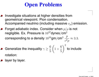
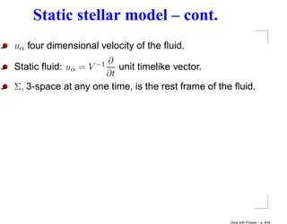
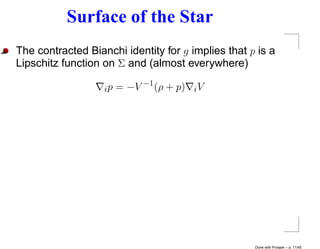
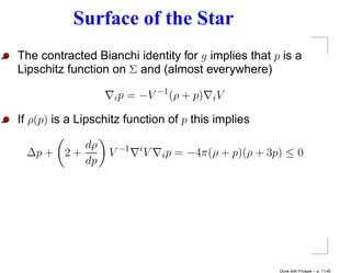
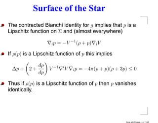
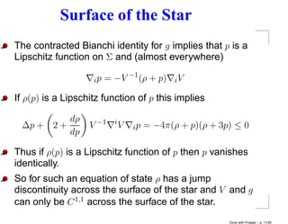
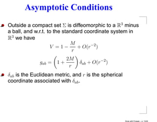
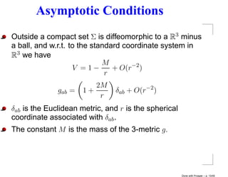
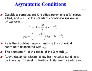
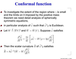
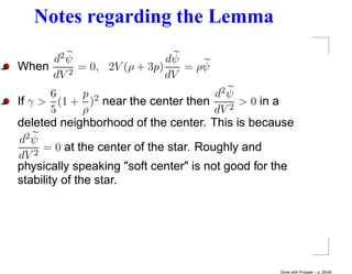
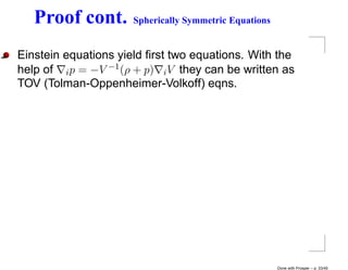
The document discusses the properties of static stellar models described by Einstein's equations. It defines key terms like the equation of state, adiabatic index, pressure, and density. It describes the conditions imposed on the metric, pressure, and density functions. The boundary of the star is defined as the surface where pressure goes to zero, and must be a smooth surface. Outside the star, the metric and potential are required to approach the Schwarzschild solution asymptotically.

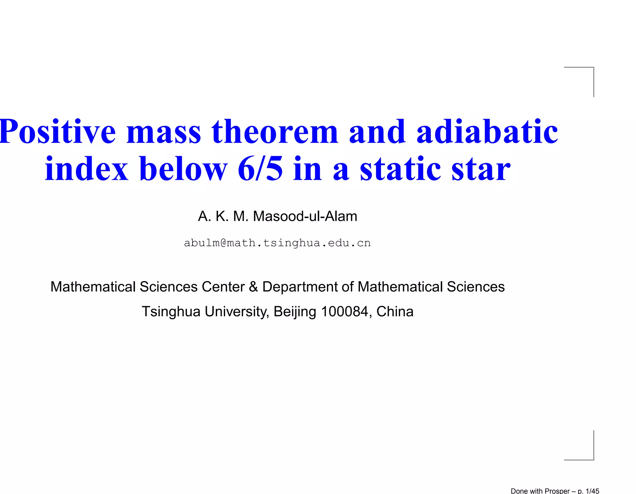


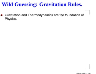
![p is a Function of V
We write i p = −V −1 (ρ + p) iV in the form
dp
= −V −1 (ρ + p)
dV
Thus the boundary of the star is a level set of V
henceforth dentoted by V = VS .
Since we assumed ρ to be a piecewise C 1 function of p
for p > 0,
ρ = ρ(V ) is also a piecewise C 1 function of V on [Vc , VS ].
Vc is the minimum value of V on Σ.
Done with Prosper – p. 12/45](https://image.slidesharecdn.com/tp-110705231720-phpapp02/85/Tp-42-320.jpg)
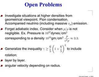
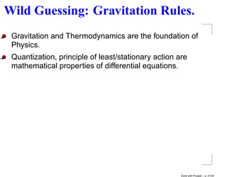
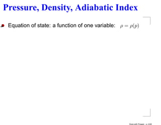
![Impossibilty of γ ≤ 6/5 Everywhere
1
Theorem [Lindblom, Masood-ul-Alam] Assume is
γ(p)
bounded as p → 0+ . Then γ must satisfy the inequality
2
6 p 6
γ> 1+ ≥
5 ρ 5
at some point inside a finite star.
Done with Prosper – p. 14/45](https://image.slidesharecdn.com/tp-110705231720-phpapp02/85/Tp-47-320.jpg)
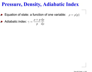
![Impossibilty of γ ≤ 6/5 Everywhere
1
Theorem [Lindblom, Masood-ul-Alam] Assume is
γ(p)
bounded as p → 0+ . Then γ must satisfy the inequality
2
6 p 6
γ> 1+ ≥
5 ρ 5
at some point inside a finite star.
Limits on the adiabatic index in static stellar models, in
B.L. Hu and T. Jacobson ed. Directions in General Relativity,
Cambridge University Press (1993).
Done with Prosper – p. 14/45](https://image.slidesharecdn.com/tp-110705231720-phpapp02/85/Tp-48-320.jpg)
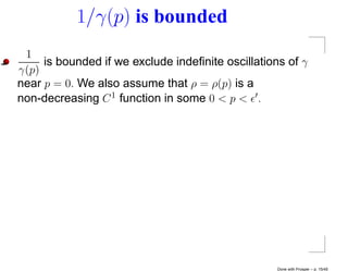
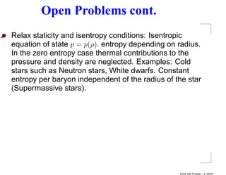
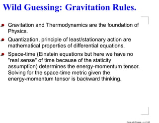
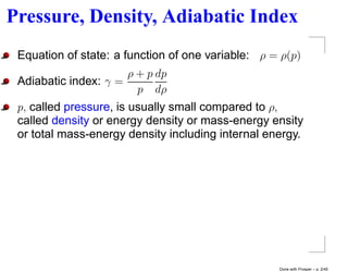
![1/γ(p) is bounded
1
is bounded if we exclude indefinite oscillations of γ
γ(p)
near p = 0. We also assume that ρ = ρ(p) is a
non-decreasing C 1 function in some 0 < p < .
Theorem [Lindblom, Masood-ul-Alam] γ(p) > 1 at some
point in every open interval (0, ).
Done with Prosper – p. 15/45](https://image.slidesharecdn.com/tp-110705231720-phpapp02/85/Tp-50-320.jpg)
![1/γ(p) is bounded
1
is bounded if we exclude indefinite oscillations of γ
γ(p)
near p = 0. We also assume that ρ = ρ(p) is a
non-decreasing C 1 function in some 0 < p < .
Theorem [Lindblom, Masood-ul-Alam] γ(p) > 1 at some
point in every open interval (0, ).
In particular if the equation of state is nice enough such
1
that lim inf γ(p) = lim sup γ(p) then is bounded on
p↓0 +
p↓0+ γ(p)
(0, pc ].
Done with Prosper – p. 15/45](https://image.slidesharecdn.com/tp-110705231720-phpapp02/85/Tp-51-320.jpg)

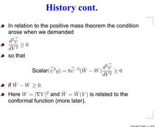
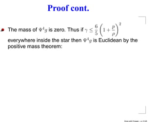
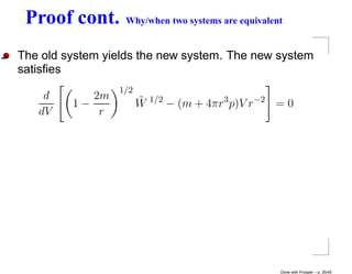
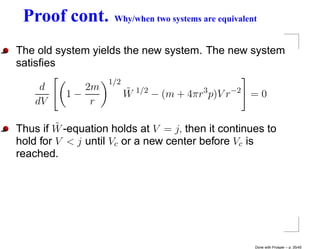
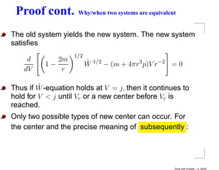
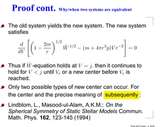
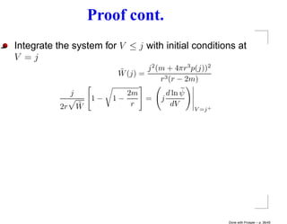
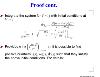
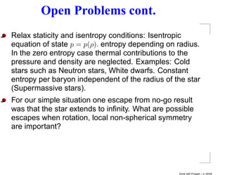
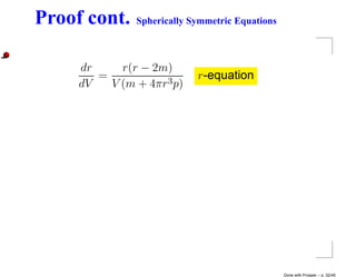
![Proof cont.
2
6 p
The mass of Ψ4 gis zero. Thus if γ ≤ 1+
5 ρ
everywhere inside the star then Ψ4 g is Euclidean by the
positive mass theorem:
Theorem [Schoen, Yau] Let (N, η) be a complete oriented
3-dimensional Riemannian manifold. Suppose (N, η) is
asymptotically flat and has non-negative scalar
curvature. Then the mass of (N.η) is non-negative and
if the mass is zero then (N, η) is isometric to R3 with the
standard euclidean metric.
Done with Prosper – p. 21/45](https://image.slidesharecdn.com/tp-110705231720-phpapp02/85/Tp-70-320.jpg)
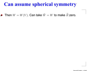
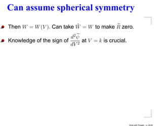
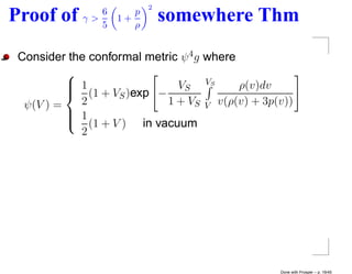
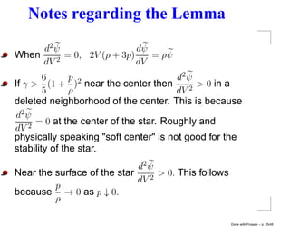
![Can assume spherical symmetry
˜
Then W = W (V ). Can take W = W to make R zero.
d2 ψ
Knowledge of the sign of 2
at V = k is crucial.
dV
d2 ψ
Lemma At V < VS where 2
= 0 and ψ(V ) is thrice
dV
differentiable, we have
d3 ψ 5πρ2 ψ 6 p 2
= [γ − (1 + ) ]
dV 3
γW˜ V (ρ + 3p) 5 ρ
Done with Prosper – p. 24/45](https://image.slidesharecdn.com/tp-110705231720-phpapp02/85/Tp-81-320.jpg)
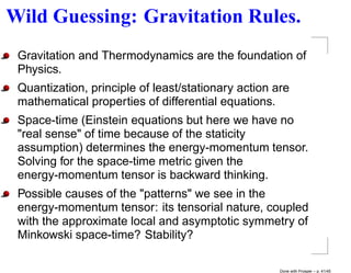
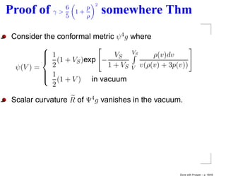
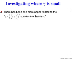
![Extent of the region where γ is small
Theorem [Masood-ul-Alam] There cannot be an interval
2
6 p
j < V < k inside a finite star where γ < 1+
5 ρ
Done with Prosper – p. 26/45](https://image.slidesharecdn.com/tp-110705231720-phpapp02/85/Tp-85-320.jpg)
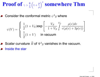
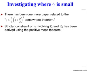
![Extent of the region where γ is small
Theorem [Masood-ul-Alam] There cannot be an interval
2
6 p
j < V < k inside a finite star where γ < 1+
5 ρ
d2 ψ
if 2
≥ 0 at V = k− .
dV
Done with Prosper – p. 26/45](https://image.slidesharecdn.com/tp-110705231720-phpapp02/85/Tp-86-320.jpg)
![Extent of the region where γ is small
Theorem [Masood-ul-Alam] There cannot be an interval
2
6 p
j < V < k inside a finite star where γ < 1+
5 ρ
d2 ψ
if 2
≥ 0 at V = k− .
dV
d2 ψ
if 2
< 0 at V = k− and ... ? ...
dV
Done with Prosper – p. 26/45](https://image.slidesharecdn.com/tp-110705231720-phpapp02/85/Tp-87-320.jpg)
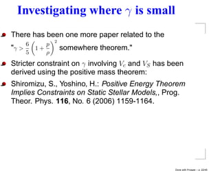
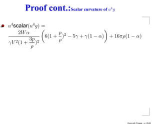
![Extent of the region where γ is small
Theorem [Masood-ul-Alam] There cannot be an interval
2
6 p
j < V < k inside a finite star where γ < 1+
5 ρ
d2 ψ
if 2
≥ 0 at V = k− .
dV
d2 ψ
if 2
< 0 at V = k− and ... ? ...
dV
k− allows ρ to be discontinuous at k.
Done with Prosper – p. 26/45](https://image.slidesharecdn.com/tp-110705231720-phpapp02/85/Tp-88-320.jpg)
![Proof
Choose a conformal function u(V ) on [j, k] that matches
at V = k in a C 1,1 fashion and gives positive scalar
curvature on [j, k] as before. Then if
Done with Prosper – p. 27/45](https://image.slidesharecdn.com/tp-110705231720-phpapp02/85/Tp-89-320.jpg)
![Proof
Choose a conformal function u(V ) on [j, k] that matches
at V = k in a C 1,1 fashion and gives positive scalar
curvature on [j, k] as before. Then if
d ln u
0 < 2j < 1,
dV V =j+
we can construct portion of a new star solving the
spherically symmetric equations with appopriate initial
˜
conditions at V = j. The new pair (W , ψ) makes the
metric ψ 4 g scalar flat in this portion.
Done with Prosper – p. 27/45](https://image.slidesharecdn.com/tp-110705231720-phpapp02/85/Tp-90-320.jpg)
![Proof
Choose a conformal function u(V ) on [j, k] that matches
at V = k in a C 1,1 fashion and gives positive scalar
curvature on [j, k] as before. Then if
d ln u
0 < 2j < 1,
dV V =j+
we can construct portion of a new star solving the
spherically symmetric equations with appopriate initial
˜
conditions at V = j. The new pair (W , ψ) makes the
metric ψ 4 g scalar flat in this portion.
d2 ψ
If 2
≥ 0 at V = k− , the above condition is satisfied.
dV
Done with Prosper – p. 27/45](https://image.slidesharecdn.com/tp-110705231720-phpapp02/85/Tp-91-320.jpg)
![Proof
Choose a conformal function u(V ) on [j, k] that matches
at V = k in a C 1,1 fashion and gives positive scalar
curvature on [j, k] as before. Then if
d ln u
0 < 2j < 1,
dV V =j+
we can construct portion of a new star solving the
spherically symmetric equations with appopriate initial
˜
conditions at V = j. The new pair (W , ψ) makes the
metric ψ 4 g scalar flat in this portion.
d2 ψ
If 2
≥ 0 at V = k− , the above condition is satisfied.
dV
Done with Prosper – p. 27/45](https://image.slidesharecdn.com/tp-110705231720-phpapp02/85/Tp-92-320.jpg)
![Proof
Choose a conformal function u(V ) on [j, k] that matches
at V = k in a C 1,1 fashion and gives positive scalar
curvature on [j, k] as before. Then if
d ln u
0 < 2j < 1,
dV V =j+
we can construct portion of a new star solving the
spherically symmetric equations with appopriate initial
˜
conditions at V = j. The new pair (W , ψ) makes the
metric ψ 4 g scalar flat in this portion.
d2 ψ
If 2
≥ 0 at V = k− , the above condition is satisfied.
dV
Done with Prosper – p. 27/45](https://image.slidesharecdn.com/tp-110705231720-phpapp02/85/Tp-93-320.jpg)
![Proof
Choose a conformal function u(V ) on [j, k] that matches
at V = k in a C 1,1 fashion and gives positive scalar
curvature on [j, k] as before. Then if
d ln u
0 < 2j < 1,
dV V =j+
we can construct portion of a new star solving the
spherically symmetric equations with appopriate initial
˜
conditions at V = j. The new pair (W , ψ) makes the
metric ψ 4 g scalar flat in this portion.
d2 ψ
If 2
≥ 0 at V = k− , the above condition is satisfied.
dV
Done with Prosper – p. 27/45](https://image.slidesharecdn.com/tp-110705231720-phpapp02/85/Tp-94-320.jpg)
![Proof cont.: Conformal functions on [j, k]
k ρ(s)ds
−α
u(V ) = ψ(k)e V 2s(ρ(s) + 3p(s))
Done with Prosper – p. 28/45](https://image.slidesharecdn.com/tp-110705231720-phpapp02/85/Tp-95-320.jpg)
![Proof cont.: Conformal functions on [j, k]
k ρ(s)ds
−α
u(V ) = ψ(k)e V 2s(ρ(s) + 3p(s))
3p(k) d ln ψ
with constant α = 2k 1 +
ρ(k− ) dV
V =k
Done with Prosper – p. 28/45](https://image.slidesharecdn.com/tp-110705231720-phpapp02/85/Tp-96-320.jpg)
![Proof cont.: Conformal functions on [j, k]
k ρ(s)ds
−α
u(V ) = ψ(k)e V 2s(ρ(s) + 3p(s))
3p(k) d ln ψ
with constant α = 2k 1 +
ρ(k− ) dV
V =k
u satisfies
d ln u αρ
2V =
dV ρ + 3p
Done with Prosper – p. 28/45](https://image.slidesharecdn.com/tp-110705231720-phpapp02/85/Tp-97-320.jpg)
![Proof cont.: Conformal functions on [j, k]
k ρ(s)ds
−α
u(V ) = ψ(k)e V 2s(ρ(s) + 3p(s))
3p(k) d ln ψ
with constant α = 2k 1 +
ρ(k− ) dV
V =k
u satisfies
d ln u αρ
2V =
dV ρ + 3p
u matches with ψ at V = k in a C 1,1 fashion.
Done with Prosper – p. 28/45](https://image.slidesharecdn.com/tp-110705231720-phpapp02/85/Tp-98-320.jpg)
![Proof cont.: Conformal functions on [j, k]
k ρ(s)ds
−α
u(V ) = ψ(k)e V 2s(ρ(s) + 3p(s))
3p(k) d ln ψ
with constant α = 2k 1 +
ρ(k− ) dV
V =k
u satisfies
d ln u αρ
2V =
dV ρ + 3p
u matches with ψ at V = k in a C 1,1 fashion.
d ln u
α ≤ 1 =⇒ 0 < 2j <1
dV V =j+
Done with Prosper – p. 28/45](https://image.slidesharecdn.com/tp-110705231720-phpapp02/85/Tp-99-320.jpg)
![Proof cont.:Conformal functions on [j, k]
d2 ψ 2π dψ
Recall, = ρψ − 2V (ρ + 3p)
dV 2
W˜ dV
2πρψ 3p d ln ψ
= 1 − 2V 1+
W˜ ρ dV
Done with Prosper – p. 29/45](https://image.slidesharecdn.com/tp-110705231720-phpapp02/85/Tp-100-320.jpg)
![Proof cont.:Conformal functions on [j, k]
d2 ψ 2π dψ
Recall, = ρψ − 2V (ρ + 3p)
dV 2
W˜ dV
2πρψ 3p d ln ψ
= 1 − 2V 1+
W˜ ρ dV
d2 ψ 2π ψρ−
= (1 − α)
dV 2 W˜
V =k−
Done with Prosper – p. 29/45](https://image.slidesharecdn.com/tp-110705231720-phpapp02/85/Tp-101-320.jpg)
![Proof cont.:Conformal functions on [j, k]
d2 ψ 2π dψ
Recall, = ρψ − 2V (ρ + 3p)
dV 2
W˜ dV
2πρψ 3p d ln ψ
= 1 − 2V 1+
W˜ ρ dV
d2 ψ 2π ψρ−
= (1 − α)
dV 2 W˜
V =k−
d2 ψ
Thus if ≥ 0, α ≤ 1 and hence
dV 2
V =k−
Done with Prosper – p. 29/45](https://image.slidesharecdn.com/tp-110705231720-phpapp02/85/Tp-102-320.jpg)
![Proof cont.:Conformal functions on [j, k]
d2 ψ 2π dψ
Recall, = ρψ − 2V (ρ + 3p)
dV 2
W˜ dV
2πρψ 3p d ln ψ
= 1 − 2V 1+
W˜ ρ dV
d2 ψ 2π ψρ−
= (1 − α)
dV 2 W˜
V =k−
d2 ψ
Thus if ≥ 0, α ≤ 1 and hence
dV 2
V =k−
d ln u
0< < 1 which allows us to continue inward.
dV V =j+
Done with Prosper – p. 29/45](https://image.slidesharecdn.com/tp-110705231720-phpapp02/85/Tp-103-320.jpg)
![Proof cont.
A detailed analysis of the spherically symmetric
equations are necessary to ensure
Proof goes through even if for new star W becomes
zero early?
ψ matches at V = j in C 1,1 fashion.
ψ > 0.
On an interval [a, b] we shall denote by r = r(V ),
2
m = m(V ), W ˜ = W (V ) ≡ 1 − 2m
˜ dr
, and
r dV
ψ = ψ(V ) to be the solutions of the following equations
with initial values of the functions specified at j :
Done with Prosper – p. 31/45](https://image.slidesharecdn.com/tp-110705231720-phpapp02/85/Tp-106-320.jpg)
![Proof cont.
A detailed analysis of the spherically symmetric
equations are necessary to ensure
Proof goes through even if for new star W becomes
zero early?
ψ matches at V = j in C 1,1 fashion.
ψ > 0.
On an interval [a, b] we shall denote by r = r(V ),
2
m = m(V ), W ˜ = W (V ) ≡ 1 − 2m
˜ dr
, and
r dV
ψ = ψ(V ) to be the solutions of the following equations
with initial values of the functions specified at j :
Done with Prosper – p. 31/45](https://image.slidesharecdn.com/tp-110705231720-phpapp02/85/Tp-107-320.jpg)
![Proof cont.
A detailed analysis of the spherically symmetric
equations are necessary to ensure
Proof goes through even if for new star W becomes
zero early?
ψ matches at V = j in C 1,1 fashion.
ψ > 0.
On an interval [a, b] we shall denote by r = r(V ),
2
m = m(V ), W ˜ = W (V ) ≡ 1 − 2m
˜ dr
, and
r dV
ψ = ψ(V ) to be the solutions of the following equations
with initial values of the functions specified at j :
Done with Prosper – p. 31/45](https://image.slidesharecdn.com/tp-110705231720-phpapp02/85/Tp-108-320.jpg)
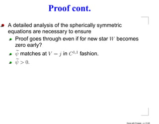
![Proof cont.
A detailed analysis of the spherically symmetric
equations are necessary to ensure
Proof goes through even if for new star W becomes
zero early?
ψ matches at V = j in C 1,1 fashion.
ψ > 0.
On an interval [a, b] we shall denote by r = r(V ),
2
m = m(V ), W ˜ = W (V ) ≡ 1 − 2m
˜ dr
, and
r dV
ψ = ψ(V ) to be the solutions of the following equations
with initial values of the functions specified at j :
Done with Prosper – p. 31/45](https://image.slidesharecdn.com/tp-110705231720-phpapp02/85/Tp-109-320.jpg)
![Proof cont. A new system of ODEs
Theorem [Lindblom,Masood-ul-Alam] ˜
If r(V ), m(V ), W (V )
˜
is a solution of the following system, r > 2m > 0, W > 0,
and initially the values of the three functions are related
˜ ˜
by W -equation, then W -equation continues to hold
subsequently .
1/2
dr 2m ˜ −1/2
= 1− W
dV r
1/2
dm 2m ˜
2
= 4πρr 1 − W −1/2
dV r
dW˜
= 8πV (ρ + p) − 4V mr−3
dV
Done with Prosper – p. 34/45](https://image.slidesharecdn.com/tp-110705231720-phpapp02/85/Tp-117-320.jpg)
![Proof cont. A new system of ODEs
Theorem [Lindblom,Masood-ul-Alam] ˜
If r(V ), m(V ), W (V )
˜
is a solution of the following system, r > 2m > 0, W > 0,
and initially the values of the three functions are related
˜ ˜
by W -equation, then W -equation continues to hold
subsequently .
1/2
dr 2m ˜ −1/2
= 1− W
dV r
1/2
dm 2m ˜
2
= 4πρr 1 − W −1/2
dV r
dW˜
= 8πV (ρ + p) − 4V mr−3
dV
Done with Prosper – p. 34/45](https://image.slidesharecdn.com/tp-110705231720-phpapp02/85/Tp-118-320.jpg)
![Proof cont. A new system of ODEs
Theorem [Lindblom,Masood-ul-Alam] ˜
If r(V ), m(V ), W (V )
˜
is a solution of the following system, r > 2m > 0, W > 0,
and initially the values of the three functions are related
˜ ˜
by W -equation, then W -equation continues to hold
subsequently .
1/2
dr 2m ˜ −1/2
= 1− W
dV r
1/2
dm 2m ˜
2
= 4πρr 1 − W −1/2
dV r
dW˜
= 8πV (ρ + p) − 4V mr−3
dV
Done with Prosper – p. 34/45](https://image.slidesharecdn.com/tp-110705231720-phpapp02/85/Tp-119-320.jpg)