Download to read offline
![Vorticity generation
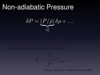
Vorticity can be sourced at second order from
non-adiabatic pressure:
ω2ij − Hω2ij ∝ δρ,[j δPnad,i]
˙
⇒ Vorticity can then source B-mode polarisation and/or
magnetic fields.
⇒ Possibly detectable in CMB.
Christopherson, Malik & Matravers 2009, 2011](https://image.slidesharecdn.com/talk-120328101424-phpapp01/85/Calculating-Non-adiabatic-Pressure-Perturbations-during-Multi-field-Inflation-9-320.jpg)

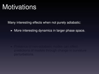
The document discusses the effects of non-adiabatic pressure perturbations during multi-field inflation, highlighting their impact on curvature perturbations and vorticity generation. It outlines the motivations for exploring non-adiabatic dynamics and reviews calculations and numerical results related to different inflationary models. The study includes software tools for further analysis and emphasizes caution in making predictions involving isocurvature modes at the end of inflation.


![Getting Started with Apache Spark: Big Data Made Simple [Free Meetup]](https://cdn.slidesharecdn.com/ss_thumbnails/apachesparkgettingstarted-260203175547-8361bcc3-thumbnail.jpg?width=640&height=640&fit=bounds)


