The document discusses inventory management and control techniques. It covers topics like setting stock levels, inventory budgeting, perpetual inventory systems, ABC analysis, economic order quantity (EOQ) modeling, and quantity discounts. ABC analysis involves categorizing inventory items into A, B, and C categories based on their value and accounting for 80%, 15-20%, and 5-10% of total spending, respectively. EOQ modeling determines the optimal order quantity to minimize total inventory costs based on factors like demand, ordering costs, and holding costs. Quantity discounts provide pricing incentives for purchasing higher volumes.

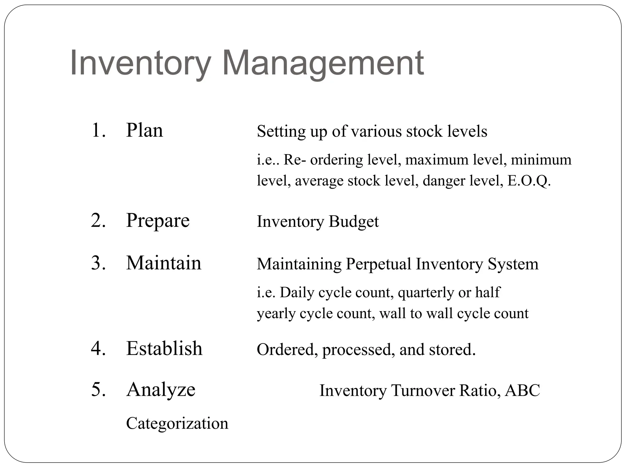
1. Lecture
IOBM
Inventory Control

2. Inventory Management
1. Plan Setting up of various stock levels
i.e.. Re- ordering level, maximum level, minimum
level, average stock level, danger level, E.O.Q.
2. Prepare Inventory Budget
3. Maintain Maintaining Perpetual Inventory System
i.e. Daily cycle count, quarterly or half
yearly cycle count, wall to wall cycle count
4. Establish Ordered, processed, and stored.
5. Analyze Inventory Turnover Ratio, ABC
Categorization

3. Inventory Classification
 ABC Analysis - Based on Pareto Principle i.e. 80/20
 HML Analysis – High, Medium and Low
 FSN Analysis - Fast, Slow , Non moving
 VED Analysis - Vital, Essential, Desirable

4. ABC Analysis
It is based on Pareto Principle i.e. 80/20;
“A” Category Items - Comprise 20% of SKU & Contribute to
75% - 80% of Rupee spend.
“B” Category Items - Comprise 30% of SKU & Contribute to
15% - 20% of Rupee spend.
“C” Category Items - Comprise 50% of SKU & Contribute to
5% -10% of Rupee spend.

5. ABC Analysis

6. Procedure for ABC Analysis
1. List each item carried in inventory by number or some other
designation.
2. Determine the annual volume of usage and rupee value of each item.
3. Multiply each item annual volume of usage by its rupee value.
4. Compute each item percentage of the total inventory in terms of
annual usage in rupees.
5. Select the top 20% of all items which have the highest rupee
percentages and classify them as “A” items.
6. Select the next 30% of all items with the next highest rupee
percentages and designate them as “B” items.
7. The next 50% of all items with the lowest rupee percentages are “C”
items.

7. Procedure for ABC Analysis
Step#1
S.No. Item number
Unit cost
($)
Annual demand
Total cost per year
($)
1 1001 6 48,000 288,000
2 1002 12 2,000 24,000
3 1003 20 300 6,000
4 1004 8 800 6,400
5 1005 7 4,800 33,600
6 1006 16 1,200 19,200
7 1007 18 18,000 324,000
8 1008 4 300 1,200
9 1009 9 5,000 45,000
10 1010 12 500 6,000
Total usage 753,400

8. S.No.
Item
number
Unit cost
($)
Annual demand
Total cost per year
($)
Usage as a %
of total usage
1 1001 6 48,000 288,000 38%
2 1002 12 2,000 24,000 3%
3 1003 20 300 6,000 1%
4 1004 8 800 6,400 1%
5 1005 7 4,800 33,600 4%
6 1006 16 1,200 19,200 3%
7 1007 18 18,000 324,000 43%
8 1008 4 300 1,200 0%
9 1009 9 5,000 45,000 6%
10 1010 12 500 6,000 1%
Total usage 753,400 100%
Procedure for ABC Analysis
Step#2

9. S.No. Category
Cumulative
% of items
Item
number
Unit
cost
Annual
demand
Total cost
per year
Usage as a
% of total
usage
Cumulative % of
total
1
A
10% 1007 18 18,000 324,000 43.0% 43.0%
2 20% 1001 6 48,000 288,000 38.2% 81.2%
3
B
30% 1009 9 5,000 45,000 6.0% 87.2%
4 40% 1005 7 4,800 33,600 4.5% 91.7%
5 50% 1002 12 2,000 24,000 3.2% 94.9%
6
C
60% 1006 16 1,200 19,200 2.5% 97.4%
7 70% 1004 8 800 6,400 0.8% 98.2%
8 80% 1010 12 500 6,000 0.8% 99.0%
9 90% 1003 20 300 6,000 0.8% 99.8%
10 100% 1008 4 300 1,200 0.2% 100%
Total Usage 753,400 100%
Procedure for ABC Analysis
Step#3

10. Economic Order Quantity (EOQ)
Economic Order Quantity Model determines the optimal order
Quantity that will minimize the total inventory cost.
This model pre supposes certain assumptions as under:
1. No safety Stocks available in inventory.
2. No shortages allowed in order delivery.
3. Demand is at uniform rate and does not fluctuate.
4. Lead Time for order delivery is constant.
5. The only two relevant costs are the inventory holding cost and the fixed
cost per lot for ordering or setup.
• EOQ is a basic model and further models developed based on this model e.g.
production Quantity Model and Quantity Discount Model.

11. Economic Order Quantity (Cont.)
Use the EOQ:
 Make-to-stock
 Carrying and setup costs are known and relatively stable
 Modify to quantity discounts

12. Economic Order Quantity (Cont.)

13. Calculating EOQ
• The EOQ Formula:
{D= Annual Demand, S= Set up or Ordering Cost, H= Holding Cost}
• Time Between Orders (TBO):
EOQ =
2DS
H
TBOEOQ = (12) months/year
EOQ
D

14. Calculating Cost - EOQ
Annual Holding Cost:
Annual holding cost = (Average cycle inventory)  (Unit holding cost)
Annual Ordering Cost:
Annual ordering cost = (Number of orders/Year)  (Ordering Cost)
Total Cost:
Total costs = Annual holding cost + Annual ordering or setup cost

15. Numerical Problem
Biotech. Co produces chemicals to sell to wholesalers. One of the raw
material it buys is sodium nitrate which is purchased at the rate of $22.50 per
ton. Biotech’s forecasts show a estimated requirement of 5,75,000 tons of
sodium nitrate for the coming year. The annual total carrying cost for this
material is 40% of purchase cost and the ordering cost is $595 per order.
What is the Most Economical Order Quantity and TBO?
Solution:
D= 5,75000 Tons, H= 22.50 x 40% = $9.00/Ton/Year, S = $595/Order
EOQ = =
2DS
H
= 27,573 tons per order
2(5,75000)(595
)
9
TBOEOQ = (12) months/year =
EOQ
D
27,573 (12) = 0.575 Month
575000

16. Numerical Problem
Suppose that you are reviewing the inventory policies on an $80 item
stocked at a hardware store. The current policy is to replenish
inventory by ordering in lots of 200 units. Additional information is;
D = 60 units per week, 60 x 52 = 3,120 units per year
S = $30 per order
H = 25% of selling price = 25% x $80 = $20 per unit per year
What is the EOQ?
EOQ = =
2DS
H = 97 units
2(3,120)(30)
20
SOLUTION

17. Application of EOQ
Current Policy EOQ Policy
Q = 200 Units EOQ = 97 Units
T.C = [Annual H.C] + [Annual S.C] T.C = [Annual H.C] + [Annual S.C]
T.C = [Avg. Cycle Inv. X Unit Holding Cost] + [No. Orders / Yr x Ordering Cost]
T.C = (200/2)(20) + (3,120/200)(30) T.C = (97/2)(20) + (3,120/97)(30)
T.C = 2000 + 468 T.C = 970 + 965
T.C = $2468 T.C = $1,935
What is the total annual cost of the current policy (Q = 200), and
how does it compare with the cost by using the EOQ?

18. Application of EOQ (Cont.)
What is the time between orders (TBO) for the current policy and the EOQ
policy, expressed in weeks?
TBO200 = (52 weeks per year) = 3.3 weeks
200
3,120
TBOEOQ = (52 weeks per year) = 1.6 weeks
97
3,120
SOLUTION
TBOEOQ = (12) months/year or 52 weeks/year
EOQ
D

19. Quantity Discounts
This adjustment offers buyers an incentive of lower per-unit
pricing as more products are purchased.
For instance, a buyer may pay the list price when they purchase between
1-99 units but receive a 5% discount off the list price when the purchase
exceeds 100 units.

20. Quantity Discounts Models
1. All units quantity discount
e.g. X amount of discount offer, if order quantity per annum > 2000
2. Incremental units quantity discount. Following is an example;
Total Annual Cost:
Quantity Discount Unit Price
1-999 units 0% $5.00
1000-1999 units 4% $4.80
2000 or more units 5% $4.75
TC = [ (Q/2) x H ] + [ (D/Q) x S ] + [ P x D ]
ANNUAL CARRYING COST ANNUAL ORDERING COST ANNUAL FIXED COST

21. Example
Annual Demand = 5,000 units
Ordering Cost = $49.00
Carrying Cost as Percentage of Unit Price = 20%
Package Offer;
Quantity Discount Unit Price H.C/Unit
1-999 units (Q1) 0% $5.00 0.20 x 5 = $1.00
1000-1999 units (Q2) 4% $4.80 0.20 x 4.80 = $0.96
2000 or more units (Q3) 5% $4.75 0.20 x 4.75 = $0.95

22. EOQ2 = = = 714 units (for 4% discount)
2DS
H
2x5000x49
0.96
( to qualify for the 0% discount )
EOQ1 = 700 need not be adjusted
( to qualify for the 4% discount )
EOQ2 = 714 is adjusted to EOQ2 = 1,000 units
( to qualify for the 5% discount )
EOQ3 = 718 is adjusted to EOQ3 = 2,000 units
EOQ1 = = = 700 units (for 0% discount)
2DS
H
2x5000x49
1
EOQ3 = = = 718 units (for 5% discount)
2DS
H
2x5000x49
0.95
Example (Cont.)

23. Total Cost:
Example (Cont.)
TC2 = [ (EOQ2/2) x H ] + [ (D/EOQ2) x S ] + [ P x D ]
TC2 = [ (1000/2) x 0.96] + [ (5000/1000) x 49] + [4.80 x 5000]
TC2 = $480 + $245 + $24,000 = $24,725
TC1 = [ (EOQ1/2) x H ] + [ (D/EOQ1) x S ] + [ P x D ]
TC1 = [ (700/2) x 1] + [ (5000/700) x 49 ] + [ 5 x 5000 ]
TC1 = $350 + $350 + $25,000 = $25,700
TC3 = [ (EOQ3/2) x H ] + [ (D/EOQ3) x S ] + [ P x D ]
TC3 = [ (2000/2) x 0.95] + [ (5000/2000) x 49] + [4.75 x 5000]
TC3 = $950 + $122.50 + $23,750 = $24,822.50
TC = [ (Q/2) x H ] + [ (D/Q) x S ] + [ P x D ]

24. Example (Cont.)
Quantity
Annual
Holding Cost
Annual
Ordering Cost
Annual Material
Cost
TOTAL
700 units
Q1 -(@
$0%)
$350.00 $350.00 $25,000.00 $25,700.00
1000 units
Q2 –(@
$4%)
$480.00 $245.00 $24,000.00 $24,725.00
2000 units
Q3 –(@
$5%)
$950.00 $122.50 $23,750.00 $24,822.50
Summary