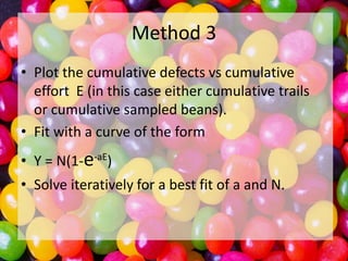
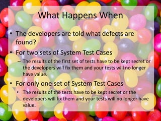
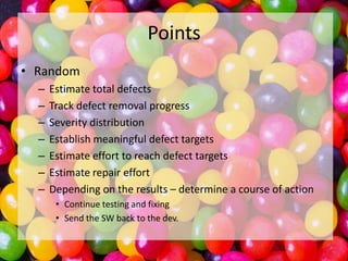
Jelly Beans
and
Software Verification
Introduction
• Tom Walton
• Software Quality Assurance Specialist
• tom_walton@videotron.ca
Verification
• The processes that are relevant are
– Serial Processes
• Document and Code Inspection
• Unit Test
• Integration Test

– Random Processes
• System Level Verification
Serial Processes
• Pieces are verified one at a time
• Opportunity for 100% Coverage
• Historical data used for
– Estimating total defects
– Severity of remaining defects
Instructions
•
•
•
•

Use the scoop to take a sample
Count the green jelly beans
Record the number of scoops
Record the number of green Jelly beans in
each scoop
• Plot data
– Cumulative Green vs Cumulative Sampled

• Make an estimate of the total number of green
jelly beans present.
Serial Jelly Beans
120
Cum Green
Trend
Actual

100
Cumulative Green

Linear (Cum Green)

y = 2.6442x
R² = 0.9569
80

60

40

20

0
0

5

10

15

20
Trial

25

30

35

40
Code Inspection
Integration Test
Integration Test Defect Trend
350

Cumulative Defects

300
250
200

150
100
74% of Planned Tests
28 of 34 Activities Reporting

50
0
0

500

1000

1500

Cumulative Total Effort (hr)

2000

2500

3000
Using the Data
Code Inspection Performance
30.00

Defect Density (Def/KLOC)

Avg.Def/KLOC
25.00

Act. Def/KLOC

Too Fast

20.00

Too Buggy

15.00

Tend to be large modules

Point 1
Point 2

10.00

Def/KLOC x LOCs/hr = Constant

5.00

0.00
0

100

200

300

400

500

600

700

Inspection Speed (LOCS/hr.)

Measure
Size (LOCS)
Inspection Rate(Locs/Hr)
Defect Rate(Def/Hr)
Defect Density (Def/KLOC)

Average Point 1 Point 2
800
800
78
229
267
0.206
1.43
1.33
3.65
6
5

• t The planning datameasures can establish acceptance criteria. level.
The inspection can be used to be calculated incomponent
acceptance criteria can be applied at the the review.
System Testing Is Random
• For Real Software
– Defects were inserted at random.
– We do not know where the defects are.
– Our tests execute random bits of code.
System Verification
• Verification is to show that the software was
correctly built
– are there any defects?

• By the time system verification starts, the
product is built.
• We should not find any defects – but we do.
• Question is --- How many defects are left?
Instructions
• Use the scoop to take a sample
• Count the green jelly beans and replace them
with purple jelly beans.
• Record the number of scoops
• Record the number of green Jelly beans in each
scoop
• Plot data
– Cumulative Green vs Cumulative Sampled

• Make estimate of the total number of green jelly
beans originally present until 25 samples were
taken.
Replacing Green With Grape
45
40

Cum Green
Trend

Cum Green

35
30
25
20
15
10
5
0
0

5

10

15
Trials

20

25

30
Repeat the Process
• Use the scoop to take a sample
• Count the green jelly and purple beans and replace
them both.
• Record the number of scoops
• Record the number of green and purple jelly beans in
each scoop
• Plot data
– Cumulative Purple Vs Cumulative Sampled
– Cumulative Green vs Cumulative Sampled
– Cumulative Purple and Green vs Cumulative Samples

• Continue until 25 samples were taken.
• Estimate Defects using extrapolation
Have we run out of purple?
50
Cum Green

40

Cum Purple

35
Cum Beans

45

Cum Total

30

Trend

25
20
15
10
5
0
0

5

10

15
Trials

20

25

30
Re-Estimate
• With jelly beans it is difficult to exactly repeat
a trial but with software you can.
• But we know how many purple jelly beans we
put in and how many are left.
• We have three estimating methods available.
Three Estimating Methods
• First Method
– Uses only the data from one set of tests – divide
the effort in half.

• Second Method
– Uses data from both sets of tests
– Problem: needs two test groups both developing
test cases starting from the same requirements

• Third Method
– Extrapolation from one set of tests
Method 1
• Equal test effort finds an equal fraction of the
defects remaining.
• First n trails => X green jelly beans
• Second n trials => Y green jelly beans
• X/N = Y/(N-X)
– where N = original number of green jelly beans.

• Solving N = X2/(X-Y)
Method 2
• First set n trails => replaced X green jelly beans
• Second set m trials => Y green jelly beans and
Z purple jelly beans.
• If Z is a representative fraction
• N = X/Z(Y+Z)
– where N = original number of green jelly beans.
– Have to keep X a secret.
Method 3
• Plot the cumulative defects vs cumulative
effort E (in this case either cumulative trails
or cumulative sampled beans).
• Fit with a curve of the form

• Y = N(1-e-aE)
• Solve iteratively for a best fit of a and N.
Some Added Estimates
• Make an estimate of the number of samples
required to find 99% of the green and purple
jelly beans.
• Plot the fraction of purple jelly beans vs
number of samples.
• What can we conclude from this data?
Equal Effort => Equal Fraction
90
80

Cum Beans

70
60
50
Cum Green

40

Cum Purple

30

Cum Total
Trend

20

Series5

10
0
0

20

40

60
Trials

80

100

120
What Happens When
• The developers are told what defects are
found?
• For two sets of System Test Cases
– The results of the first set of tests have to be kept secret or
the developers will fix them and your tests will no longer
have value.

• For only one set of System Test Cases
• The results of the tests have to be kept secret or the
developers will fix them and your tests will no longer have
value.
Toward Zero Defects
• Give the estimated defect load to the
developers. They have cheaper ways of
finding and fixing defects.
• Only test to get an estimate and give that
estimate to the developers.
• Only retest to re-do the estimate
• System test cases and automation costs a lot
of money and time – don’t throw this away.
POINTS
• Serial
– Produces straight line
– Estimate defect yield from phases with effort
estimate
– Severity distribution
– Estimate repair effort (based on history)
– Used to estimate future projects with same team
– With historical data to estimate total defects
Points
• Random
–
–
–
–
–
–
–

Estimate total defects
Track defect removal progress
Severity distribution
Establish meaningful defect targets
Estimate effort to reach defect targets
Estimate repair effort
Depending on the results – determine a course of action
• Continue testing and fixing
• Send the SW back to the dev.

Tom walton - Jelly Beans And Software Verification

  • 1.
  • 2.
    Introduction • Tom Walton •Software Quality Assurance Specialist • tom_walton@videotron.ca
  • 3.
    Verification • The processesthat are relevant are – Serial Processes • Document and Code Inspection • Unit Test • Integration Test – Random Processes • System Level Verification
  • 4.
    Serial Processes • Piecesare verified one at a time • Opportunity for 100% Coverage • Historical data used for – Estimating total defects – Severity of remaining defects
  • 5.
    Instructions • • • • Use the scoopto take a sample Count the green jelly beans Record the number of scoops Record the number of green Jelly beans in each scoop • Plot data – Cumulative Green vs Cumulative Sampled • Make an estimate of the total number of green jelly beans present.
  • 6.
    Serial Jelly Beans 120 CumGreen Trend Actual 100 Cumulative Green Linear (Cum Green) y = 2.6442x R² = 0.9569 80 60 40 20 0 0 5 10 15 20 Trial 25 30 35 40
  • 7.
  • 8.
    Integration Test Integration TestDefect Trend 350 Cumulative Defects 300 250 200 150 100 74% of Planned Tests 28 of 34 Activities Reporting 50 0 0 500 1000 1500 Cumulative Total Effort (hr) 2000 2500 3000
  • 9.
    Using the Data CodeInspection Performance 30.00 Defect Density (Def/KLOC) Avg.Def/KLOC 25.00 Act. Def/KLOC Too Fast 20.00 Too Buggy 15.00 Tend to be large modules Point 1 Point 2 10.00 Def/KLOC x LOCs/hr = Constant 5.00 0.00 0 100 200 300 400 500 600 700 Inspection Speed (LOCS/hr.) Measure Size (LOCS) Inspection Rate(Locs/Hr) Defect Rate(Def/Hr) Defect Density (Def/KLOC) Average Point 1 Point 2 800 800 78 229 267 0.206 1.43 1.33 3.65 6 5 • t The planning datameasures can establish acceptance criteria. level. The inspection can be used to be calculated incomponent acceptance criteria can be applied at the the review.
  • 10.
    System Testing IsRandom • For Real Software – Defects were inserted at random. – We do not know where the defects are. – Our tests execute random bits of code.
  • 11.
    System Verification • Verificationis to show that the software was correctly built – are there any defects? • By the time system verification starts, the product is built. • We should not find any defects – but we do. • Question is --- How many defects are left?
  • 12.
    Instructions • Use thescoop to take a sample • Count the green jelly beans and replace them with purple jelly beans. • Record the number of scoops • Record the number of green Jelly beans in each scoop • Plot data – Cumulative Green vs Cumulative Sampled • Make estimate of the total number of green jelly beans originally present until 25 samples were taken.
  • 13.
    Replacing Green WithGrape 45 40 Cum Green Trend Cum Green 35 30 25 20 15 10 5 0 0 5 10 15 Trials 20 25 30
  • 14.
    Repeat the Process •Use the scoop to take a sample • Count the green jelly and purple beans and replace them both. • Record the number of scoops • Record the number of green and purple jelly beans in each scoop • Plot data – Cumulative Purple Vs Cumulative Sampled – Cumulative Green vs Cumulative Sampled – Cumulative Purple and Green vs Cumulative Samples • Continue until 25 samples were taken. • Estimate Defects using extrapolation
  • 15.
    Have we runout of purple? 50 Cum Green 40 Cum Purple 35 Cum Beans 45 Cum Total 30 Trend 25 20 15 10 5 0 0 5 10 15 Trials 20 25 30
  • 16.
    Re-Estimate • With jellybeans it is difficult to exactly repeat a trial but with software you can. • But we know how many purple jelly beans we put in and how many are left. • We have three estimating methods available.
  • 17.
    Three Estimating Methods •First Method – Uses only the data from one set of tests – divide the effort in half. • Second Method – Uses data from both sets of tests – Problem: needs two test groups both developing test cases starting from the same requirements • Third Method – Extrapolation from one set of tests
  • 18.
    Method 1 • Equaltest effort finds an equal fraction of the defects remaining. • First n trails => X green jelly beans • Second n trials => Y green jelly beans • X/N = Y/(N-X) – where N = original number of green jelly beans. • Solving N = X2/(X-Y)
  • 19.
    Method 2 • Firstset n trails => replaced X green jelly beans • Second set m trials => Y green jelly beans and Z purple jelly beans. • If Z is a representative fraction • N = X/Z(Y+Z) – where N = original number of green jelly beans. – Have to keep X a secret.
  • 20.
    Method 3 • Plotthe cumulative defects vs cumulative effort E (in this case either cumulative trails or cumulative sampled beans). • Fit with a curve of the form • Y = N(1-e-aE) • Solve iteratively for a best fit of a and N.
  • 21.
    Some Added Estimates •Make an estimate of the number of samples required to find 99% of the green and purple jelly beans. • Plot the fraction of purple jelly beans vs number of samples. • What can we conclude from this data?
  • 22.
    Equal Effort =>Equal Fraction 90 80 Cum Beans 70 60 50 Cum Green 40 Cum Purple 30 Cum Total Trend 20 Series5 10 0 0 20 40 60 Trials 80 100 120
  • 23.
    What Happens When •The developers are told what defects are found? • For two sets of System Test Cases – The results of the first set of tests have to be kept secret or the developers will fix them and your tests will no longer have value. • For only one set of System Test Cases • The results of the tests have to be kept secret or the developers will fix them and your tests will no longer have value.
  • 24.
    Toward Zero Defects •Give the estimated defect load to the developers. They have cheaper ways of finding and fixing defects. • Only test to get an estimate and give that estimate to the developers. • Only retest to re-do the estimate • System test cases and automation costs a lot of money and time – don’t throw this away.
  • 25.
    POINTS • Serial – Producesstraight line – Estimate defect yield from phases with effort estimate – Severity distribution – Estimate repair effort (based on history) – Used to estimate future projects with same team – With historical data to estimate total defects
  • 26.
    Points • Random – – – – – – – Estimate totaldefects Track defect removal progress Severity distribution Establish meaningful defect targets Estimate effort to reach defect targets Estimate repair effort Depending on the results – determine a course of action • Continue testing and fixing • Send the SW back to the dev.