Mastering Black Box Testing: Methods, Design Techniques, and Examples
This presentation provides an in-depth explanation of Black Box Testing Techniques used in software testing. It explores key methods such as equivalence partitioning, boundary value analysis, decision table testing, and state transition testing.
3
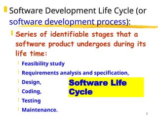
Software Life
Cycle
SoftwareDevelopment Life Cycle (or
software development process):
Series of identifiable stages that a
software product undergoes during its
life time:
Feasibility study
Requirements analysis and specification,
Design,
Coding,
Testing
Maintenance.
4.
4
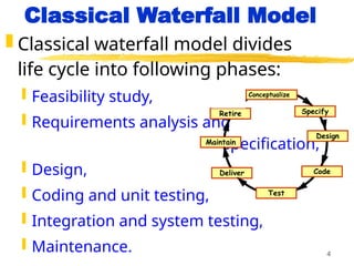
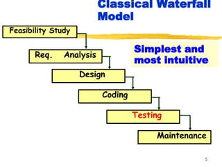
Classical Waterfall Model
Classical waterfall model divides
life cycle into following phases:
Feasibility study,
Requirements analysis and
specification,
Design,
Coding and unit testing,
Integration and system testing,
Maintenance.
Conceptualize
Specify
Design
Code
Test
Maintain
Retire
Deliver
7
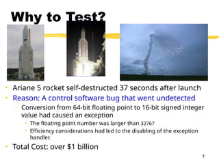
Why to Test?
•Ariane 5 rocket self-destructed 37 seconds after launch
• Reason: A control software bug that went undetected
– Conversion from 64-bit floating point to 16-bit signed integer
value had caused an exception
• The floating point number was larger than 32767
• Efficiency considerations had led to the disabling of the exception
handler.
• Total Cost: over $1 billion
8.
8
Organization of this
lecture
Important concepts in program
testing
Black-box testing:
equivalence partitioning
boundary value analysis
White-box testing
Debugging
Unit, Integration, and System testing
Summary
9.
9
How Do YouTest a
Program?
Input test data to the program.
Observe the output:
Check if the program behaved as
expected.
11
How Do YouTest a
Program?
If the program does not behave
as expected:
Note the conditions under which it
failed.
Later debug and correct.
12.
12
What’s So HardAbout
Testing ?
Consider int proc1(int x, int y)
Assuming a 64 bit computer
Input space = 2128
Assuming it takes 10secs to key-in an integer pair
It would take about a billion years to enter all
possible values!
Automatic testing has its own problems!
13.
13
Testing Facts
Consumeslargest effort among all
phases
Largest manpower among all other
development roles
Implies more job opportunities
About 50% development effort
But 10% of development time?
How?
14.
14
Testing Facts
Testingis getting more complex
and sophisticated every year.
Larger and more complex
programs
Newer programming paradigms
15.
15
Overview of Testing
Activities
Test Suite Design
Run test cases and observe
results to detect failures.
Debug to locate errors
Correct errors.
16.
16
Error, Faults, and
Failures
Afailure is a manifestation of
an error (also defect or bug).
Mere presence of an error may
not lead to a failure.
17.
17
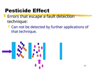
Pesticide Effect
Errorsthat escape a fault detection
technique:
Can not be detected by further applications of
that technique.
18.
18
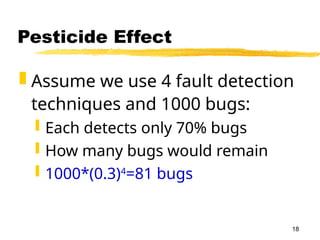
Pesticide Effect
Assumewe use 4 fault detection
techniques and 1000 bugs:
Each detects only 70% bugs
How many bugs would remain
1000*(0.3)4
=81 bugs
19.
19
Fault Model
Typesof faults possible in a
program.
Some types can be ruled out
Concurrency related-problems in a
sequential program
20.
20
Fault Model ofan OO
Program
OO Faults
Structural
Faults
Algorithmic
Faults
Procedural
Faults
Traceabilit
y Faults
OO
Faults
Incorrect
Result
Inadequate
Performanc
e
21.
21
Hardware Fault-Model
Simple:
Stuck-at 0
Stuck-at 1
Open circuit
Short circuit
Simple ways to test the presence of each
Hardware testing is fault-based testing
22.
22
Software Testing
Eachtest case typically tries to establish
correct working of some functionality
Executes (covers) some program elements
For restricted types of faults, fault-based
testing exists.
23.
23
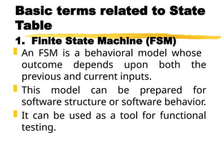
Test Cases andTest
Suites
Test a software using a set
of carefully designed test
cases:
The set of all test cases is
called the test suite
24.
24
Test Cases andTest
Suites
A test case is a triplet [I,S,O]
I is the data to be input to the
system,
S is the state of the system at
which the data will be input,
O is the expected output of the
system.
25.
25
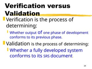
Verification versus
Validation
Verificationis the process of
determining:
Whether output of one phase of development
conforms to its previous phase.
Validation is the process of determining:
Whether a fully developed system
conforms to its SRS document.
27
Design of TestCases
Exhaustive testing of any non-
trivial system is impractical:
Input data domain is extremely large.
Design an optimal test suite:
Of reasonable size and
Uncovers as many errors as
possible.
28.
28
Design of TestCases
If test cases are selected randomly:
Many test cases would not contribute to the
significance of the test suite,
Would not detect errors not already being
detected by other test cases in the suite.
Number of test cases in a randomly selected
test suite:
Not an indication of effectiveness of testing.
29.
29
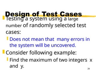
Design of TestCases
Testing a system using a large
number of randomly selected test
cases:
Does not mean that many errors in
the system will be uncovered.
Consider following example:
Find the maximum of two integers x
and y.
30.
30
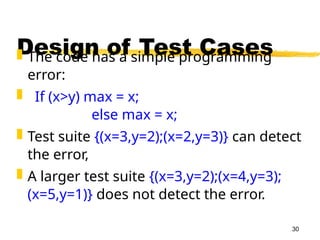
Design of TestCases
The code has a simple programming
error:
If (x>y) max = x;
else max = x;
Test suite {(x=3,y=2);(x=2,y=3)} can detect
the error,
A larger test suite {(x=3,y=2);(x=4,y=3);
(x=5,y=1)} does not detect the error.
31.
31
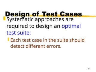
Design of TestCases
Systematic approaches are
required to design an optimal
test suite:
Each test case in the suite should
detect different errors.
32.
32
Design of Test
Cases
Thereare essentially three
main approaches to design
test cases:
Black-box approach
White-box (or glass-box)
approach
33.
33
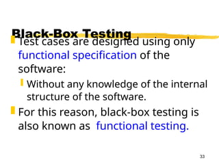
Black-Box Testing
Testcases are designed using only
functional specification of the
software:
Without any knowledge of the internal
structure of the software.
For this reason, black-box testing is
also known as functional testing.
34.
34
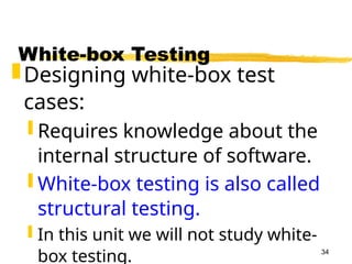
White-box Testing
Designing white-boxtest
cases:
Requires knowledge about the
internal structure of software.
White-box testing is also called
structural testing.
In this unit we will not study white-
box testing.
36
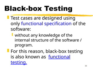
Black-box Testing
Testcases are designed using
only functional specification of the
software:
without any knowledge of the
internal structure of the software /
program.
For this reason, black-box testing
is also known as functional
testing.
37.
37
Black-box Testing
Thereare essentially two
main approaches to design
black box test cases:
Equivalence class partitioning
Boundary value analysis
38.
38
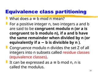
Equivalence class partitioning
What does a b mod n mean?
≡
For a positive integer n, two integers a and b
are said to be congruent modulo n (or a is
congruent to b modulo n), if a and b have
the same remainder when divided by n (or
equivalently if a b is divisible by n )
− .
Congruence modulo n divides the set Z of all
integers into n subsets called residue classes
(equivalence classes).
It can be expressed as a b mod n, n is
≡
called the modulus.
39.
39
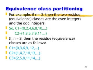
Equivalence class partitioning
For example, if n = 2, then the two residue
(equivalence) classes are the even integers
and the odd integers.
So, C1={0,2,4,6,8,10,…}
C2={1,3,5,7,9,11,…}
If, n = 3, then the residue (equivalence)
classes are as follows:
C1={0,3,6,9, 12,…}
C2={1,4,7,10,13,…}
C3={2,5,8,11,14,…}
40.
40
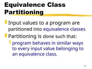
Equivalence Class
Partitioning
Inputvalues to a program are
partitioned into equivalence classes.
Partitioning is done such that:
program behaves in similar ways
to every input value belonging to
an equivalence class.
41.
41
Why define equivalence
classes?
Test the code with just one
representative value from
each equivalence class:
as good as testing using any
other values from the
equivalence classes.
42.
42
Equivalence Class
Partitioning
Howdo you determine the
equivalence classes?
examine the input data.
few general guidelines for
determining the equivalence
classes can be given
43.
43
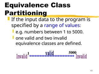
Equivalence Class
Partitioning
Ifthe input data to the program is
specified by a range of values:
e.g. numbers between 1 to 5000.
one valid and two invalid
equivalence classes are defined.
1 5000
44.
44
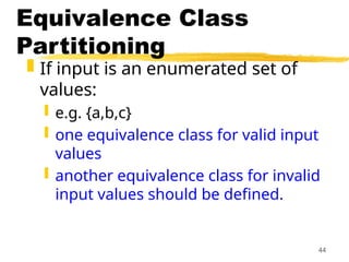
Equivalence Class
Partitioning
Ifinput is an enumerated set of
values:
e.g. {a,b,c}
one equivalence class for valid input
values
another equivalence class for invalid
input values should be defined.
45.
45
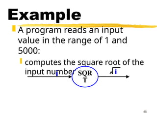
Example
A programreads an input
value in the range of 1 and
5000:
computes the square root of the
input number SQR
T
46.
46
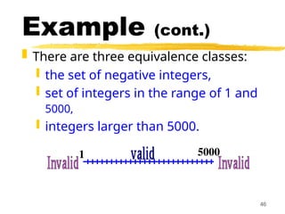
Example (cont.)
Thereare three equivalence classes:
the set of negative integers,
set of integers in the range of 1 and
5000,
integers larger than 5000.
1 5000
47.
47
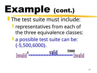
Example (cont.)
Thetest suite must include:
representatives from each of
the three equivalence classes:
a possible test suite can be:
{-5,500,6000}.
1 5000
48.
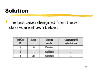
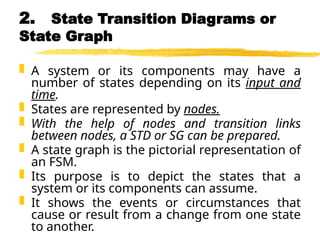
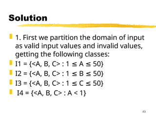
Example
A programreads three numbers, A, B,
and C, with a range [1, 50] and prints
the largest number. Design test cases
for this program using equivalence
class testing technique.
48
49.
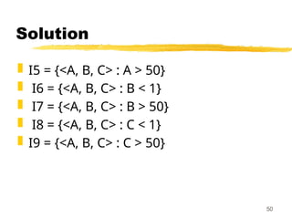
Solution
1. Firstwe partition the domain of input
as valid input values and invalid values,
getting the following classes:
I1 = {<A, B, C> : 1 A 50}
≤ ≤
I2 = {<A, B, C> : 1 B 50}
≤ ≤
I3 = {<A, B, C> : 1 C 50}
≤ ≤
I4 = {<A, B, C> : A < 1}
49
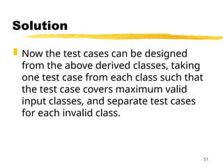
Solution
Now thetest cases can be designed
from the above derived classes, taking
one test case from each class such that
the test case covers maximum valid
input classes, and separate test cases
for each invalid class.
51
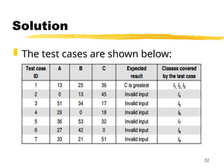
Solution
2. Wecan derive another set of
equivalence classes based on some
possibilities for three integers, A, B, and
C. These are given below:
I1 = {<A, B, C> : A > B, A > C}
I2 = {<A, B, C> : B > A, B > C}
I3 = {<A, B, C> : C > A, C > B}
53
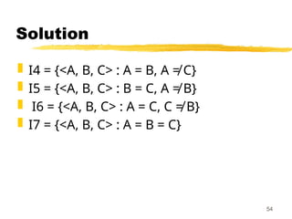
54.
Solution
I4 ={<A, B, C> : A = B, A ≠ C}
I5 = {<A, B, C> : B = C, A ≠ B}
I6 = {<A, B, C> : A = C, C ≠ B}
I7 = {<A, B, C> : A = B = C}
54
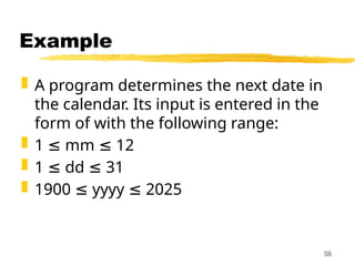
Example
A programdetermines the next date in
the calendar. Its input is entered in the
form of with the following range:
1 mm 12
≤ ≤
1 dd 31
≤ ≤
1900 yyyy 2025
≤ ≤
56
57.
Example
Its outputwould be the next date or an
error message ‘invalid date.’ Design test
cases using equivalence class
partitioning method.
57
58.
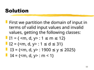
Solution
First wepartition the domain of input in
terms of valid input values and invalid
values, getting the following classes:
I1 = { <m, d, y> : 1 m 12}
≤ ≤
I2 = {<m, d, y> : 1 d 31}
≤ ≤
I3 = {<m, d, y> : 1900 y 2025}
≤ ≤
I4 = {<m, d, y> : m < 1}
58
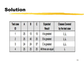
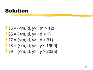
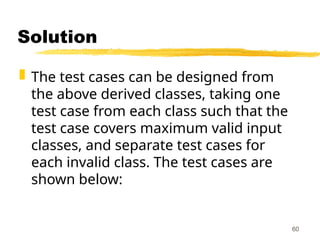
Solution
The testcases can be designed from
the above derived classes, taking one
test case from each class such that the
test case covers maximum valid input
classes, and separate test cases for
each invalid class. The test cases are
shown below:
60
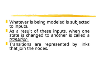
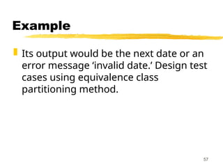
Example
A programtakes an angle as input
within the range [0, 360] and
determines in which quadrant the angle
lies. Design test cases using
equivalence class partitioning method.
62
63.
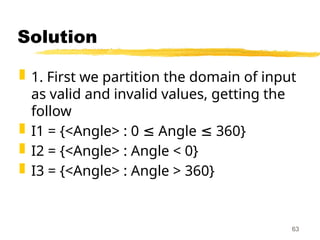
Solution
1. Firstwe partition the domain of input
as valid and invalid values, getting the
follow
I1 = {<Angle> : 0 Angle 360}
≤ ≤
I2 = {<Angle> : Angle < 0}
I3 = {<Angle> : Angle > 360}
63
Solution
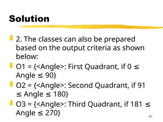
2. Theclasses can also be prepared
based on the output criteria as shown
below:
O1 = {<Angle>: First Quadrant, if 0 ≤
Angle 90}
≤
O2 = {<Angle>: Second Quadrant, if 91
Angle 180}
≤ ≤
O3 = {<Angle>: Third Quadrant, if 181 ≤
Angle 270}
≤ 65
66.
Solution
O4 ={<Angle>: Fourth Quadrant, if 271
Angle 360}
≤ ≤
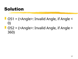
O5 = {<Angle>: Invalid Angle};
However, O5 is not sufficient to cover all
invalid conditions this way. Therefore, it
must be further divided into
equivalence classes as shown in next
slide:
66
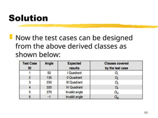
Solution
Now thetest cases can be designed
from the above derived classes as
shown below:
68
69.
69
Boundary Value
Analysis
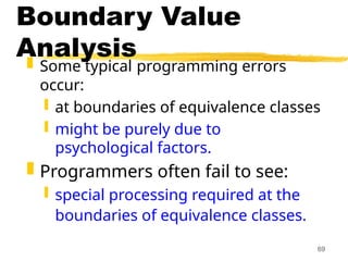
Sometypical programming errors
occur:
at boundaries of equivalence classes
might be purely due to
psychological factors.
Programmers often fail to see:
special processing required at the
boundaries of equivalence classes.
70.
70
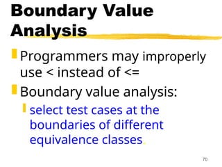
Boundary Value
Analysis
Programmersmay improperly
use < instead of <=
Boundary value analysis:
select test cases at the
boundaries of different
equivalence classes.
71.
71
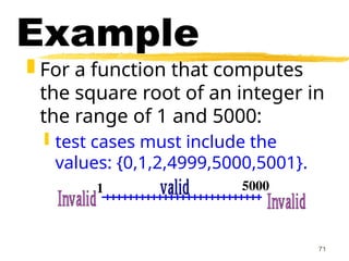
Example
For afunction that computes
the square root of an integer in
the range of 1 and 5000:
test cases must include the
values: {0,1,2,4999,5000,5001}.
1 5000
Ex:-1
Q. Checkif 2 Straight Lines Intersect and Print Their Point of
Intersection
Ans: y = mx + c
Straight lines are given in the form of (m1, c1) and (m2, c2)
Step:1
Identify the Equivalent class
Case 1: The lines are parallel i.e. m1 = m2
So points are (1, 2) and (1, 5)
Case 2: Coincident lines i.e. m1 = m2 and c1= c2
And points are (2, 3) and (2, 3)
75.
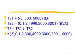
Ex:-1 Contd.
Case3: Lines intersecting at one point i.e.
The points may be (2, 5) and (3, 6).
So there are 3 equivalent classes.
There are no boundary values here.
So, Test Suite = {(1, 2),(1, 5),(2, 3),(2, 3),(2, 5),(3, 6)}
2
1 m
m
76.
Ex:-2
The ProgramSolves quadratic equations of the form
It will accept 3 floating point values as input and it will
gives the roots e.g. The input may be (7.7, 3.3 and 4.5).
Ans: Equivalent Classes
I. b2
=4ac inputs are: a= 2.0, b=4.0 and c=2.0
II. b2
>4ac inputs are a=2.0, b= 5.0 and c=2.0
III. b2
<4ac inputs are a=2.0, b= 3.0 and c=2.0
IV. Invalid Equation inputs are a=0, b= 0 and c=10.0
So, Test Suite = {(2.0,4.0,2.0),(2.0,5.0,2.0),(2.0,3.0,2.0),(0.0,0.0,10.0)}
c
bx
ax
2
77.
Ex:-3
Solves linearequations in upto 10 independent variables
e.g. 5x+6y+z=5
10x+2y+5z=20
…………
…………
78.
Example
Equivalent Classes
I.Valid
a. Many Solution (# var < #eqns)
b. No Solution (# var > #eqns)
c. Unique Solution (# var = #eqns)
II.Invalid
a. Too many Variables (# var > 10)
b. Invalid Equation (# var = 0)
79.
Ex:-3
Program Findspoints of intersection of 2 circles
Equivalent Classes
I. r1+r2< distance between(x1, y1) and (x2, y2) i.e. not intersecting
II. r1+r2= distance i.e. touching at 1 point
III.r1+r2> distance i.e. intersecting at 2 points
IV.Distance=0 and r1= r2 i.e. overlapping
V. Distance=0 and r1≠ r2
VI.Invalid circles
80.
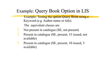
Example: Query BookOption in LIS
Example: Testing the option Query Book using a
Keyword (e.g. Author name or title).
The equivalent classes are
Not present in catalogue (SE, not present)
Present in catalogue (SE, present, 15 issued, not
available)
Present in catalogue (SE, present, 10 issued, 5
available)
81.
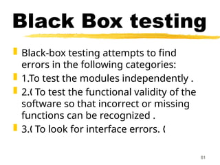
Black Box testing
Black-box testing attempts to find
errors in the following categories:
1.To test the modules independently .
2. To test the functional validity of the
„
software so that incorrect or missing
functions can be recognized .
3. To look for interface errors.
„ „
81
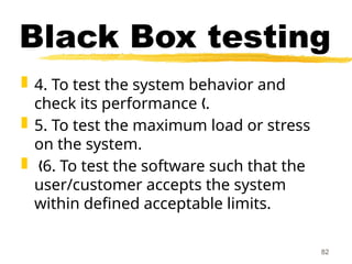
82.
4. Totest the system behavior and
check its performance .
„
5. To test the maximum load or stress
on the system.
6. To test the software such that the
„
user/customer accepts the system
within defined acceptable limits.
82
Black Box testing
83.
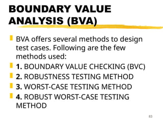
BOUNDARY VALUE
ANALYSIS (BVA)
BVA offers several methods to design
test cases. Following are the few
methods used:
1. BOUNDARY VALUE CHECKING (BVC)
2. ROBUSTNESS TESTING METHOD
3. WORST-CASE TESTING METHOD
4. ROBUST WORST-CASE TESTING
METHOD
83
84.
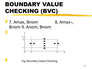
BOUNDARY VALUE
CHECKING (BVC)
In this method, the test cases are
designed by holding one variable at its
extreme value and other variables at
their nominal values in the input
domain.
The variable at its extreme value can be
selected at:
84
85.
BOUNDARY VALUE
CHECKING (BVC)
(a) Minimum value (Min)
(b) Value just above the minimum value
(Min+ )
(c) Maximum value (Max)
(d) Value just below the maximum value
(Max )
−
85
86.
BOUNDARY VALUE
CHECKING (BVC)
Let us take the example of two
variables, A and B.
If we consider all the above
combinations with nominal values, then
following test cases (see Fig. 1) can be
designed:
1. Anom, Bmin 2. Anom, Bmin+
3. Anom, Bmax 4. Anom, Bmax–
5. Amin, Bnom 6. Amin+, Bnom
86
BOUNDARY VALUE
CHECKING (BVC)
It can be generalized that for n
variables in a module, 4n + 1 test cases
can be designed with boundary value
checking method.
88
89.
ROBUSTNESS TESTING
METHOD
Theidea of BVC can be extended such
that boundary values are exceeded as: „
1. A value just greater than the
Maximum value (Max+)
2. A value just less than Minimum value
„
(Min )
−
89
90.
ROBUSTNESS TESTING
METHOD
Whentest cases are designed
considering the above points in
addition to BVC, it is called robustness
testing.
Let us take the previous example again.
Add the following test cases to the list
of 9 test cases designed in BVC:
10. Amax+, Bnom 11. Amin–, Bnom
90
91.
ROBUSTNESS TESTING
METHOD
12.Anom, Bmax+ 13. Anom, Bmin–
It can be generalized that for n input
variables in a module, 6n + 1 test cases
can be designed with robustness
testing.
91
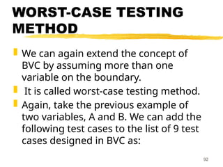
92.
WORST-CASE TESTING
METHOD
Wecan again extend the concept of
BVC by assuming more than one
variable on the boundary.
It is called worst-case testing method.
Again, take the previous example of
two variables, A and B. We can add the
following test cases to the list of 9 test
cases designed in BVC as:
92
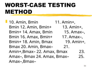
WORST-CASE TESTING
METHOD
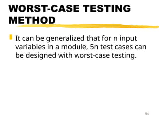
Itcan be generalized that for n input
variables in a module, 5n test cases can
be designed with worst-case testing.
94
95.
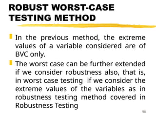
ROBUST WORST-CASE
TESTING METHOD
In the previous method, the extreme
values of a variable considered are of
BVC only.
The worst case can be further extended
if we consider robustness also, that is,
in worst case testing if we consider the
extreme values of the variables as in
robustness testing method covered in
Robustness Testing
95
96.
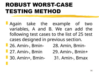
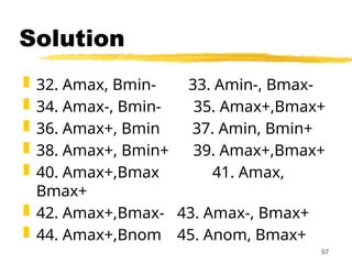
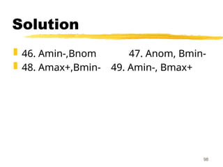
ROBUST WORST-CASE
TESTING METHOD
Again take the example of two
variables, A and B. We can add the
following test cases to the list of 25 test
cases designed in previous section.
26. Amin-, Bmin- 28. Amin, Bmin-
27. Amin-, Bmin 29. Amin-, Bmin+
30. Amin+, Bmin- 31. Amin-, Bmax
96
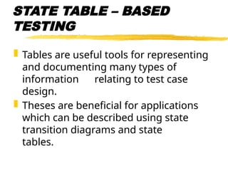
STATE TABLE –BASED
TESTING
Tables are useful tools for representing
and documenting many types of
information relating to test case
design.
Theses are beneficial for applications
which can be described using state
transition diagrams and state
tables.
100.
Basic terms relatedto State
Table
1. Finite State Machine (FSM)
An FSM is a behavioral model whose
outcome depends upon both the
previous and current inputs.
This model can be prepared for
software structure or software behavior.
It can be used as a tool for functional
testing.
101.
2. State TransitionDiagrams or
State Graph
A system or its components may have a
number of states depending on its input and
time.
States are represented by nodes.
With the help of nodes and transition links
between nodes, a STD or SG can be prepared.
A state graph is the pictorial representation of
an FSM.
Its purpose is to depict the states that a
system or its components can assume.
It shows the events or circumstances that
cause or result from a change from one state
to another.
102.
Whatever isbeing modeled is subjected
to inputs.
As a result of these inputs, when one
state is changed to another is called a
transition.
Transitions are represented by links
that join the nodes.
103.
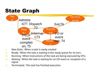
For example, atask in an O. S. can have
its following states:
i. New State : When a task is newly created
ii. Ready : When the task is waiting in the
ready queue for its turn.
iii. Running : When Instructions of the task are
being executed by CPU.
iv. Waiting : When the task is waiting for an I/O
event or reception of a signal
v. Terminated : The task has finished
execution.
104.
State Graph
i. NewState : When a task is newly created
ii. Ready : When the task is waiting in the ready queue for its turn.
iii. Running : When Instructions of the task are being executed by CPU.
iv. Waiting : When the task is waiting for an I/O event or reception of a
signal
v. Terminated : The task has finished execution.
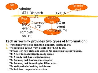
Ne
w
Rea
dy
Runni
ng
Termin
ated
Waitin
g
Admitte
d,T1 Dispatch
,T2
Exit,T6
Interrup
t,T3
I/O or
event
completi
on, T5
I/O or
event
wait, T4
105.
Each arrow linkprovides two types of Information :
1. Transition events like admitted, dispatch, interrupt, etc.
2. The resulting output from a state like T1, T2, T3 etc.
T0=Task is in new state and waiting for admission to ready queue.
T1= A new task admitted to ready queue
T2= A ready task has started running
T3= Running task has been interrupted
T4= Running task is waiting for I/O or event
T5= Wait period of waiting task is over
T6= Task has completed execution
Ne
w
Rea
dy
Runni
ng
Termin
ated
Waitin
g
Admitte
d,T1 Dispatch
,T2
Exit,T6
Interrup
t,T3
I/O or
event
completi
on, T5
I/O or
event
wait, T4
106.
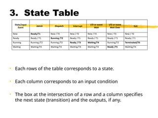
3. State Table
•Each rows of the table corresponds to a state.
• Each column corresponds to an input condition
• The box at the intersection of a row and a column specifies
the next state (transition) and the outputs, if any.
State/input
Event
Admit Dispatch Interrupt
I/O or event
Wait
I/O or event
Wait Over
Exit
New Ready/T1 New / T0 New / T0 New / T0 New / T0 New / T0
Ready Ready / T1 Running /T2 Ready / T1 Ready / T1 Ready / T1 Ready / T1
Running Running /T2 Running /T2 Ready / T3 Waiting/T4 Running/T2 Terminated/T6
Waiting Waiting/T4 Waiting/T4 Waiting/T4 Waiting/T4 Ready /T5 Waiting/T4
107.
4. State Table-BasedTesting
After reviewing the basics, we can start
functional testing with state tables.
Steps:
1. Identify the states
The number of states in a state graph is
the number of states we choose to
recognize or model.
108.
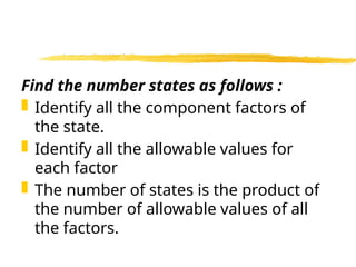
Find the numberstates as follows :
Identify all the component factors of
the state.
Identify all the allowable values for
each factor
The number of states is the product of
the number of allowable values of all
the factors.
109.
2. Prepare statetransition diagram
after understanding transitions
between states
After having all the states, identify the
inputs on each state and transitions
between states and prepare the state
graph.
Every input state combination must
have a specified transition.
110.
3. Convert thestate graph into the
state table as discussed earlier
4. Analyze the state table for its
completeness.
111.
5. Create thecorresponding test cases from the
state table
• Test cases are produced in a tabular form known as the test case.
• Test cases ID : a unique identifier for each test case
• Test Source : a trace back to the corresponding cell in the state table.
• Current state : the initial condition to run the test
• Event : the input triggered by the user
• Output : the current value returned
• Next State : the new state achieved
Test case ID Test Source
Input Expected results
Current State Event Output Next state
TC1 Cell 1 New Admit T1 Ready
TC2 Cell 2 New Dispatch T0 New
TC3 Cell 3 New Interrupt T0 New
TC4 Cell 4 New I/O wait T0 New
TC5 Cell 5 New I/O wait over T0 New
TC6 Cell 6 New Exit T0 New
TC7 Cell 7 Ready Admit T1 Ready
TC8 Cell 8 Ready Dispatch T2 Running
TC9 Cell 9 Ready Interrupt T1 Ready
TC10 Cell 10 Ready I/O wait T1 Ready
TC11 Cell 11 Ready I/O wait over T1 Ready
TC12 Cell 12 Ready Exit T1 Ready
TC13 Cell 13 Running Admit T2 Running
TC14 Cell 14 Running Dispatch T2 Running
TC15 Cell 15 Running Interrupt T3 Ready
TC16 Cell 16 Running I/O wait T4 Waiting
TC17 Cell 17 Running I/O wait over T2 Running
TC18 Cell 18 Running Exit T6 Terminated
TC19 Cell 19 Waiting Admit T4 Waiting
TC20 Cell 20 Waiting Dispatch T4 Waiting
TC21 Cell 21 Waiting Interrupt T4 Waiting
TC22 Cell 22 Waiting I/O wait T4 Waiting
TC23 Cell 23 Waiting I/O wait over T5 Ready
TC24 Cell 24 Waiting Exit T4 Waiting
112.
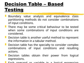
Decision Table –Based
Testing
Boundary value analysis and equivalence class
partitioning methods do not consider combinations
of input conditions.
There may be some critical behaviour to be tested
when some combinations of input conditions are
considered.
Decision table is another useful method to represent
the information in a tabular method.
Decision table has the specialty to consider complex
combinations of input conditions and resulting
actions.
Decision tables obtain their power from logical
expressions.
113.
Formation of Decision
Table
Conditionstub It is a list a list of input conditions for which the complex combination is made.
Action stub It is a list of resulting action which will be performed if a combination of input condition is
satisfied.
Condition entry
• It is a specific entry in the table corresponding to input conditions mentioned in the condition stub.
• When the condition entry takes only two values – TRUE or FALSE then it is called Limited Entry Decision
Table.
• When the condition entry takes several values , then it is called Extended Entry Decision Table.
Action entry It is the entry in the table for the resulting action to be performed
• List all actions that can be associated with a specific procedure.
• List all conditions during execution of the procedure.
• Associate specific sets of conditions with specific actions, eliminating impossible combinations and
conditions; alternatively, develop every possible permutation of conditions.
• Define rules by indicating what action occurs for a set of conditions.
Condition
Stub
Rule 1 Rule 2 Rule 3 Rule 4 ...
C1
C2
C3
True
False
True
True
True
True
False
False
True
I
True
I
Action Stub
A1
A2
A3
X X
X
X
114.
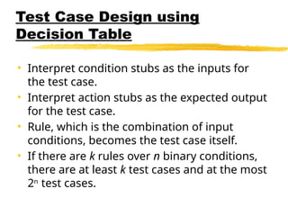
Test Case Designusing
Decision Table
• Interpret condition stubs as the inputs for
the test case.
• Interpret action stubs as the expected output
for the test case.
• Rule, which is the combination of input
conditions, becomes the test case itself.
• If there are k rules over n binary conditions,
there are at least k test cases and at the most
2n
test cases.
115.
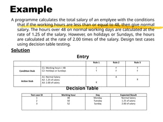
Example
A programme calculatesthe total salary of an emplyee with the conditions
that if the working hours are less than or equal to 48, then give normal
salary. The hours over 48 on normal working days are calculated at the
rate of 1.25 of the salary. However, on holidays or Sundays, the hours
are calculated at the rate of 2.00 times of the salary. Design test cases
using decision table testing.
Solution
Entry
Decision Table
Rule 1 Rule 2 Rule 3
Condition Stub
C1: Working hours > 48
C2: Holidays or Sundays
I
T
F
F
T
F
Action Stub
A1: Normal Salary
A2: 1.25 of salary
A3: 2.00 of salary X
X
X
Test case ID Working hour Day Expected Result
1
2
3
48
50
52
Monday
Tuesday
Sunday
Normal Salary
1.25 of salary
2.00 of salary
116.
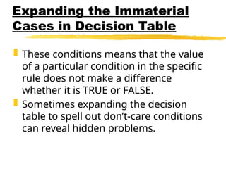
Expanding the Immaterial
Casesin Decision Table
These conditions means that the value
of a particular condition in the specific
rule does not make a difference
whether it is TRUE or FALSE.
Sometimes expanding the decision
table to spell out don’t-care conditions
can reveal hidden problems.
117.
Example
Entry (Decision table)
Theimmaterial test case in rule 1 of the
above table can be expanded by taking
both T and F values of C1.
Rule 1 Rule 2 Rule 3
Condition Stub
C1: Working hours > 48
C2: Holidays or Sundays
I
T
F
F
T
F
Action Stub
A1: Normal Salary
A2: 1.25 of salary
A3: 2.00 of salary X
X
X
118.
Entry (Expanded decision
table)
Entry(Expanded decision table)
Rule 1-1 Rule 1-2 Rule 2 Rule 3
Condition Stub
C1: Working hours > 48
C2: Holidays or Sundays
F
T
T
T
F
F
T
F
Action Stub
A1: Normal Salary
A2: 1.25 of salary
A3: 2.00 of salary X X
X
X
Test case ID Working hour Day Expected Result
1
2
3
4
48
50
52
30
Monday
Tuesday
Sunday
Sunday
Normal Salary
1.25 of salary
2.00 of salary
2.00 of salary
119.
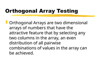
Orthogonal Arraysare two dimensional
arrays of numbers that have the
attractive feature that by selecting any
two columns in the array, an even
distribution of all pairwise
combinations of values in the array can
be achieved.
Orthogonal Array Testing
120.
In thefollowing table , after selecting
first two columns, we get four ordered
pairs namely (0,0), (1,1), (0,1) and (1,0).
These pairs form all the possible
ordered pairs of two-element set and
each ordered pair appears exactly once.
Example
121.
We obtain samevalues when selecting second and third or first
and third column combination. An array exhibiting this feature
is known as orthogonal array.
Example
122.
Orthogonal arrayscan be used in
software testing for pairwise
interactions.
It provides uniformly distributed
coverage for all variable pairwise
combinations.
It is commonly used for integration
testing like object oriented systems,
where multiple subclasses can be
Orthogonal Array Testing
123.
It isblack-box testing technique.
OATS is used when the input to the system to
be tested are low but if exhaustive testing is
used then it is not possible to test completely
every input of the system.
100% OATS implies 100% pairwise testing.
OATS can be used for testing combinations of
configurable options like a webpage that
allows the other user to select:
Orthogonal Array Testing
124.
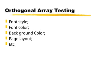
Font style;
Font color;
Back ground Color;
Page layout;
Etc.
Orthogonal Array Testing
125.
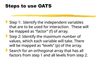
Step 1:Identify the independent variables
that are to be used for interaction. These will
be mapped as “factor” (f) of array.
Step 2: Identify the maximum number of
values, which each variable will take. There
will be mapped as “levels” (p) of the array.
Search for an orthogonal array that has all
factors from step 1 and all levels from step 2.
Steps to use OATS
126.
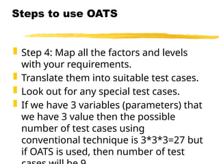
Step 4:Map all the factors and levels
with your requirements.
Translate them into suitable test cases.
Look out for any special test cases.
If we have 3 variables (parameters) that
we have 3 value then the possible
number of test cases using
conventional technique is 3*3*3=27 but
if OATS is used, then number of test
Steps to use OATS
127.
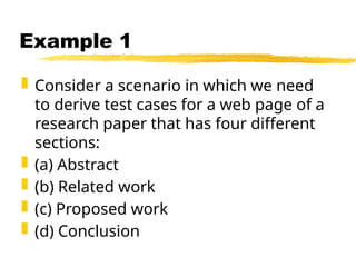
Consider ascenario in which we need
to derive test cases for a web page of a
research paper that has four different
sections:
(a) Abstract
(b) Related work
(c) Proposed work
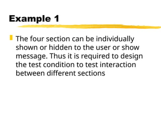
(d) Conclusion
Example 1
128.
The foursection can be individually
shown or hidden to the user or show
message. Thus it is required to design
the test condition to test interaction
between different sections
Example 1
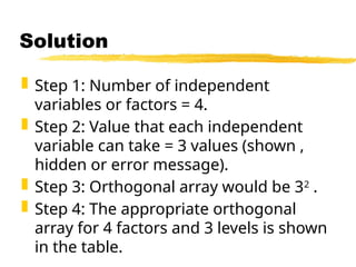
129.
Step 1:Number of independent
variables or factors = 4.
Step 2: Value that each independent
variable can take = 3 values (shown ,
hidden or error message).
Step 3: Orthogonal array would be 32
.
Step 4: The appropriate orthogonal
array for 4 factors and 3 levels is shown
in the table.
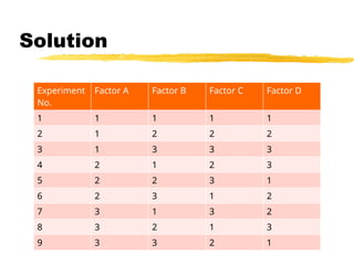
Solution
Step 5:Now, map the table with our
requirements.
1 will represent “Shown” value.
2 will represent “Hidden” value.
3 will represent “Error Message” value.
Factor A will represent “Abstract” section.
Factor B will represent “Related Work”
section.
Factor C will represent “Proposed Work”
section.
Solution
132.
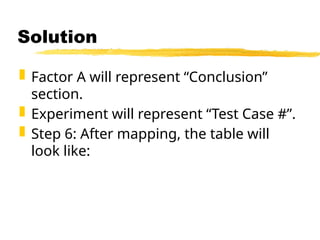
Factor Awill represent “Conclusion”
section.
Experiment will represent “Test Case #”.
Step 6: After mapping, the table will
look like:
Solution
133.
Test Case AbstractRelated Work Proposed
work
Conclusion
Test Case 1 Shown Shown Shown Shown
Test Case 2 Shown Hidden Hidden Hidden
Test Case 3 Shown Error
Message
Error
Message
Error
Message
Test Case 4 Hidden Shown Hidden Error
Message
Test Case 5 Hidden Hidden Error
Message
Shown
Test Case 6 Hidden Error
Message
Shown Hidden
Test Case 7 Error Shown Error Hidden
Solution
134.
134
Debugging
Once errorsare identified:
it is necessary identify the precise
location of the errors and to fix
them.
Each debugging approach has its
own advantages and
disadvantages:
each is useful in appropriate
circumstances.
135.
135
Brute-force method
Thisis the most common method
of debugging:
least efficient method.
program is loaded with print
statements
print the intermediate values
hope that some of printed values
will help identify the error.
136.
136
Symbolic Debugger
Bruteforce approach becomes
more systematic:
with the use of a symbolic
debugger,
symbolic debuggers get their name
for historical reasons
early debuggers let you only see
values from a program dump:
determine which variable it corresponds
to.
137.
137
Symbolic Debugger
Usinga symbolic debugger:
values of different variables can be
easily checked and modified
single stepping to execute one
instruction at a time
break points and watch points can
be set to test the values of variables.
138.
138
Backtracking
This isa fairly common
approach.
Beginning at the statement where
an error symptom has been
observed:
source code is traced backwards
until the error is discovered.
140
Backtracking
Unfortunately, asthe number of
source lines to be traced back
increases,
the number of potential backward
paths increases
becomes unmanageably large for
complex programs.
141.
141
Cause-elimination
method
Determine alist of causes:
which could possibly have
contributed to the error symptom.
tests are conducted to eliminate
each.
A related technique of identifying
error by examining error
symptoms:
software fault tree analysis.
142.
142
Program Slicing
Thistechnique is similar to back
tracking.
However, the search space is reduced
by defining slices.
A slice is defined for a particular
variable at a particular statement:
set of source lines preceding this
statement which can influence the value
of the variable.
144
Debugging
Guidelines
Debugging usuallyrequires a thorough
understanding of the program design.
Debugging may sometimes require full
redesign of the system.
A common mistake novice programmers
often make:
not fixing the error but the error
symptoms.
145.
145
Debugging
Guidelines
Be awareof the possibility:
an error correction may introduce
new errors.
After every round of error-fixing:
regression testing must be
carried out.
146.
146
Program Analysis
Tools
Anautomated tool:
takes program source code as input
produces reports regarding several
important characteristics of the
program,
such as size, complexity, adequacy
of commenting, adherence to
programming standards, etc.
147.
147
Program Analysis
Tools
Someprogram analysis tools:
produce reports regarding the
adequacy of the test cases.
There are essentially two categories
of program analysis tools:
Static analysis tools
Dynamic analysis tools
148.
148
Static Analysis
Tools
Staticanalysis tools:
assess properties of a
program without executing it.
Analyze the source code
provide analytical conclusions.
149.
149
Static Analysis
Tools
Whethercoding standards have been
adhered to?
Commenting is adequate?
Programming errors such as:
uninitialized variables
mismatch between actual and formal
parameters.
Variables declared but never used, etc.
150.
150
Static Analysis
Tools
Codewalk through and
inspection can also be
considered as static analysis
methods:
however, the term static program
analysis is generally used for
automated analysis tools.
151.
151
Dynamic Analysis
Tools
Dynamicprogram analysis
tools require the program
to be executed:
its behavior recorded.
Produce reports such as
adequacy of test cases.
152.
152
Testing
The aimof testing is to identify
all defects in a software product.
However, in practice even after
thorough testing:
one cannot guarantee that the
software is error-free.
153.
153
Testing
The inputdata domain of
most software products is
very large:
it is not practical to test the
software exhaustively with
each input data value.
154.
154
Testing
Testing doeshowever expose
many errors:
testing provides a practical way
of reducing defects in a system
increases the users' confidence
in a developed system.
155.
155
Testing
Testing isan important
development phase:
requires the maximum effort
among all development phases.
In a typical development
organization:
maximum number of software engineers
can be found to be engaged in testing
activities.
156.
156
Testing
Many engineershave the
wrong impression:
testing is a secondary activity
it is intellectually not as
stimulating as the other
development activities, etc.
157.
157
Testing
Testing asoftware product is in
fact:
as much challenging as initial
development activities such as
specification, design, and
coding.
Also, testing involves a lot of
creative thinking.
159
Unit testing
Duringunit testing,
modules are tested in
isolation:
If all modules were to be tested
together:
it may not be easy to
determine which module has
the error.
160.
160
Unit testing
Unit testingreduces
debugging effort several
folds.
Programmers carry out unit
testing immediately after
they complete the coding of
a module.
161.
161
Integration testing
Afterdifferent modules of a
system have been coded and
unit tested:
modules are integrated in steps
according to an integration plan
partially integrated system is
tested at each integration step.
165
Big bang Integration
Testing
Big bang approach is the
simplest integration testing
approach:
all the modules are simply put
together and tested.
this technique is used only for
very small systems.
166.
166
Big bang Integration
Testing
Main problems with this
approach:
if an error is found:
it is very difficult to localize the error
the error may potentially belong to any
of the modules being integrated.
debugging errors found during big
bang integration testing are very
expensive to fix.
167.
167
Bottom-up Integration
Testing
Integrateand test the bottom
level modules first.
A disadvantage of bottom-up
testing:
when the system is made up of a
large number of small subsystems.
This extreme case corresponds to
the big bang approach.
168.
168
Top-down integration
testing
Top-downintegration testing starts with
the main routine:
and one or two subordinate routines in the
system.
After the top-level 'skeleton’ has been
tested:
immediate subordinate modules of the
'skeleton’ are combined with it and tested.
169.
169
Mixed integration
testing
Mixed(or sandwiched)
integration testing:
uses both top-down and
bottom-up testing approaches.
Most common approach
170.
170
Integration
Testing
In top-downapproach:
testing waits till all top-level
modules are coded and unit
tested.
In bottom-up approach:
testing can start only after
bottom level modules are ready.
171.
171
System Testing
Thereare three main kinds
of system testing:
Alpha Testing
Beta Testing
Acceptance Testing
174
Acceptance Testing
Systemtesting performed by
the customer himself:
to determine whether the
system should be accepted or
rejected.
175.
175
Stress Testing
Stresstesting (aka endurance
testing):
impose abnormal input to stress the
capabilities of the software.
Input data volume, input data rate,
processing time, utilization of
memory, etc. are tested beyond the
designed capacity.
176.
176
How many errorsare
still remaining?
Seed the code with some known
errors:
artificial errors are introduced into
the program.
Check how many of the seeded
errors are detected during
testing.
177.
177
Error Seeding
Let:
N be the total number of errors in
the system
n of these errors be found by
testing.
S be the total number of seeded
errors,
s of the seeded errors be found
during testing.
179
Example
100 errorswere introduced.
90 of these errors were found
during testing
50 other errors were also found.
Remaining errors=
50 (100-90)/90 = 6
180.
180
Error Seeding
Thekind of seeded errors should
match closely with existing errors:
However, it is difficult to predict the
types of errors that exist.
Categories of remaining errors:
can be estimated by analyzing
historical data from similar projects.
181.
181
Summary
Exhaustive testingof almost
any non-trivial system is
impractical.
we need to design an optimal
test suite that would expose as
many errors as possible.
182.
182
Summary
If weselect test cases randomly:
many of the test cases may not
add to the significance of the test
suite.
There are two approaches to
testing:
black-box testing
white-box testing.
183.
183
Summary
Black boxtesting is also known as
functional testing.
Designing black box test cases:
requires understanding only SRS document
does not require any knowledge about
design and code.
Designing white box testing requires
knowledge about design and code.
184.
184
Summary
We discussedblack-box test
case design strategies:
equivalence partitioning
boundary value analysis
We discussed some important
issues in integration and
system testing.
Editor's Notes
#12 (But, can think about doing this many tests today)

![24
Test Cases and Test
Suites
A test case is a triplet [I,S,O]
I is the data to be input to the
system,
S is the state of the system at
which the data will be input,
O is the expected output of the
system.](https://image.slidesharecdn.com/blackboxtextingtechniques-251017162817-f5c7b99b/85/Mastering-Black-Box-Testing-Methods-Design-Techniques-and-Examples-24-320.jpg)
![Example
A program reads three numbers, A, B,
and C, with a range [1, 50] and prints
the largest number. Design test cases
for this program using equivalence
class testing technique.
48](https://image.slidesharecdn.com/blackboxtextingtechniques-251017162817-f5c7b99b/85/Mastering-Black-Box-Testing-Methods-Design-Techniques-and-Examples-48-320.jpg)
![Example
A program takes an angle as input
within the range [0, 360] and
determines in which quadrant the angle
lies. Design test cases using
equivalence class partitioning method.
62](https://image.slidesharecdn.com/blackboxtextingtechniques-251017162817-f5c7b99b/85/Mastering-Black-Box-Testing-Methods-Design-Techniques-and-Examples-62-320.jpg)