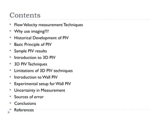
The document presents an extensive overview of various flow velocity measurement techniques, with a focus on three-dimensional particle image velocimetry (3D PIV) and wall PIV. It discusses the principles, historical development, techniques, limitations, experimental setup, and measurement uncertainties of PIV methods. Conclusions highlight the capabilities and accuracy of these techniques in measuring flow fields near walls with specific uncertainties addressed.

1. Three Dimensional, wall
Particle Image Velocimetry
Pawan Kumar
16ME62R07

2. Contents
 FlowVelocity measurement Techniques
 Why use imaging???
 Historical Development of PIV
 Basic Principle of PIV
 Sample PIV results
 Introduction to 3D PIV
 3D PIV Techniques
 Limitations of 3D PIV techniques
 Introduction toWall PIV
 Experimental setup forWall PIV
 Uncertainty in Measurement
 Sources of error
 Conclusions
 References

3. Flow Velocity Measurement Techniques
Source: MIT Open Courseware [2]

4. Intrusive Techniques
A Pitot Static Tube
Source: NPTEL Mechanical [3]
Hot wire thermal Anemometer
A,B and n are calibration constants

5. Non Intrusive Techniques
 Frequency Shift Based
Methods
Based on the Doppler
phenomenon, namely the
shift of the frequency of
waves scattered by moving
particles.
(a)Laser DopplerVelocimetry
(b)Planar DopplerVelocimetry
 Particle ImageVelocimetry
Technique
An optical method of flow
visualization

6. Laser Doppler Velocimetry
Doppler shift (fD) =V*(cosine(φs)-cosine(φi))/λ
Source: NPTEL Mechanical [3]

7. Planar Doppler Velocimetry
 Uses the principle of Doppler shift upon scattering.
 The Doppler shifted scattered light is split into two
paths using a beam-splitter and imaged onto the
camera(s) (as it passes through an iodine cell).
 For scattering by relatively large particles, this
absorption is a function of particle velocity alone.

8. Particle Image Velocimetry Technique
 Particle displacement method: to measure the
displacements of the tracer particles seeded in the flow in
a fixed time interval
Source: MIT Open Courseware [2]

9. Why Use Imaging?
Conventional Methods
(HWA, LDV) Particle ImageVelocimetry
 Single point measurement
 Traversing of flow domain
 Time consuming
 Only turbulence statistics
(e.g. the mean velocity,
turbulence intensity and
Reynolds stress, does not
represent the actual flow
structure)
 Whole field method
 Non-Intrusive (seeding)
 Instantaneous flow field

10. Historical Development
 Quantitative velocity data from particle streak photographs (1930)
 PIV was born as Laser SpeckleVelocimetry
Source: Particle Image Velocimetry
By Ronald J. Adrian, Jerry Westerweel [4]
Particle Streak

11. Historical Development
 Laser Speckle Velocimetry; Young’s fringes analysis
(Dudderar & Simpkins 1977)
 The specific characteristic of scattered laser light that
causes the phenomenon called “speckle” was used to
allow the measurement of the displacements of the
surface of samples subjected to strains.
Source: Wikipedia[10]

12. Basic Principle of PIV
 Based upon the measurement of the velocity of tracer
particles in the fluid.
 A plane of the flow under investigation is illuminated
using a laser
 Tracer particles are therefore made visible and images of
the illuminated particles will be recorded
 The instantaneous velocity of a fluid is measured through
the determination of the displacements of tracer particles
illuminated by a sheet of light

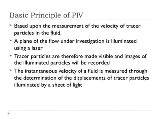
13. Basic Principle of PIV
 The actual measurement is consequently performed in
two successive steps:
(a)Recording of images
(b)Processing of the images to determine the tracer
displacement.
Source: MIT Open Courseware [2]

14. Basic Principle of PIV
Source: MIT Open Courseware [2]

15. PIV Results
Source: MIT Open Courseware [2]

16. PIV Results
Source: MIT Open Courseware [2]

17. PIV Results
Source: MIT Open Courseware [2]

18. Introduction to 3D-PIV
 In general, velocity components towards or away from the
camera are not calculated.
 Absence of z-component of velocity may also lead to an error
in x,y components due to parallax.
 Other PIV techniques are used for obtaining the third
component of velocity field, such as:-
(a)Scanning PIV
(b)Defocusing PIV
(c)Holographic PIV
(d)Tomographic PIV
(e)3D -PTV

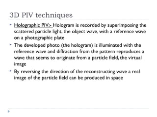
19. 3D PIV techniques
 Scanning PIV:- One or more cameras observe the
measurement volume as a laser sheet is scanned across it.
Source: Lawson M. John, Dawson R. James (2014) [5]

20. 3D PIV techniques
 Defocusing PIV:- A point in space off-axis from an
aperture will have an image that experiences a lateral
offset as the point moves along the axis of the optical
system.
Source: Francisco Pereira and Morteza Gharib [6]

21. 3D PIV techniques
 Holographic PIV:- Hologram is recorded by superimposing the
scattered particle light, the object wave, with a reference wave
on a photographic plate
 The developed photo (the hologram) is illuminated with the
reference wave and diffraction from the pattern reproduces a
wave that seems to originate from a particle field, the virtual
image
 By reversing the direction of the reconstructing wave a real
image of the particle field can be produced in space

22. 3D PIV techniques
Source: Hinsch K.D. (2002) [7]

23. 3D PIV techniques
 Tomographic PIV:- Tracer particles within the measurement
volume are illuminated by a pulsed light source and the
scattered light pattern is recorded simultaneously from several
viewing directions using CCD cameras.
Source: G.E. Elsinga, F. Scarano, B. Wieneke, B.W. etal (2005) [8]

24. 3D PIV techniques
 3D-PTV:- The particles located in a seeded volume are
imaged by three or four synchronized CCD cameras
arranged convergently.
 The cameras and the illumination must be mounted on a
platform moving approximately with the mean velocity of
the flow
Source: Marko Virant and Themistocles Dracos (1997) [9]

25. Limitations
 Scanning PIV
 Holographic PIV
 Not suitable for thin (few
hundred micrometers) near
wall regions as the
characteristic time scale of
the flow is small compared
to scanning time.
 Complicated and requires
high resolution CCD
cameras.

26. Limitations
 3D PTV and DDPIV
 Tomographic PIV
 Ambiguities in particles
positions resulting from
reconstruction approach.
 Higher processing time as
compared to DDPIV and
Wall PIV

27. Introduction to Wall PIV
 Tracer particles are seeded in a dyed fluid in a transparent
flow model.
 Intensity of scattered light after absorption through the dye is
given by Beer-Lambert Law
I-intensity of scattered light
I0-intensity of source
ε-absorbance coefficient of dye
R-penetration depth

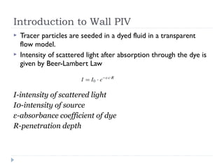
28. Introduction to Wall PIV
 Particles near the wall appear brighter than particles farther
away from the wall.This, together with the x- and y-position of
the particle in the image, allows the particle’s three-
dimensional position to be obtained
Source: Berthe Andre´, Kondermann Daniel
etal (2009)[1]

29. Experimental Setup
 Cameras:-CCD (250 fps) and CMOS (2000 fps)
 Molecular dye:-Patent blueV
 Tracer Particles:-silver-coated hollow ceramic spheres (73 to
75 μm)
 Illumination source:-3 W Luxeon LED (λ=617 nm and 627 nm)

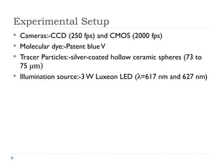
30. Experimental Setup
Source: Berthe Andre´, Kondermann Daniel
etal (2009)[1]

31. Experimental Setup
Transmission of patent blue V and relative spectra of the used
LEDs. Crosses represent the red wavelength, circles the orange
wavelength
Source: Berthe Andre´,
Kondermann Daniel etal (2009)
[1]

32. Uncertainty in measurement
 Particle depth is calculated as
 Uncertainty in the result can be calculated as

33. Uncertainty in measurement
Particle Position Relative uncertainty
 almost touching the wall
 At a distance of 38 μm
from the wall
 At a distance of 150 μm
from the wall
 10 %
 5 %
 2 %
Uncertainty in the particle size has the major impact on
relative uncertainty, followed by the uncertainty in the
intensity of illumination source. All others account for
less than 0.5%.

34. Error
 The accuracy depends upon the ability of the particle to
follow the fluid path.
 The particle motion can be analyzed by Basset-
Boussinesq-Oseen equation
 mp, v(t) and a are the particle mass, velocity, and radius
 ρ,mf, μ and ν are the density, displaced-mass, dynamic
viscosity, and kinematic viscosity of the fluid

35. Conclusions
 Capable of measurement of flow fields near vaulted
and/or deformable walls.
 Error as low as 2.29 % of particle’s diameter (1.67 μm) in
the distance of particle from wall.
 Accuracy of horizontal movement was comparable with
that of PTV and PIV measurement techniques (0.0255
pixels)
 However, achieved accuracy in vertical movement was 5
times lower.
 Relative measurement uncertainties in the range 2 to 10%
in dependence of the distances between particles and
wall

36. References
[1] Berthe Andre´, Kondermann Daniel, Christensen Carolyn, Goubergrits Leonid Garbe
Christoph,Affeld Klaus, Kertzscher Ulrich(2009) Three-dimensional, three-component
wall-PIV. Journal of Exp. Fluids DOI 10.1007/s00348-009-0777-4
[2] MIT Open Courseware,
http://ocw.metu.edu.tr/pluginfile.php/1873/mod_resource/content/0/AE547/AE547_11_P
IV
[3] NPTEL Mechanical
http://nptel.ac.in/courses/101103004/pdf/mod7
[4] Particle ImageVelocimetry By Ronald J.Adrian, JerryWesterweel, Cambridge University
Press
[5] Lawson M. John, Dawson R. James (2014) Scanning PIV using one or two cameras for
fine scale turbulence measurements. In: 17th International Symposium on Applications of
LaserTechniques to Fluid Mechanics Lisbon, Portugal, 07-10 July, 2014
[6] Pereira Francisco, Gharib Morteza (2002) Defocusing digital particle image
Velocimetry and the three-dimensional characterization of two-phase flows. Journal
of Measurement Science andTechnology 13 683–694

37. References
[7] Hinsch K.D. (2002) Holographic particle image velocimetry. Journal of Measurement
Science andTechnology 13 R61-R72
[8] Elsinga G.E., Scarano F.,Wieneke B., OudheusdenVan B.W. (2005) Tomographic
particle image velocimetry. In: 6th International Symposium on Particle Image
Velocimetry Pasadena, California, USA, September 21-23, 2005
[9]Virant Marko, DracosThemistocles (1997) 3D PTV and its application on
Lagrangian motion. Journal of Measurement Science andTechnology 8 1539-1552
[10] wikipedia
https://en.wikipedia.org/wiki/Speckle_pattern