This document summarizes an investigation by BSc. Dirk Ekelschot into Gortler vortices in hypersonic flow using quantitative infrared thermography (QIRT) and tomographic particle image velocimetry (Tomo-PIV) at Delft University of Technology. The study used a double compression ramp model in the Hypersonic Test Facility Delft to generate Gortler vortices. QIRT was used to analyze the growth of vortices at different Reynolds numbers. Tomo-PIV was employed to validate its use in the facility by calibrating the system and estimating accuracy and reconstruction quality. Results from both techniques provided insight into the vortex topology and growth.

1. Delft University of Technology
Investigation of G¨ortler vortices in hypersonic flow
using Quantitative Infrared Thermography (QIRT)
and Tomographic Particle Image Velocimetry
(Tomo-PIV)
Author:
BSc. Dirk Ekelschot
Supervisor:
dr. ir. Ferry Schrijer
June 28, 2012

2. Delft University of Technology
Copyright c Aerospace Engineering, Delft University of Technology
All rights reserved.

3. Delft University of Technology
Investigation of G¨ortler vortices in hypersonic flow
using Quantitative Infrared Thermography (QIRT)
and Tomographic Particle Image Velocimetry
(Tomo-PIV)
For obtaining the degree of Master of Science in Aerospace Engineering
at Delft University of Technology
Dirk Ekelschot
June 28, 2012

4. DELFT UNIVERSITY OF TECHNOLOGY
DEPARTMENT OF AERODYNAMICS
The undersigned hereby certify that they have read and recommend to the Faculty of
Aerospace Engineering for acceptance the thesis entitled ”Investigation of G¨ortler
vortices in hypersonic flow using Quantitative Infrared Thermography (QIRT)
and Tomographic Particle Image Velocimetry (Tomo-PIV)” by Dirk Ekelschot
in fulfillment of the requirements for the degree of Master of Science.
Supervisors:
dr. ir. F.F.J. Schrijer
prof. dr. F. Scarano
ir. W.J. Bannink
dr. ir. B.W. van Oudheusden

5. Preface
The following document presents the results of my master thesis project, which is the last examination
in order to obtain the Master of Science degree (MSc) at the faculty of Aerospace Engineering at Delft
University of Technology (DUT).
The main goal of this thesis project was to obtain a better understanding of the complex flow topol-
ogy around flap shaped configurations in hypersonic flow. Experimental research was performed in the
framework of hypersonic double compression ramp flow in the Hypersonic Test Facility Delft (HTFD).
This document is divided into three main parts: a general flow description of hypersonic double compres-
sion ramp flow where theory and measurement data is combined, a presentation of the results obtained by
Quantitative Infrared Thermography (QIRT) and Tomographic Particle Image Velocimetry (Tomo-PIV)
regarding G¨ortler vortices and the validation of the application of Tomographic Particle Image Velocime-
try in the HTFD.
I would like to thank in particular my supervisor dr. ir. Ferry Schrijer for his guidance and insight.
Also I would like to thank all the people who assisted me through the (tough) process of the measure-
ment set-up phase of my thesis, Peter Duyndam, Nico van Beek, Frits Donker Duyvis and Ing. Eric de
Keizer.
To my parents and Tatiana, many thanks for your support.
Dirk Ekelschot
i

6. Contents
Preface i
List of Symbols viii
Abstract x
1 Introduction 1
1.1 Background . . . . . . . . . . . . . . . . . . . . . . . . . . . . . . . . . . . . . . . . . . . . 1
1.2 Project statement . . . . . . . . . . . . . . . . . . . . . . . . . . . . . . . . . . . . . . . . . 3
1.3 Report outline . . . . . . . . . . . . . . . . . . . . . . . . . . . . . . . . . . . . . . . . . . 4
2 Experimental apparatus 5
2.1 Description HTFD . . . . . . . . . . . . . . . . . . . . . . . . . . . . . . . . . . . . . . . . 5
2.1.1 Storage tube . . . . . . . . . . . . . . . . . . . . . . . . . . . . . . . . . . . . . . . 5
2.1.2 Tandem nozzle . . . . . . . . . . . . . . . . . . . . . . . . . . . . . . . . . . . . . . 7
2.1.3 Operational envelope . . . . . . . . . . . . . . . . . . . . . . . . . . . . . . . . . . . 8
2.2 Wind tunnel model . . . . . . . . . . . . . . . . . . . . . . . . . . . . . . . . . . . . . . . . 8
2.2.1 Measurability . . . . . . . . . . . . . . . . . . . . . . . . . . . . . . . . . . . . . . . 10
2.2.2 Undisturbed flow region . . . . . . . . . . . . . . . . . . . . . . . . . . . . . . . . . 11
2.2.3 Thermal properties . . . . . . . . . . . . . . . . . . . . . . . . . . . . . . . . . . . . 11
2.2.4 Forces on the model . . . . . . . . . . . . . . . . . . . . . . . . . . . . . . . . . . . 12
2.2.5 Zig-Zag Vortex Generator . . . . . . . . . . . . . . . . . . . . . . . . . . . . . . . . 13
2.2.6 Model coordinate system . . . . . . . . . . . . . . . . . . . . . . . . . . . . . . . . 13
2.2.7 Model characteristics . . . . . . . . . . . . . . . . . . . . . . . . . . . . . . . . . . . 14
3 Flow measurement techniques 15
3.1 Schlieren photography . . . . . . . . . . . . . . . . . . . . . . . . . . . . . . . . . . . . . . 15
3.1.1 Refractive theory . . . . . . . . . . . . . . . . . . . . . . . . . . . . . . . . . . . . . 15
3.1.2 Measurement set-up . . . . . . . . . . . . . . . . . . . . . . . . . . . . . . . . . . . 15
3.1.3 Schlieren example . . . . . . . . . . . . . . . . . . . . . . . . . . . . . . . . . . . . 17
3.2 QIRT . . . . . . . . . . . . . . . . . . . . . . . . . . . . . . . . . . . . . . . . . . . . . . . 17
3.2.1 Infrared theory . . . . . . . . . . . . . . . . . . . . . . . . . . . . . . . . . . . . . . 17
3.2.2 QIRT application in the HTFD . . . . . . . . . . . . . . . . . . . . . . . . . . . . . 19
3.2.3 Data reduction technique . . . . . . . . . . . . . . . . . . . . . . . . . . . . . . . . 21
3.3 PIV . . . . . . . . . . . . . . . . . . . . . . . . . . . . . . . . . . . . . . . . . . . . . . . . 23
3.3.1 The tracer particles . . . . . . . . . . . . . . . . . . . . . . . . . . . . . . . . . . . 23
3.3.2 Particle imaging and illumination . . . . . . . . . . . . . . . . . . . . . . . . . . . . 25
3.3.3 Image processing . . . . . . . . . . . . . . . . . . . . . . . . . . . . . . . . . . . . . 27
3.4 Tomo-PIV . . . . . . . . . . . . . . . . . . . . . . . . . . . . . . . . . . . . . . . . . . . . . 29
3.4.1 Calibration . . . . . . . . . . . . . . . . . . . . . . . . . . . . . . . . . . . . . . . . 30
3.4.2 Multiplicative Algebraic Reconstruction Technique (MART) . . . . . . . . . . . . . 32
4 Hypersonic double ramp flow 36
4.1 Flow topology . . . . . . . . . . . . . . . . . . . . . . . . . . . . . . . . . . . . . . . . . . . 38
4.1.1 Schlieren Photography . . . . . . . . . . . . . . . . . . . . . . . . . . . . . . . . . . 38
4.1.2 General shock lay-out . . . . . . . . . . . . . . . . . . . . . . . . . . . . . . . . . . 38
4.1.3 Influence of the VG on the shock lay-out . . . . . . . . . . . . . . . . . . . . . . . . 38
ii

7. CONTENTS CONTENTS
4.1.4 Theoretical pressure distribution on the 5◦
− 45◦
ramp . . . . . . . . . . . . . . . . 39
4.1.5 Particle Image Velocimetry (PIV) measurement campaign . . . . . . . . . . . . . . 41
4.2 RTM . . . . . . . . . . . . . . . . . . . . . . . . . . . . . . . . . . . . . . . . . . . . . . . . 46
4.2.1 Boundary layer thickness . . . . . . . . . . . . . . . . . . . . . . . . . . . . . . . . 46
4.2.2 Streamwise heat transfer distribution . . . . . . . . . . . . . . . . . . . . . . . . . . 47
4.3 VG flow topology . . . . . . . . . . . . . . . . . . . . . . . . . . . . . . . . . . . . . . . . . 50
4.4 G¨ortler instability . . . . . . . . . . . . . . . . . . . . . . . . . . . . . . . . . . . . . . . . 54
4.5 G¨ortler vortices . . . . . . . . . . . . . . . . . . . . . . . . . . . . . . . . . . . . . . . . . . 57
5 QIRT campaign 61
5.1 Influence of the VG . . . . . . . . . . . . . . . . . . . . . . . . . . . . . . . . . . . . . . . . 61
5.2 Influence of Reynolds number . . . . . . . . . . . . . . . . . . . . . . . . . . . . . . . . . . 63
5.3 Growth rate . . . . . . . . . . . . . . . . . . . . . . . . . . . . . . . . . . . . . . . . . . . . 66
5.3.1 Growth rate evaluation parallel to the 5◦
ramp . . . . . . . . . . . . . . . . . . . . 67
5.3.2 Growth rate evaluation parallel to the 45◦
ramp . . . . . . . . . . . . . . . . . . . 71
6 Tomo-PIV campaign 74
6.1 Camera set-up . . . . . . . . . . . . . . . . . . . . . . . . . . . . . . . . . . . . . . . . . . 74
6.2 Laser set-up . . . . . . . . . . . . . . . . . . . . . . . . . . . . . . . . . . . . . . . . . . . . 76
6.3 Refractive effect . . . . . . . . . . . . . . . . . . . . . . . . . . . . . . . . . . . . . . . . . . 78
6.4 Self-calibration . . . . . . . . . . . . . . . . . . . . . . . . . . . . . . . . . . . . . . . . . . 82
6.5 Interrogation volume size . . . . . . . . . . . . . . . . . . . . . . . . . . . . . . . . . . . . 83
6.6 Spurious vector determination . . . . . . . . . . . . . . . . . . . . . . . . . . . . . . . . . . 84
6.7 Accuracy estimation . . . . . . . . . . . . . . . . . . . . . . . . . . . . . . . . . . . . . . . 84
6.8 Reconstruction quality estimation . . . . . . . . . . . . . . . . . . . . . . . . . . . . . . . . 87
6.9 General flow topology . . . . . . . . . . . . . . . . . . . . . . . . . . . . . . . . . . . . . . 88
6.10 Flow topology 5◦
ramp . . . . . . . . . . . . . . . . . . . . . . . . . . . . . . . . . . . . . . 89
6.11 Flow topology 45◦
ramp . . . . . . . . . . . . . . . . . . . . . . . . . . . . . . . . . . . . . 92
7 Conclusions 100
7.1 Conclusions based on QIRT . . . . . . . . . . . . . . . . . . . . . . . . . . . . . . . . . . . 100
7.2 Conclusions Tomo-PIV application . . . . . . . . . . . . . . . . . . . . . . . . . . . . . . . 101
7.3 Conclusions based on Tomo-PIV . . . . . . . . . . . . . . . . . . . . . . . . . . . . . . . . 102
7.4 Recommendations . . . . . . . . . . . . . . . . . . . . . . . . . . . . . . . . . . . . . . . . 103
A The three separate FOV for 2C-PIV 105
B Derivation of the entries (L11, L12, L21, L22) of the local stability eigenvalue problem 109
C Heat transfer distribution mapped on the physical coordinates 111
D Disparity map obtained during self calibration for both FOVs 117
E Contour plot of the standard deviation in Vx parallel to the 5◦
ramp 118
MSc. Thesis iii D. Ekelschot, 1 2 6 6 3 0 6

8. List of Figures
1 Sketch of the investigated windtunnel model and a sketch of the zig-zag Vortex Generator
(VG) . . . . . . . . . . . . . . . . . . . . . . . . . . . . . . . . . . . . . . . . . . . . . . . . x
1.1 Maneuverable space vehicles . . . . . . . . . . . . . . . . . . . . . . . . . . . . . . . . . . . 1
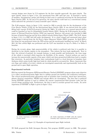
1.2 Examples of experimental space flight testbeds . . . . . . . . . . . . . . . . . . . . . . . . 2
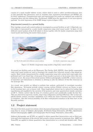
1.3 Double compression ramp models a flap-body control surface . . . . . . . . . . . . . . . . 3
2.1 Overview of the HTFD . . . . . . . . . . . . . . . . . . . . . . . . . . . . . . . . . . . . . . 5
2.2 Tamdem nozzle of the HTFD. Figure taken from Schrijer [2010a] . . . . . . . . . . . . . . 7
2.3 The undisturbed flow region in the test section [Schrijer, 2010a, Schrijer and Bannink, 2008] 8
2.4 Double compression ramp designs . . . . . . . . . . . . . . . . . . . . . . . . . . . . . . . . 9
2.5 Double compression ramp model located in the test section of the HTFD. Image taken
from Caljouw [2007] . . . . . . . . . . . . . . . . . . . . . . . . . . . . . . . . . . . . . . . 10
2.6 Design plot of the boundary layer thickness against the wedge angle (θ) and the wedge
length (L) [Ekelschot, 2012] . . . . . . . . . . . . . . . . . . . . . . . . . . . . . . . . . . . 11
2.7 Top view of the double compression ramp with Mach waves and the undisturbed region
(grey) . . . . . . . . . . . . . . . . . . . . . . . . . . . . . . . . . . . . . . . . . . . . . . . 11
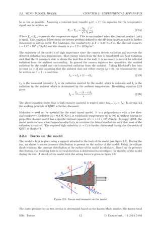
2.8 Forces and moment on the model . . . . . . . . . . . . . . . . . . . . . . . . . . . . . . . . 12
2.9 Sketch of the zig-zag VG and the model with corresponding coordinate systems . . . . . . 14
2.10 Determination of the radius of curvature and G¨ortler number . . . . . . . . . . . . . . . . 14
3.1 Graphical representation of Snell’s law . . . . . . . . . . . . . . . . . . . . . . . . . . . . . 16
3.2 Set-up of the Schlieren system in the HTFD. Figure taken from Schrijer [2010a] . . . . . . 16
3.3 General working principle of Schlieren photography . . . . . . . . . . . . . . . . . . . . . . 16
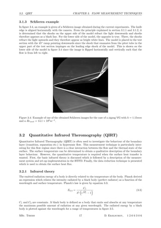
3.4 Example of one of the obtained Schlieren images for the case of a zigzag VG with h =
1.15mm and a Reunit = 14.1 × 106
m−1
. . . . . . . . . . . . . . . . . . . . . . . . . . . . . 17
3.5 Planck’s law (blue lines) and Wien’s law (red line) . . . . . . . . . . . . . . . . . . . . . . 18
3.6 radiant thermal budget. Figure taken from Scarano [2007] . . . . . . . . . . . . . . . . . . 18
3.7 The CEDIP camera . . . . . . . . . . . . . . . . . . . . . . . . . . . . . . . . . . . . . . . 20
3.8 The two FOVs for the test case hzz = 1.15 mm and Reunit = 14.1 × 106
[m−1
] . . . . . . . 20
3.9 The camera set-up with respect to the test section and the model during a QIRT experiment
and the variation in directional emissivity for several electrical nonconductors [Scarano,
2007] . . . . . . . . . . . . . . . . . . . . . . . . . . . . . . . . . . . . . . . . . . . . . . . . 21
3.10 The measured data at a local point in the measurement plane (xpix, ypix) = (150, 150) . . 21
3.11 Schematic representation of the working principle of a 2C-PIV experiment. Figure taken
from Schrijer [2010a] . . . . . . . . . . . . . . . . . . . . . . . . . . . . . . . . . . . . . . . 23
3.12 Cyclone seeder. . . . . . . . . . . . . . . . . . . . . . . . . . . . . . . . . . . . . . . . . . . 24
3.13 Particle velocity plotted together with the velocity of the fluid passing through a shock . . 25
3.14 Scanning Electron Microscope (SEM) images of the TiO2 50 nm particle tracers. Figures
taken from Schrijer et al. [2005] . . . . . . . . . . . . . . . . . . . . . . . . . . . . . . . . . 25
3.15 The laser set-up . . . . . . . . . . . . . . . . . . . . . . . . . . . . . . . . . . . . . . . . . . 26
3.16 2D cross correlation procedure . . . . . . . . . . . . . . . . . . . . . . . . . . . . . . . . . 27
3.17 graphical representation of window deformation . . . . . . . . . . . . . . . . . . . . . . . . 28
3.18 Block diagram of the iterative image deformation interrogation method . . . . . . . . . . 29
3.19 Schematic representation of the working principle of a Tomo-PIV experiment [Elsinga, 2008] 29
3.20 Plate calibration procedure . . . . . . . . . . . . . . . . . . . . . . . . . . . . . . . . . . . 30
3.21 Schematic representation of the triangulation error. Figure taken from Wieneke [2008]. . . 31
iv

9. LIST OF FIGURES LIST OF FIGURES
3.22 Summed disparity map over 1 - 16 images [Wieneke, 2008] . . . . . . . . . . . . . . . . . . 31
3.23 Ghost particles seen by the recording system [Novara et al., 2010] . . . . . . . . . . . . . . 33
3.24 Quality factor plotted against ppp and viewing angle θ figures are all taken from Elsinga
[2008] . . . . . . . . . . . . . . . . . . . . . . . . . . . . . . . . . . . . . . . . . . . . . . . 34
4.1 Flow topology for a single compression ramp. Figure taken from Arnal and Delery [2004] 36
4.2 Typical laminar boundary layer profile compared to a typical separated boundary layer
profile . . . . . . . . . . . . . . . . . . . . . . . . . . . . . . . . . . . . . . . . . . . . . . . 37
4.3 Instantaneous schlieren image for the case hzz = 0mm and Re = 8.47 × 106
m−1
. . . . . . 38
4.4 Instantaneous schlieren image for the case hzz = 1.15mm and Re = 8.47 × 106
m−1
. . . . 39
4.5 Sketch of the 5◦
− 45◦
model . . . . . . . . . . . . . . . . . . . . . . . . . . . . . . . . . . 40
4.6 Overview of the domain of interest during the PIV measurement campaign . . . . . . . . 41
4.7 Converging mean of Vx at a local data point in the free stream . . . . . . . . . . . . . . . 42
4.8 Macroscopic flow overview by means of a contour map for Vtot. Vtot is given in m/s . . . 42
4.9 Leading edge shock and separation shock indicated by the colormap of the Vy. Vy is given
in m/s . . . . . . . . . . . . . . . . . . . . . . . . . . . . . . . . . . . . . . . . . . . . . . . 43
4.10 Detailed colormap of the flow angle on the 45◦
ramp. Flow angle is given in degrees . . . 43
4.11 Detail of the separation bubble upstream of the hinge line of the model. Vtot is given in m/s 44
4.12 Recirculation bubble near the hinge line of the model. Vtot is given in m/s . . . . . . . . . 45
4.13 Detailed velocity field behind the bow shock on the 45◦
ramp. Vtot is given in m/s . . . . 45
4.14 The boundary layer thickness plotted against the streamwise coordinate s . . . . . . . . . 47
4.15 Comparison between the measured ch on the 5◦
ramp and ch determined by the Reference
Temperature Method . . . . . . . . . . . . . . . . . . . . . . . . . . . . . . . . . . . . . . . 48
4.16 Example of a streamwise Stanton number distribution for the case of hzz = 0, Re =
14.1 × 106
[m−1
] . . . . . . . . . . . . . . . . . . . . . . . . . . . . . . . . . . . . . . . . . 49
4.17 The logarithm of the Stanton number (ch) mapped on the surface coordinate system for
the case hzz = 0mm, Re = 14.1 × 106
m−1
. . . . . . . . . . . . . . . . . . . . . . . . . . 50
4.18 Expected flow topology behind a zig-zag VG . . . . . . . . . . . . . . . . . . . . . . . . . 50
4.19 Evolution of the secondary instability [Saric, 1994] . . . . . . . . . . . . . . . . . . . . . . 51
4.20 The expected Vy and Vz distribution together with the expected surface heat flux . . . . . 52
4.21 Results regarding the flow topology around zig-zag in subsonic flow by Elsinga and West-
erweel [2012] . . . . . . . . . . . . . . . . . . . . . . . . . . . . . . . . . . . . . . . . . . . 52
4.22 Results regarding the flow topology around zig-zag in subsonic flow by Sch¨ulein and Trofi-
mov [2011] . . . . . . . . . . . . . . . . . . . . . . . . . . . . . . . . . . . . . . . . . . . . . 53
4.23 Instable flow situation causing the G¨ortler instability. Figure taken from Saric [1994] . . . 54
4.24 Sketch of G¨ortler vortices in a boundary layer and a sketch of the model with cylindrical
coordinate system . . . . . . . . . . . . . . . . . . . . . . . . . . . . . . . . . . . . . . . . 55
4.25 Stability plot [Ekelschot, 2012] . . . . . . . . . . . . . . . . . . . . . . . . . . . . . . . . . 56
4.26 PIV results obtained by Schrijer [2010a] . . . . . . . . . . . . . . . . . . . . . . . . . . . . 57
4.27 Growth rate plotted against the G¨ortler number for three different wavelengths for the two
configurations presently discussed [Schrijer, 2010b] . . . . . . . . . . . . . . . . . . . . . . 58
4.28 G¨ortler number plotted against the wavelength parameter for the two configurations presently
discused [Schrijer, 2010b] . . . . . . . . . . . . . . . . . . . . . . . . . . . . . . . . . . . . 59
4.29 Test case presented in Luca de et al. [1993] . . . . . . . . . . . . . . . . . . . . . . . . . . 59
5.1 The mapped heat transfer distributions for all the tested Reynolds numbers and hzz =
1.15mm . . . . . . . . . . . . . . . . . . . . . . . . . . . . . . . . . . . . . . . . . . . . . . 62
5.2 Filtering procedure illustrated for hzz = 1.15 mm and Reunit = 14.1 × 106
[m−1
] . . . . . 62
5.3 The effect of the Reynolds number on the stream wise heat transfer distribution for all hzz. 64
5.4 The effect of the Reynolds number on the spanwise heat transfer distribution at fixed x
for all hzz . . . . . . . . . . . . . . . . . . . . . . . . . . . . . . . . . . . . . . . . . . . . . 65
5.5 Noise level comparison . . . . . . . . . . . . . . . . . . . . . . . . . . . . . . . . . . . . . . 67
5.6 Growth rate plotted in x direction for all hzz . . . . . . . . . . . . . . . . . . . . . . . . . 68
5.7 Example of initial disturbance . . . . . . . . . . . . . . . . . . . . . . . . . . . . . . . . . . 68
5.8 Examples of secondary disturbance amplification . . . . . . . . . . . . . . . . . . . . . . . 69
5.9 Example of obtaining the spanwise wavelength by means of autocorrelation . . . . . . . . 70
5.10 Correlation analysis of the spanwise heat transfer fluctuations . . . . . . . . . . . . . . . . 70
5.11 Growth rate plotted in x direction for all hzz . . . . . . . . . . . . . . . . . . . . . . . . . 71
MSc. Thesis v D. Ekelschot, 1 2 6 6 3 0 6

10. LIST OF FIGURES LIST OF FIGURES
5.12 Comparison of the spanwise surface heat flux at three different locations for hzz = 0.20
mm and hzz = 1.15 mm . . . . . . . . . . . . . . . . . . . . . . . . . . . . . . . . . . . . . 72
6.1 Sketch of the double compression ramp with the FOVs . . . . . . . . . . . . . . . . . . . . 74
6.2 Overview of the Tomo-PIV set-up in the HTFD for the first FOV . . . . . . . . . . . . . . 75
6.3 Camera orientation with respect to the measurement domain . . . . . . . . . . . . . . . . 76
6.4 Overview of the Tomo-PIV set-up in the HTFD for the first FOV . . . . . . . . . . . . . . 76
6.5 Laser sheet orientation for both measurements parallel to first and parallel to the 45◦
ramp 77
6.6 The mean Intensity plotted in z direction to check the sheet thickness . . . . . . . . . . . 78
6.7 Graphical representation of the refractive effect . . . . . . . . . . . . . . . . . . . . . . . . 79
6.8 Three dimensional theoretical error estimation due to the refractive effect . . . . . . . . . 80
6.9 Experimentally determined pixel shift for the three camera set-up used for FOV 1 . . . . 80
6.10 Graphical representation of the pixel shift caused by a tilted refractive interface . . . . . . 81
6.11 Pixel shift induced by the tilting of the window . . . . . . . . . . . . . . . . . . . . . . . . 82
6.12 Determination of the ppp . . . . . . . . . . . . . . . . . . . . . . . . . . . . . . . . . . . . 83
6.13 Measurement accuracy assessment for FOV 1 . . . . . . . . . . . . . . . . . . . . . . . . . 85
6.14 Measurement accuracy assessment for FOV 2 . . . . . . . . . . . . . . . . . . . . . . . . . 86
6.15 Correlation factor in x, y, z based on the reconstructed particle distribution . . . . . . . . 87
6.16 General 3D flow overview . . . . . . . . . . . . . . . . . . . . . . . . . . . . . . . . . . . . 88
6.17 General 3D flow overview . . . . . . . . . . . . . . . . . . . . . . . . . . . . . . . . . . . . 89
6.18 Flow overview parallel to the 5◦
ramp. Velocity magnitude is given in m/s . . . . . . . . 90
6.19 Contour map Vx parallel to the 5◦
ramp . . . . . . . . . . . . . . . . . . . . . . . . . . . . 90
6.20 Contour map Vz parallel to the 5◦
ramp . . . . . . . . . . . . . . . . . . . . . . . . . . . . 90
6.21 The spanwise v
y and v
z distribution for four fixed x positions . . . . . . . . . . . . . . . . 91
6.22 Contour map of Vx with its corresponding contour map v
y for four different fixed streamwise
positions on the 5◦
ramp . . . . . . . . . . . . . . . . . . . . . . . . . . . . . . . . . . . . . 93
6.23 Flow overview parallel to the 45◦
ramp. Velocity magnitude is given in m/s . . . . . . . . 94
6.24 The mean streamwise Vx velocity distribution parallel to the 45◦
ramp . . . . . . . . . . . 94
6.25 The mean streamwise Vz velocity distribution parallel to the 45◦
ramp . . . . . . . . . . . 95
6.26 Contour map for Vx and Vz for four fixed z positions parallel to the 45◦
ramp . . . . . . . 96
6.27 Spanwise velocity perturbations v
y and v
z for four fixed x positions . . . . . . . . . . . . . 97
6.28 Contour map of the velocity perturbations v
y and v
z for four fixed z positions . . . . . . . 98
A.1 Sample of a raw PIV images and the corresponding mean velocity field for the first FOV . 106
A.2 Sample of a raw PIV images and the corresponding mean velocity field for the second FOV 107
A.3 Sample of a raw PIV images and the corresponding mean velocity field for the third FOV 108
C.1 The Stanton number (ch) plotted on the physical model coordinates for the three Reynolds
numbers and hzz = 0 mm . . . . . . . . . . . . . . . . . . . . . . . . . . . . . . . . . . . . 112
C.2 The Stanton number (ch) plotted on the physical model coordinates for the three Reynolds
numbers and hzz = 0.20 mm . . . . . . . . . . . . . . . . . . . . . . . . . . . . . . . . . . 113
C.3 The Stanton number (ch) plotted on the physical model coordinates for the three Reynolds
numbers and hzz = 0.40 mm . . . . . . . . . . . . . . . . . . . . . . . . . . . . . . . . . . 114
C.4 The Stanton number (ch) plotted on the physical model coordinates for the three Reynolds
numbers and hzz = 0.75 mm . . . . . . . . . . . . . . . . . . . . . . . . . . . . . . . . . . 115
C.5 The Stanton number (ch) plotted on the physical model coordinates for the three Reynolds
numbers and hzz = 1.15 mm . . . . . . . . . . . . . . . . . . . . . . . . . . . . . . . . . . 116
D.1 Typical disparity map for the three different cameras . . . . . . . . . . . . . . . . . . . . . 117
E.1 Contour map of Vx with its corresponding contour map stdVx
for four different fixed stream-
wise positions on the 5◦
ramp . . . . . . . . . . . . . . . . . . . . . . . . . . . . . . . . . . 119
MSc. Thesis vi D. Ekelschot, 1 2 6 6 3 0 6

11. List of Tables
2.1 Total quantities in the test section depending on the nozzle. The values are taken from
Schrijer [2010a] . . . . . . . . . . . . . . . . . . . . . . . . . . . . . . . . . . . . . . . . . . 9
3.1 Number of vectors in x and y direction during the performed 2C-PIV measurements in the
HTFD . . . . . . . . . . . . . . . . . . . . . . . . . . . . . . . . . . . . . . . . . . . . . . . 28
4.1 Local Mach number for all domains . . . . . . . . . . . . . . . . . . . . . . . . . . . . . . . 40
4.2 Local Mach number for all domains . . . . . . . . . . . . . . . . . . . . . . . . . . . . . . . 46
4.3 Flow conditions behind the leading edge shock . . . . . . . . . . . . . . . . . . . . . . . . 47
4.4 Dimensions of the two tested configurations test by Schrijer [2010b,a] . . . . . . . . . . . . 57
4.5 Dimensions of the two tested configurations test by Luca de et al. [1993] . . . . . . . . . . 58
5.1 Test matrix . . . . . . . . . . . . . . . . . . . . . . . . . . . . . . . . . . . . . . . . . . . . 61
6.1 Geometrical characteristics of the measurement set-up parallel to the 5◦
ramp . . . . . . . 75
6.2 Geometrical characteristics of the measurement set-up parallel to the 45◦
ramp . . . . . . 77
6.3 Pixel shift . . . . . . . . . . . . . . . . . . . . . . . . . . . . . . . . . . . . . . . . . . . . . 80
6.4 Geometrical characteristics of the measurement set-up parallel to the 5◦
ramp . . . . . . . 83
6.5 Number of vectors . . . . . . . . . . . . . . . . . . . . . . . . . . . . . . . . . . . . . . . . 84
6.6 Standard deviation and mean for every velocity component in the (y1, z1) plane for the
presented test case . . . . . . . . . . . . . . . . . . . . . . . . . . . . . . . . . . . . . . . . 85
6.7 Standard deviation and mean for every velocity component in the (y, z) plane for the
presented test case . . . . . . . . . . . . . . . . . . . . . . . . . . . . . . . . . . . . . . . . 86
7.1 Standard deviation and mean for every velocity component in the (y, z) plane for the
presented test case . . . . . . . . . . . . . . . . . . . . . . . . . . . . . . . . . . . . . . . . 102
7.2 Standard deviation and mean for every velocity component in the (y, z) plane for the
presented test case . . . . . . . . . . . . . . . . . . . . . . . . . . . . . . . . . . . . . . . . 102
vii

12. List of Symbols
x Longitudinal coordinate [mm]. . . . . . . . . . . . . . . . . . . . . . . . . . . . . . . . . . . . . . . . . . . . . . . . . . . . . . . . . . . . . . . . . . .5
y Spanwise coordinate [mm] . . . . . . . . . . . . . . . . . . . . . . . . . . . . . . . . . . . . . . . . . . . . . . . . . . . . . . . . . . . . . . . . . . . . .14
z Normal coordinate [mm] . . . . . . . . . . . . . . . . . . . . . . . . . . . . . . . . . . . . . . . . . . . . . . . . . . . . . . . . . . . . . . . . . . . . . . 14
x1 Streamwise coordinate tangent to the 5◦
ramp [mm] . . . . . . . . . . . . . . . . . . . . . . . . . . . . . . . . . . . . . . . . . . .14
y1 Spanwise coordinate defined at the hinge line at the 5◦
ramp [mm] . . . . . . . . . . . . . . . . . . . . . . . . . . . . 14
z1 Normal coordinate at the 5◦
ramp [mm] . . . . . . . . . . . . . . . . . . . . . . . . . . . . . . . . . . . . . . . . . . . . . . . . . . . . . . .14
x2 Streamwise coordinate tangent to the 45◦
ramp [mm] . . . . . . . . . . . . . . . . . . . . . . . . . . . . . . . . . . . . . . . . . 14
y2 Spanwise coordinate defined at the hinge line at the 45◦
ramp [mm] . . . . . . . . . . . . . . . . . . . . . . . . . . . 14
z2 Normal coordinate at the 45◦
ramp [mm] . . . . . . . . . . . . . . . . . . . . . . . . . . . . . . . . . . . . . . . . . . . . . . . . . . . . . 14
θ Ramp angle [◦
] . . . . . . . . . . . . . . . . . . . . . . . . . . . . . . . . . . . . . . . . . . . . . . . . . . . . . . . . . . . . . . . . . . . . . . . . . . . . . . . .14
t Time [s] . . . . . . . . . . . . . . . . . . . . . . . . . . . . . . . . . . . . . . . . . . . . . . . . . . . . . . . . . . . . . . . . . . . . . . . . . . . . . . . . . . . . . . . .5
a Speed of sound [m/s] . . . . . . . . . . . . . . . . . . . . . . . . . . . . . . . . . . . . . . . . . . . . . . . . . . . . . . . . . . . . . . . . . . . . . . . . . . .6
γ Specific heat ratio [-] . . . . . . . . . . . . . . . . . . . . . . . . . . . . . . . . . . . . . . . . . . . . . . . . . . . . . . . . . . . . . . . . . . . . . . . . . . . 6
M Mach number [-] . . . . . . . . . . . . . . . . . . . . . . . . . . . . . . . . . . . . . . . . . . . . . . . . . . . . . . . . . . . . . . . . . . . . . . . . . . . . . . . 6
A Cross sectional area [mm2
] . . . . . . . . . . . . . . . . . . . . . . . . . . . . . . . . . . . . . . . . . . . . . . . . . . . . . . . . . . . . . . . . . . . . . 7
d Diameter [mm] . . . . . . . . . . . . . . . . . . . . . . . . . . . . . . . . . . . . . . . . . . . . . . . . . . . . . . . . . . . . . . . . . . . . . . . . . . . . . . . . .7
p Pressure [Pa] . . . . . . . . . . . . . . . . . . . . . . . . . . . . . . . . . . . . . . . . . . . . . . . . . . . . . . . . . . . . . . . . . . . . . . . . . . . . . . . . . . 7
pt Total pressure [Pa] . . . . . . . . . . . . . . . . . . . . . . . . . . . . . . . . . . . . . . . . . . . . . . . . . . . . . . . . . . . . . . . . . . . . . . . . . . . . .8
T Temperature [K] . . . . . . . . . . . . . . . . . . . . . . . . . . . . . . . . . . . . . . . . . . . . . . . . . . . . . . . . . . . . . . . . . . . . . . . . . . . . . . . 8
Tt Total temperature [K] . . . . . . . . . . . . . . . . . . . . . . . . . . . . . . . . . . . . . . . . . . . . . . . . . . . . . . . . . . . . . . . . . . . . . . . . . .8
Tw Wall temperature [K] . . . . . . . . . . . . . . . . . . . . . . . . . . . . . . . . . . . . . . . . . . . . . . . . . . . . . . . . . . . . . . . . . . . . . . . . . 22
ρ∞ Free stream density [-] . . . . . . . . . . . . . . . . . . . . . . . . . . . . . . . . . . . . . . . . . . . . . . . . . . . . . . . . . . . . . . . . . . . . . . . . 22
µ∞ Viscosity [mm] . . . . . . . . . . . . . . . . . . . . . . . . . . . . . . . . . . . . . . . . . . . . . . . . . . . . . . . . . . . . . . . . . . . . . . . . . . . . . . . . 47
R Gas constant [ J
mol·K ] . . . . . . . . . . . . . . . . . . . . . . . . . . . . . . . . . . . . . . . . . . . . . . . . . . . . . . . . . . . . . . . . . . . . . . . . . . . 8
cp Specific heat [ J
kg·K ] . . . . . . . . . . . . . . . . . . . . . . . . . . . . . . . . . . . . . . . . . . . . . . . . . . . . . . . . . . . . . . . . . . . . . . . . . . . . .8
haw Enthalpy at a adiabatic wall [ J
kg ] . . . . . . . . . . . . . . . . . . . . . . . . . . . . . . . . . . . . . . . . . . . . . . . . . . . . . . . . . . . . . . 22
hw Enthalphy at the wall [ J
kg ] . . . . . . . . . . . . . . . . . . . . . . . . . . . . . . . . . . . . . . . . . . . . . . . . . . . . . . . . . . . . . . . . . . . . 22
L1 Tangent length of the first ramp [mm] . . . . . . . . . . . . . . . . . . . . . . . . . . . . . . . . . . . . . . . . . . . . . . . . . . . . . . . . .14
L2 Tangent length of the second ramp [mm] . . . . . . . . . . . . . . . . . . . . . . . . . . . . . . . . . . . . . . . . . . . . . . . . . . . . . . 14
hzz Height of the VG [mm] . . . . . . . . . . . . . . . . . . . . . . . . . . . . . . . . . . . . . . . . . . . . . . . . . . . . . . . . . . . . . . . . . . . . . . . .10
λzz Spanwise wavelength of the VG [mm] . . . . . . . . . . . . . . . . . . . . . . . . . . . . . . . . . . . . . . . . . . . . . . . . . . . . . . . . . 61
G G¨ortler number [-] . . . . . . . . . . . . . . . . . . . . . . . . . . . . . . . . . . . . . . . . . . . . . . . . . . . . . . . . . . . . . . . . . . . . . . . . . . . . 10
σ Growth rate [-] . . . . . . . . . . . . . . . . . . . . . . . . . . . . . . . . . . . . . . . . . . . . . . . . . . . . . . . . . . . . . . . . . . . . . . . . . . . . . . . .66
β Non dimensional wave number [-] . . . . . . . . . . . . . . . . . . . . . . . . . . . . . . . . . . . . . . . . . . . . . . . . . . . . . . . . . . . . . .56
n Refraction index [-] . . . . . . . . . . . . . . . . . . . . . . . . . . . . . . . . . . . . . . . . . . . . . . . . . . . . . . . . . . . . . . . . . . . . . . . . . . . .15
ϕ Rotational angle around the x-axis [◦
] . . . . . . . . . . . . . . . . . . . . . . . . . . . . . . . . . . . . . . . . . . . . . . . . . . . . . . . . . 74
θ Rotational angle around the y-axis [◦
] . . . . . . . . . . . . . . . . . . . . . . . . . . . . . . . . . . . . . . . . . . . . . . . . . . . . . . . . . 74
ω Rotational angle around the z-axis [◦
] . . . . . . . . . . . . . . . . . . . . . . . . . . . . . . . . . . . . . . . . . . . . . . . . . . . . . . . . . 74
v Velocity vector [-] . . . . . . . . . . . . . . . . . . . . . . . . . . . . . . . . . . . . . . . . . . . . . . . . . . . . . . . . . . . . . . . . . . . . . . . . . . . . . 27
V x Velocity component in the defined x direction [m/s] . . . . . . . . . . . . . . . . . . . . . . . . . . . . . . . . . . . . . . . . . . . 91
V y Velocity component in the defined y direction [m/s] . . . . . . . . . . . . . . . . . . . . . . . . . . . . . . . . . . . . . . . . . . . 91
V z Velocity component in the defined z direction [m/s] . . . . . . . . . . . . . . . . . . . . . . . . . . . . . . . . . . . . . . . . . . . 91
v
x Velocity fluctuation in the defined x direction [m/s] . . . . . . . . . . . . . . . . . . . . . . . . . . . . . . . . . . . . . . . . . . . 91
v
y Velocity fluctuation in the defined y direction [m/s] . . . . . . . . . . . . . . . . . . . . . . . . . . . . . . . . . . . . . . . . . . . 91
v
z Velocity fluctuation in the defined z direction [m/s] . . . . . . . . . . . . . . . . . . . . . . . . . . . . . . . . . . . . . . . . . . . 91
Re
m Unit reynolds number [ 1
m ] . . . . . . . . . . . . . . . . . . . . . . . . . . . . . . . . . . . . . . . . . . . . . . . . . . . . . . . . . . . . . . . . . . . . . . 8
emissivity [-] . . . . . . . . . . . . . . . . . . . . . . . . . . . . . . . . . . . . . . . . . . . . . . . . . . . . . . . . . . . . . . . . . . . . . . . . . . . . . . . . . . 10
viii

13. LIST OF TABLES LIST OF TABLES
I Particle intensity [-] . . . . . . . . . . . . . . . . . . . . . . . . . . . . . . . . . . . . . . . . . . . . . . . . . . . . . . . . . . . . . . . . . . . . . . . . . . . 27
Ntot Total number of pixels [-] . . . . . . . . . . . . . . . . . . . . . . . . . . . . . . . . . . . . . . . . . . . . . . . . . . . . . . . . . . . . . . . . . . . . . 28
ppp Particle Per Pixel [-] . . . . . . . . . . . . . . . . . . . . . . . . . . . . . . . . . . . . . . . . . . . . . . . . . . . . . . . . . . . . . . . . . . . . . . . . . . 28
ppv Particle Per Voxel [-] . . . . . . . . . . . . . . . . . . . . . . . . . . . . . . . . . . . . . . . . . . . . . . . . . . . . . . . . . . . . . . . . . . . . . . . . . . 78
αi,j Pixel gain [-] . . . . . . . . . . . . . . . . . . . . . . . . . . . . . . . . . . . . . . . . . . . . . . . . . . . . . . . . . . . . . . . . . . . . . . . . . . . . . . . . . . 19
βi,j Pixel offset [-] . . . . . . . . . . . . . . . . . . . . . . . . . . . . . . . . . . . . . . . . . . . . . . . . . . . . . . . . . . . . . . . . . . . . . . . . . . . . . . . . . 19
Ue Total velocity at the edge of the boundary layer [m/s] . . . . . . . . . . . . . . . . . . . . . . . . . . . . . . . . . . . . . . . . . 22
St Stanton number [-] . . . . . . . . . . . . . . . . . . . . . . . . . . . . . . . . . . . . . . . . . . . . . . . . . . . . . . . . . . . . . . . . . . . . . . . . . . . . 22
ch Stanton number [-] . . . . . . . . . . . . . . . . . . . . . . . . . . . . . . . . . . . . . . . . . . . . . . . . . . . . . . . . . . . . . . . . . . . . . . . . . . . . 22
Cf Friction coefficient [-] . . . . . . . . . . . . . . . . . . . . . . . . . . . . . . . . . . . . . . . . . . . . . . . . . . . . . . . . . . . . . . . . . . . . . . . . . .46
qs Heat transfer [−k ∂T
∂y ] . . . . . . . . . . . . . . . . . . . . . . . . . . . . . . . . . . . . . . . . . . . . . . . . . . . . . . . . . . . . . . . . . . . . . . . . . .22
δ Boundary layer thickness [mm] . . . . . . . . . . . . . . . . . . . . . . . . . . . . . . . . . . . . . . . . . . . . . . . . . . . . . . . . . . . . . . . . 47
d Disparity vector [pix] . . . . . . . . . . . . . . . . . . . . . . . . . . . . . . . . . . . . . . . . . . . . . . . . . . . . . . . . . . . . . . . . . . . . . . . . . .31
¯σ Disparity vector [pix] . . . . . . . . . . . . . . . . . . . . . . . . . . . . . . . . . . . . . . . . . . . . . . . . . . . . . . . . . . . . . . . . . . . . . . . . . .84
Nr Number of runs [-] . . . . . . . . . . . . . . . . . . . . . . . . . . . . . . . . . . . . . . . . . . . . . . . . . . . . . . . . . . . . . . . . . . . . . . . . . . . . 84
voxx Number of voxels in x direction [-] . . . . . . . . . . . . . . . . . . . . . . . . . . . . . . . . . . . . . . . . . . . . . . . . . . . . . . . . . . . . 34
voxy Number of voxels in y direction [-] . . . . . . . . . . . . . . . . . . . . . . . . . . . . . . . . . . . . . . . . . . . . . . . . . . . . . . . . . . . . .34
voxz Number of voxels in z direction [-] . . . . . . . . . . . . . . . . . . . . . . . . . . . . . . . . . . . . . . . . . . . . . . . . . . . . . . . . . . . . .34
MSc. Thesis ix D. Ekelschot, 1 2 6 6 3 0 6

14. Abstract
Aerodynamic heating is one of the driving aspects in hypersonic vehicle design. During take-off and
re-entry, high heat loads are encountered for which the appropriate measures have to be considered. In
particular during the re-entry phase, high maneuverability of the vehicle is preferred such that reusable
(manned) spacecraft can land on conventional runways. Control devices are therefore a necessity to im-
prove the maneuverability of the spacecraft. Consequently, the hypersonic flow behaviour around control
flaps is thoroughly investigated over the last decades. Boundary layer separation/reattachment and shock
wave interaction are general flow phenomena that occur in hypersonic double ramp flow. Furthermore,
streamwise periodic counter rotating vortices (G¨ortler vortices) tend to grow in the boundary layer over
the control surface. G¨ortler vortices are induced by the centrifugal forces associated with the change in
direction of motion forced on the fluid by the concave geometry of the surface. G¨ortler vortices take the
form of a striation pattern and considerably modify the heat flux and can cause spanwise heat transfer
variations of 100%.
An experimental study is performed in the Hypersonic Test Facility Delft (HTFD) using a scaled dou-
ble compression ramp wind tunnel model that represents a flap body control surface. A zig-zag Vortex
Generator (VG) is pasted near the leading edge of the model to ensure that steady spanwise periodic
longitudinal structures are present in the boundary layer. In this way a controlled investigation is per-
formed on the amplification of longitudinal vortices due to the concave geometry of the model.
During this thesis project, Quantitative Infrared Thermography (QIRT) and Tomographic Particle Image
Velocimetry (Tomo-PIV) measurements are performed to investigate the development of G¨ortler vortices
in hypersonic double compression ramp flow at Mach 7.5. QIRT is used to obtain results regarding the
growth rate of G¨ortler vortices while Tomo-PIV gives more insight on the local three dimensional flow
behaviour. Therefore the concave wind tunnel model also serves as a initial test case to verify whether
Tomo-PIV is applicable in the (Hypersonic Test Facility Delft) HTFD.
A 5◦
− 45◦
double compression ramp model is tested with L1 = 150mm and L2 = 80.9mm where
L1 and L2 are the tangent wedge lengths of the 5◦
and 45◦
ramp, respectively.
(a) The investigated windtunnel model (b) Sketch of the zig-zag Vortex Generator
Figure 1: Sketch of the investigated windtunnel model and a sketch of the zig-zag Vortex Generator (VG)
The influence of the height of the zig-zag strip (hzz) and the Reynolds number on the amplifica-
tion of these longitudinal structures is investigated. The wavelength of the VG (λV G = 6 mm) and
the streamwise width (wzz = 11 mm) are fixed and the height is varied within the given range of
x

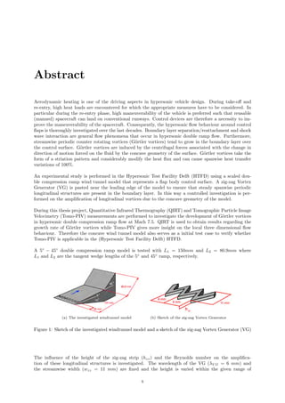
15. CHAPTER 0. ABSTRACT
hzz = [0, 0.20, 0.40, 0.75, 1.15] mm. Measurements are performed at three unit Reynolds numbers,
Reunit = 8.47 × 106
[m−1
], Reunit = 11.3 × 106
[m−1
] and Reunit = 14.1 × 106
[m−1
]. The VG is lo-
cated at 2.5mm from the leading edge of the model.
Initially, a Schlieren photography measurement campaign is performed to obtain the stability and topol-
ogy of the shock pattern which is useful for supporting and providing a better understanding of the
obtained QIRT and Tomo-PIV results. The flow topology and shock interactions due to the geometry of
the model are used to determine the local flow properties by determining the corresponding hodograph.
The theoretical analysis based on the quantitative flow overview is used to ascribe local flow behaviour
measured during the Tomo-PIV measurement campaign.
QIRT measurements are performed to obtain the heat flux distribution at the surface of the model.
Flow characteristics near the wall are obtained such as boundary layer separation and reattachment.
Furthermore, the spanwise heat flux distribution is investigated and based on the local spanwise fluctu-
ations induced by the V G, the growth rate of the longitudinal vortices is quantified. The effect of the
height of the V G and Reynolds number on the longitudinal vortex propagation is determined.
The QIRT results show a clear sinusoidal spanwise heat flux fluctuation with a wavelength that cor-
responds to λV G = 6mm. The influence of the Reynolds number on the heat transfer distribution is
investigated in local streamwise and spanwise direction. The streamwise thermograms indicate that
boundary layer separation occurs more downstream when the Reynolds number is increased. In spanwise
direction it is found that for the case of hzz = 1.15mm, the spanwise heat transfer fluctuations break up
into smaller streaks. The intensity of this behaviour is dependent on the Reynolds number. For some
test cases, the two dimensional heat transfer map shows a curved separation line which might be caused
due to a bad pasting of the VG.
The growth rate is quantified by the ratio of the spanwise heat transfer fluctuation at a local streamwise
position on the model and the spanwise heat transfer fluctuation at a fixed position near the leading
edge. Since the separation line is curved, it is chosen to locally investigate the growth rate of the G¨ortler
vortices. For all hzz it is found that the growth rate is below 1 on the 5◦
ramp which indicates that
the longitudinal structures dissipate in streamwise direction. The intensity of the spanwise heat transfer
fluctuations are again amplified on the 45◦
ramp. The growth rate reaches a local maximum of 15 for the
case hzz = 0.2 mm on the 45◦
while the maximum growth rate for the other cases is significantly lower
(±σ = 4). Furthermore a characteristic streamwise x − σ profile is found for all cases.
A detail 3D velocity field is obtained using Tomo-PIV. Experiments are performed for hzz = 1.15 mm
and Reunit = 14.1 × 106
[m−1
]. The 3D velocity field parallel to the 5◦
ramp and the 45◦
ramp is locally
measured by choosing 2 Field Of Views (FOV) of 60 mm × 40 mm × 6 mm. One FOV parallel to the
5◦
ramp and one parallel to the 45◦
.
The application of Tomo-PIV in the HTFD is verified. A flexible set-up is chosen such that both FOVs are
optically accessible. The model is placed in the test section such that the surface of the model is aligned
with the window of the tunnel. A laser sheet of approximately 6 mm thick is placed parallel to the 5◦
and 45◦
ramp such that the velocity field is measured approximately 2 mm above the surface of the model.
Due to the high convective streamwise velocity, difficulties are encountered for the measurement of the
out of plane velocity component. In both, the streamwise and spanwise velocity component, clear fluc-
tuations are measured. The fluctuations are rather small with respect to the local convective velocity
and in particular on the FOV parallel to the 5◦
ramp, the wakes induced by the VG are clearly visible.
The fluctuations in streamwise and spanwise velocity component are 10 m/s and 1 m/s, respectively.
Dividing the fluctuations by the corresponding convective velocity gives a 1 % fluctuation in Vx and a 10
% fluctuation in Vy. The out of plane velocity component shows a fluctuating spanwise behaviour which
is difficult to quantify. Furthermore, the in-depth resolution is lower since the velocity in this direction
is significantly lower (∆pixz = 2 pix) compared to the velocity in streamwise direction (∆pix = 30 pix).
Similar problems regarding the out of plane velocity component were encountered during the measure-
ment of the 3D velocity field parallel to the 45◦
ramp. Higher rms values were obtained during the
validation process, compared to the velocity field measurement parallel to the 5◦
ramp. This can be
MSc. Thesis xi D. Ekelschot, 1 2 6 6 3 0 6

16. CHAPTER 0. ABSTRACT
ascribed to the limited optical accessibility. Furthermore, the complex shock pattern that is located
above the 45◦
caused local particle blurring. This effect influences the quality of the reconstruction, and
therefore, the measurement outcome.
MSc. Thesis xii D. Ekelschot, 1 2 6 6 3 0 6

17. Chapter 1
Introduction
1.1 Background
Hypersonic research has been developing since the beginning of the 20th century after Konstantin Tsi-
olkovsky wrote The Exploration of cosmic space by means of reaction devices in 1903, in which he de-
scribed the general problems regarding rocket flight in space. It was soon found that the compressibility
of the flow brings new flow features to investigate such as aerothermaldynamic effects, shock wave inter-
action and shock wave boundary layer interaction (SWBLI).
(a) Space shuttle during the launch phase (b) Artist impression of the X-38 CVR
(c) Artist impression of the X-37 in re-entry phase
Figure 1.1: Maneuverable space vehicles
At first, knowledge about hypersonic aerodynamics was used for military purposes such as the V2 rocket
during the second world war. After the second world war, scientists developed an interest in creating
space programs which would eventually bring our society to where it is now. In particular during the cold
war, hypersonic investigation developed rapidly. Human space flight was realised and engineers came up
with concepts of a spacecraft which could return humans back to Earth from outer space. Initially this
has been done by using capsule shaped re-entry vehicles but later on, during the late 1970’s, the first
1

18. 1.1. BACKGROUND CHAPTER 1. INTRODUCTION
concept designs were drawn by U.S engineers for the first reusable spacecraft, the space shuttle. The
space shuttle, shown in figure 1.1(a), was operational from 1981 until last year. It launched a variety
of satellites, interplanetary probes and during its final years it conducted servicing for the International
Space Station (ISS). At the end of its operation, the space shuttle could land on a conventional runway
which indicated the potential of (semi)-reuseable space vehicles.
The X-38 program, shown in figure 1.1(b), started in 1995 to provide data for the development of the
Crew Return Vehicle (CVR) for the International Space Station (ISS). It was derived from the earlier
lifting body concept (X-23/X-24 projects) during the 1960’s. It could serve as a manned spacecraft that
could be launched on top of a Expandable Launch Vehicle (ELV). During the X-38 program the perfor-
mance of Thermal Protection System (TPS) was improved. However, this project was cancelled in 2002
because of limited financing and the focus shifted towards Orbital Space Planes (OSP). The X-37, shown
in figure 1.1(c), is a OSP and still under development. It is a short winged and unmanned space plane
whose design is derived from the Air Force’s Space Maneuver Vehicle (SMV) program. In April 2010 a
first drop test was performed where the TPS system and the aerodynamic handling was tested. In March
2011 the first orbital flight was performed and the X-37 was launched on top of a Delta 2 or Delta 4
launcher.
During the re-enrty phase, high maneuverability of the vehicle is preferred such that it is possible to
decelerate in low density regimes in the atmosphere. This reduces the heat loads significantly. Next to
that, the retrieval of payload, for example humans, is made possible and furthermore, the cross range
of the vehicle is increased which improves the flexibility of the mission. Control surfaces are used to
increase the maneuverable capacity of the space vehicle and these geometrical deflections lead to complex
flow structures. In particular boundary layer reattachment leads to a local decrease in boundary layer
thickness which causes locally high heat loads for which should be accounted for. Hence, hypersonic flow
over flaps and rudders of re-entry vehicles are investigated numerically and experimentally, both on the
ground and in space flight operation.
Experimental testbeds
ESA has started the European eXPErimental Reentry Testbed (EXPERT) program whose main objective
is to collect aerothermodynamic flight data to validate ground test facilities and verification techniques.
The critical aerothermodynamic phenomena such as boundary layer transition, shock layer interactions,
plasma chemical composition, SWBLI and real-gas effects are investigated. The data that is gathered
during EXPERT missions is used to validate the current computational fluid dynamic codes and the
current design modeling tools. Furthermore, the data is used to correlate ground test results. An artist
impression of EXPERT in flight is given in figure 1.2(a).
(a) Artist impression of EXPERT in
re-entry phase
Chapter 1
Introduction
1.1 Background
In the last century research in the field of high speed aerodynamics evolved from the development of ballistic
missiles in the early 1930s to the present space flight capabilities. Before and during the second world war
considerable effort was put into the development of rocket technology purely for military purposes. This was
the initiation of the era of space flight. After 1945 this development was continued by the U.S. and the Soviet-
Union during the period of the cold war. In the race for supremacy the development of high speed aerodynamics
evolved rapidly, what eventually led to the development of reusable launchers, such as the space shuttle.
In the 1980s, more advanced programs for reusable launchers were initiated, such as the Aero-Assisted Orbital
Transfer Vehicle (AOTV) in the U.S. and the HERMES project in Europe. These triggered the development
of more sophisticated numerical techniques to accurately predict the aerothermodynamic environment around
re-entry vehicles. To verify numerical computations, wind tunnel and flight experiments were performed to
validate these results (36).
reattachment shock
separation shock
separated shear layer
bow shock
Figure 1.1: Impression of hypersonic flow on
DART model
Because of developments in space flight, in 1999 the
DART project was initiated at the TU Delft. The DART
(Delft Aerospace Re-entry Test program) is a reusable re-
entry vehicle to provide testing and validation facilities at
hypersonic re-entry flight conditions (7). An impression of
the DART in hypersonic flow is given in figure 1.1. One
of the main goals of the present project was the collec-
tion of aerothermodynamic data in the hypersonic flight
regime. This data can used to validate theory and CFD
codes and to allow better interpretations of wind tunnel
measurements. The emphasis lays on separation and reat-
tachment of the boundary layer. An experimental investi-
gation on the flap effectiveness and the aerodynamic sur-
face heating of this model was done in the Hypersonic Test
Facility Delft (HTFD) (31). This investigation provided
substantial qualitative data on the flow situation and the
occurring heat loads.
Influenced by the DART project, ESA initiated the EX-
(b) Artist impression of DART with the typical
boundary layer separation and reattachment
Figure 1.2: Examples of experimental space flight testbeds
TU Delft proposed the Delft Aerospace Re-entry Test program (DART) project in 1999. The project
MSc. Thesis 2 D. Ekelschot, 1 2 6 6 3 0 6

19. 1.2. PROJECT STATEMENT CHAPTER 1. INTRODUCTION
consists of a small reusable ballistic re-enty vehicle which is used to collect aerothermodynamic data
so that particular flow phenomena, such as, boundary layer separation/reattachment and SWBLI, can
be better understood. Computational codes and experimental test results are validated and verified by
comparing them with the realtime data. Furthermore, DART gives the opportunity to test micro gravity
payloads. An artist impression of the DART design is given in figure 1.2(b).
Experimental research in a ground facility
Flow topology around such control surfaces is investigated on ground facilities as well. A flap-body con-
trol surface is represented by a scaled double compression ramp wind tunnel model. In figure 1.3 the
deflected control surfaces of the X-38 vehicle is shown together with the double compression ramp wind
tunnel model used during this master thesis project.
(a) The X-38 model with deflected control surfaces (b) Double compression ramp model
Figure 1.3: Double compression ramp models a flap-body control surface
At ground test facilities such as the Hypersonic Test Facility Delft (HTFD), these double compression
ramp wind tunnel models are used to investigate the complex flow behaviour around a flap shaped ge-
ometry. Heat transfer measurements for a double compression ramp with various back ramp angles were
performed and it was found that a local peak of heat transfer is present at the location where flow reat-
tachment occurs. By means of theoretical analysis, Schlieren photography and 2C-PIV, a better overview
of separation and reattachment is obtained, to allowing to infer the influence of this flow behaviour on
the isentropic flow.
As a result, new projects are defined to perform flow analysis, particularly to investigate secondary
flow phenomena. Streamwise periodic counter rotating vortices (G¨ortler vortices) are known to grow
in the boundary layer over a concave wall. These longitudinal vortices can be induced by leading edge
imperfections and amplified by the curvature of the geometry and cause spanwise heat transfer variations
of 100 %. G¨ortler vortices take the form of a striation pattern and considerably modify the heat flux.
They are observed in supersonic nozzles, swept wing configuration and flap deflections. Due to large am-
plitude G¨ortler vortices, secondary instabilities occur which may lead to boundary layer and transition
to turbulence. Also this vortical instability of the flow could promote transition in the shear layer at low
Reynolds numbers.
1.2 Project statement
The aim of this thesis project is to obtain a three dimensional impression of hypersonic double compression
ramp flow by means of Schlieren photography, 2C-Particle Image Velocimetry (2C-PIV), Quantitative
Infrared Thermography (QIRT) and Tomographic Particle Image Velocimetry (Tomo-PIV).
Schlieren photography and 2C-PIV are applied to obtain general flow characteristics such as shock pat-
terns and a first impression of the velocity field around a concave geometry in hypersonic flow. QIRT and
Tomo-PIV are applied to obtain quantitative flow characteristics at a overall and detailed scale. These
MSc. Thesis 3 D. Ekelschot, 1 2 6 6 3 0 6

20. 1.3. REPORT OUTLINE CHAPTER 1. INTRODUCTION
techniques are used to investigate G¨ortler vortices in hypersonic double compression ramp flow. The
validation and application of Tomographic Particle Image Velocimetry (Tomo-PIV) in the HTFD is a
significant part of the results of this thesis.
1.3 Report outline
This report is structured in seven chapters. In chapter 2, the experimental apparatus is discussed. The
reader is introduced with a description of the HTFD and the windtunnel model that is investigated during
this thesis project. The working principles of the applied flow measurement techniques are discussed in
chapter 3.
Chapter 4 consists of a general description of hypersonic double compression ramp flow. The flow anal-
ysis is shown for the geometry of the test model. Based on the theoretical analysis and the previously
performed literature study, a list of expected results is drawn. This chapter makes clear what the contri-
bution of this research project is with respect to the available literature.
Chapter 5 and 6 form the core part of this thesis report. The measurement campaigns together with the
corresponding measurement objectives are given. These chapters reveal the results which were found dur-
ing the experimental assessment phase of this project. In chapter 7, the conclusions and recommendations
are presented.
MSc. Thesis 4 D. Ekelschot, 1 2 6 6 3 0 6

21. Chapter 2
Experimental apparatus
In this chapter, the working principle of the Hypersonic Test Facility Delft (HTFD) is described. The
operational envelope is given and the reader is introduced to the free stream flow conditions that are
valid for the current experiments. Furthermore a detailed description is given of the wind tunnel model.
A list of model requirements is determined and further discussed in the last section of this chapter.
2.1 Description of Hypersonic Test Facility Delft (HTFD)
The Hypersonic Test Facility Delft (HTFD) is a Ludwieg tube concept tunnel. This concept relies on
the principle of a high pressure difference between the storage tube and the vacuum charge tank with a
fast acting valve upstream of the nozzle. When the valve is opened, the fluid flows from the storage tube
into the nozzle. The appropriate Mach number is set in the test section by changing the area ratio of the
nozzle with respect to the test section. In figure 2.1 a schematic representation of the operating principle
of HTFD is given together with a picture of the HTFD.
t
x
F
E
C
D
A
B
0
S
L
Storage tube
Fast acting valve
Nozzle
Test
section
Vacuum tank
Head wave
Tail wave
Particle
path
exp.
!L
p0 T0
pt
Ttp0 T0
p1 T1
t1
1
0
Figure 2.2: Operational principle of the Ludwieg tube
corresponding to a pressure ratio of:
pt,1
p0
=
1 + γ−1
2 M2
1
1 + γ−1
2 M1
2
γ
γ−1
(2.4)
The total running time of the facility with constant storage tube conditions is governed
by the time it takes before the reflected expansion wave reaches the fast acting valve.
It may be calculated from (see appendix A for the derivation):
t1 =
L
a0
2
1 + M1
1 +
γ − 1
2
M1
γ+1
2(γ−1)
(2.5)
The running time t1 is also represented in figure 2.2 by the time it takes for an
air particle going from condition 0 to E, where L is the length of the storage tube.
Finally the Mach number of the flow downstream of the expansion wave is determined
by imposing mass conservation, it depends directly on the tube diameter to the critical
throat diameter (denoted by the superscript *) ratio:
dtube
2
1
2
γ − 1
γ+1
2(γ−1)
(a) Operating principle of the HTFD
6 CHAPTER 2. HYPE
Figure 2.1: Overview (left) and test section (r
Tube length 29 m
Length ’hot’ tube 6 m
Length ’cold’ tube 23 m
Diameter ’hot’ tube 49.25
Diameter ’cold’ tube 59 mm
Length of facility 16 m
Nozzle opening angle 15◦
Test section diameter 35 cm
Maximum storage tube pressure 100 ba
Maximum storage tube temperature 825 K
Minimum pressure vacuum chamber 0.5 mb
Valve opening time ∼ 1 m
Vacuum chamber volume 3 m3
Vacuum pump performance 250 m
Gas (air) storage 0.2 m3
Compressor performance 0.14 m
(b) Picture of the HTFD
Figure 2.1: Overview of the HTFD
2.1.1 Storage tube
Air is pressurised, typically 6 to 10 MPa, and stored at high temperature (500K) in the storage tube,
see figure 2.1(b). When the fast acting valve is opened impulsively, a centered expansion wave travels
upstream into the storage tube. Using simple wave theory [Bakker and van Leer, 2005], the flow conditions
in the storage tube can be determined. In figure 2.1(a) the (x,t) diagram is given of the flow process. From
5

22. 2.1. DESCRIPTION HTFD CHAPTER 2. EXPERIMENTAL APPARATUS
this it can be seen that the region under line 0A is a simple domain where along the J+
characteristic
connecting domain 0 and 1 the following relation holds:
J+
: u1 +
2a1
γ − 1
=
2a0
γ − 1
→
u1
a1
+
2
γ − 1
=
2a0
a1(γ − 1)
→ a0 = a1
(γ − 1)
2
M1 + a1 →
u1
a0
=
M1
1 + γ−1
2 M1
(2.1)
where the subscript 0 indicates the flow condition upfront of the expansion wave and 1 the flow conditions
behind the expansion wave. The symbol a indicates the speed of sound and u the local flow velocity. The
specific heat ratio is indicated by γ and M represents the local Mach number:
M =
u
a
(2.2)
The running time of the HTFD is defined as the time it takes for a particle to move from point 0 to point
E in the (x, t) diagram indicated by t1 in figure 2.1(a).
The measurement time can be determined using the differential equation that holds along J+
AS with
boundary condition x = −L tA = L
a0
[Schrijer, 2010a]:
dx
dt
= u + a =
1
γ + 1
4a0 + (3 − γ)
x
t
(2.3)
From equation 2.3 the time at point (xS, tS) can be determined. From the simple domain 0SE it is known
that along J+
: dx
dt = a1 + u1, hence:
t1 = tS −
dt
dx
xS = tS −
xS
a1 + u1
(2.4)
Rewritting equation 2.4 gives:
t1 =
L
a0
2
1 + M1
1 +
γ − 1
2
M1
γ+1
2(γ−1)
(2.5)
which is defined as the running time of the HTFD. Based on experiments and the theoretical relation
given in equation 2.5 t1 ≈ 120 ms. Finally the diameter of the first throat with respect to the tube
diameter determines the Mach number. This relation is as follows:
dtube
d∗
2
=
1
M1
2
γ + 1
1 +
γ − 1
2
M2
1
γ+1
2(γ−1)
(2.6)
where M1 is the Mach number behind the expansion wave into the storage tube, dtube = 48.25mm
is fixed by the storage tube and the first throat diameter d∗
= 19.35 mm which sets a fixed Mach
number M1 = 0.09. Based on this Mach number and the condition upstream of the expansion wave, the
measurement time is determined.
Prevention of condensation
Part of the storage tube is heated to prevent condensation in the free stream due to the low static
temperature in the test section [Schrijer and Bannink, 2008]. In order to reduce the amount of energy
required for heating up the tube and to increase the run time, only the section of the storage tube is
heated that contains the air that is used during the run. The most upstream particle that can reach the
valve within t1, determines the length of the storage tube that is heated. This is indicated in figure 2.1(a)
by the particle path DCE.
∆L = M1
a1 − u1
a0
2L (2.7)
MSc. Thesis 6 D. Ekelschot, 1 2 6 6 3 0 6

23. 2.1. DESCRIPTION HTFD CHAPTER 2. EXPERIMENTAL APPARATUS
The storage tube consists therefore of a cold and a hot section. Hence the temperature discontinuity at
∆L causes wave reflection [Schrijer, 2010a]. This is prevented by increasing the cross sectional area of
the cold storage tube according to equation 2.8
dhot
dcold
=
Tcold
Thot
1
4
(2.8)
Equation 2.8 is based on the mass conservation over a contact discontinuity.
2.1.2 Tandem nozzle
From the Area-Mach number relation [Anderson, 2005] it is known that the Mach number at any location
downstream of a nozzle is dependent on the ratio of the nozzle diameter and the local diameter squared.
The throat diameter is limited by the smallest cross section present in the valve. When the throttle nozzle
is connected directly to the test section, the Mach number in the test section exceeds M = 9. Hence a
tandem nozzle is used to test at lower Mach numbers. The nozzle that guides the flow to the test section
has a conical shape with a 15◦
opening angle. In figure 2.2 the tandem nozzle of the HTFD is shown.
Figure 3 HTFD configuration with tandem nozzle for Mach number below 9
I have simulated flow for free stream Mach number of 9 and the configuration for this
set-up is given below:
Free stream Mach Number 9
Nozzle Throat Diameter 19. 35mm
Test Section Diameter 350 mm
Hot Tube Length 6 m
Hot Tube Diameter 49. 25mm
Table 2 H.T.F.D. Specifications for Mach 9 setting
Figure 4 Mach-9 Throttle nozzle (Dimensions are in mm)
Figure 5 Piston Valve remaining out of the piston-valve assembly (Dimensions are in mm)
Figure 2.2: Tamdem nozzle of the HTFD. Figure taken from Schrijer [2010a]
The first nozzle has a fixed diameter which sets the Mach number in the settling chamber equal to 9 after
which the flow is slowed down by a normal shock. The subsonic flow enters the second nozzle to increase
the Mach number again up to a range of 6 ≤ M ≤ 8 depending the geometry of the second nozzle. The
normal shock causes a total pressure decrease which is dependent on both nozzle diameters d∗
1 and d∗
2.
From the conservation of mass:
pt,1
pt,2
=
At,2
At,1
=
d∗
2
d∗
1
2
(2.9)
Equation 2.9 has been validated by taking pressure measurements in the test section as well. It is observed
that for d1
d2
= 19.35
34.3 = 0.32 and pt,1 = 83 bar, pt,2 = 28.8, so that
pt,2
pt,1
= 28.8
83 = 0.35. The discrepancy
found might be due to a present shock train in the tandem nozzle [Schrijer, 2010a]. The total pressure in
the test section, pt,1, is used to calculate the unit Reynolds number and therefore pt,1 is corrected using
the previously obtained values:
pt,1 = pt,2
d∗
2
d∗
1
2
0.35
0.32
(2.10)
For the Mach 7 nozzle it was found that M = 7.5±0.1 and pt = 27.9±0.1. When a Mach number higher
than 9 is wanted in the test section, the first nozzle is directly connected to the test section. The area
ratio of the test section and the second nozzle throat finally determines the Mach number in the test
section.
A
At,2
=
1
M
2
γ + 1
+
γ − 1
γ + 1
M2
γ+1
2(γ−1)
(2.11)
It has to be taken into account that the displacement thickness of the conical nozzle downstream of the
second throat has an influence on the cross sectional area of the test section. For the M7 nozzle, PIV
MSc. Thesis 7 D. Ekelschot, 1 2 6 6 3 0 6

24. 2.2. WIND TUNNEL MODEL CHAPTER 2. EXPERIMENTAL APPARATUS
measurements are performed at the end of the conical nozzle and a displacement thickness of 11 mm was
measured [Schrijer, 2010a]. This decreases the cross sectional area and thus the Mach number as well.
From 1D inviscid theory a Mach number of 7.7 was calculated which is corrected to M∞,cor = 7.5 based
on the boundary layer thickness. This effect is taken into account during the further elaboration of the
operation envelope of the HTFD.
2.1.3 Operational envelope
The discontinuity between the conical nozzle and the cylindrical test section causes compression waves
which limits the useable free stream flow. These waves make an angle of 7◦
with respect to the test section
when the M7 nozzle is used. This geometry of the connection between the nozzle and the test section is
shown in figure 2.3(a). The window is represented by the dashed circle. Particle Image Velocimetry (PIV)
result shown in figure 2.3(b), indicates a change in Vy induced by the presence of the shock emanating
from the test section junction. It also shows a slight divergent flow behaviour in the test section induced
by the cylindrical nozzle. Overall, an undisturbed region of 200 mm by 200 mm around the center line
of the test section is observed. Furthermore, a streamwise velocity of Vx = 1033 m/s was measured.
V
Boundary layer
measurement
Free stream
measurement
Outline of
optical access
Shock from nozzle-
test section junction
Static pressure
orifices
Total head
pressure probes
Bottom optical access
Figure 5. Overview of the nozzle and test section including the measurement locations
0 0.2 0.4 0.6 0.8 1 1.2
0
0.5
1
1.5
2
2.5
3
V/V
!
y/
95
Measured
Polynomial fit
Figure 6. Boundary layer profile at the end of the conical Mach 7 nozzle
IV. Free stream assessment
When the flow enters the test section it keeps diverging due to the conical nozzle. Therefore, the Mach
number in the test section will be higher than obtained from the theoretical area relation. For the Mach 7
nozzle the theoretical Mach number in the test section is M∞,theory = 7.7 after correcting for the boundary
layer displacement thickness this is M∞,cor = 7.5. The local Mach number variation due to the conical flow
field in the center of the test section may be calculated by:
dM
dx
=
2M
1 + γ−1
2 M2
M2 − 1
tan φ
r
(9)
Where φ is the nozzle half angle and r is the test section radius. For M = 7.5 and φ = 7o
, dM
dx = 0.023 cm−1
.
The test section radius is obtained from the Mach area-ratio relation:
A
A∗
=
1
M
1 + γ−1
2 M2
γ+1
2
γ+1
2(γ−1)
(10)
For a typical model having a length of L = 10 cm a ∆M = 0.23 results.
Since the test section has a cylindrical shape, a shock wave is formed at the nozzle test-section junction
(figure 5). For M = 6.7 (Mach number at the location of the nozzle test-section junction) and a compression
angle of φ = 7o
a shock with an angle of θ = 14o
with respect to the free stream is formed, the shock angle
with respect to the test section wall is 7o
.
6 of 14
American Institute of Aeronautics and Astronautics
(a) Geometry of the nozzle test section junction and the
induced shock wave influence on the uniformity of the test
section flow
Geometrical cross section
A
A∗
geo = 104.1
Theoretical Mach number Mtheory = 7
Corrected cross section
A
A∗
cor = 85.8
Corrected Mach number Mcor = 6.7
Unit Reynolds number Re/m = 16.2 × 106
m−1
95% boundary layer thickness δ95 = 13 mm
Displacement thickness δ∗
= 11 mm
Momentum loss thickness θ = 0.63 mm
Shape parameter H = 18
Table 4. Boundary layer parameters for the Mach 7 nozzle flow
In figure 7 an overview of the vertical component of the free stream flow field in the test section is shown.
In order to visualize the junction shock the camera was oriented under a large angle with respect to the
illuminated plane requiring a stereo PIV setup. The free stream part of the flow was measured using PIV
at the location shown in figure 5.
The black circle in figure 7 shows the outline of the windows. By plotting the vertical velocity component
the junction shocks are clearly visualized. The shock at the bottom has an angle of 9o
while the angle at the
top is 10o
. The difference in shock angle between the upper and lower part of the test section is the presence
of a considerably larger cavity at the top accommodating for the model support system. It is conceived
that the large cavity has a considerable effect on the flow causing a larger shock angle. However it has no
influence on the free stream flow, in the center of the test section a region of 200 × 200 mm2
of undisturbed
flow is guaranteed.
x [mm]
Y[mm]
-100 -50 0 50
-150
-100
-50
0
50
100
150
100
80
60
40
20
0
-20
-40
-60
-80
-100
v [m/s]
Figure 7. Vertical velocity component of the free stream
flow for the Mach 7 nozzle
−80 −60 −40 −20 0 20 40 60 80
−100
−50
0
50
100
v [m/s]
y[mm]
Measured
Theoretical
Figure 8. Flow divergence in the test section, vertical ve-
locity gradient is shown
The flow divergence caused by the conical nozzle is also clearly measured. A profile of the vertical flow
component in the center of the test section is plotted in figure 8. The vertical component varies from −60
to +60 m/s over a distance of 200 mm. This complies well with the theoretical divergence corresponding to
a total opening angle of 14o
indicated in figure 8.
7 of 14
American Institute of Aeronautics and Astronautics
(b) The streamlines plotted ob-
tained from a PIV measurement
where the upper and lower shock
are clearly visible by plotting the
vertical velocity component
Figure 2.3: The undisturbed flow region in the test section [Schrijer, 2010a, Schrijer and Bannink, 2008]
The static and total temperature can be determined since the velocity and the Mach number is known.
The static temperature T is dependent on the free stream velocity and the Mach number which follows
directly from the definition of the speed of sound (a =
√
γRT).
T =
|V |
M
2
γR
(2.12)
where R is the gas constant. The total temperature Tt is given by:
Tt = T +
|V |
2cp
(2.13)
where cp is the specific heat. The range of unit Reynolds numbers can be determined since the Mach
number and total temperature for a given nozzle configuration is known. The free stream velocity is
measured with PIV and from equations 2.12 and 2.13 the total temperature is determined. In the same
way, the free stream total quantities for the M6, M8, M9 and M10 nozzles are given in table 2.1 .
2.2 Wind tunnel model
The flow topology around a flap-body control surface of a re-entry vehicle is reproduced by means of a
double compression ramp wind tunnel model. A double ramp model consist usually of two inclined flat
MSc. Thesis 8 D. Ekelschot, 1 2 6 6 3 0 6

25. 2.2. WIND TUNNEL MODEL CHAPTER 2. EXPERIMENTAL APPARATUS
Table 2.1: Total quantities in the test section depending on the nozzle. The values are taken from Schrijer
[2010a]
Nozzle M pt [bar] Tt [K] Re/m × 106
M6 6.4 2.8 579 1.61
6.5 14.3 579 7.9
M7 7.4 5.4 579 2.22
7.5 28.0 579 11.05
M8 8.4 10.0 579 3.07
8.5 51.2 579 15.08
M9 9.4 20 585 4.65
9.5 88 585 19.70
M10 10.3 20 585 3.76
10.5 88 585 15.85
plate geometries aligned in streamwise direction. An example of the representation of a double compres-
sion ramp model is given in figure 1.3. It shows the X-38 re-entry vehicle with deflected control surfaces
together with the double compression ramp model that is tested during the current experiments.
Typical primary flow features that are encountered in hypersonic double compression ramp flow are
boundary layer separation, boundary layer reattachment, Shock Wave Interaction (SWI) and Shock
Wave Boundary Layer Interaction (SWBLI). In particular, boundary layer separation and reattachment
is investigated during the current thesis work.
Measurements are performed regarding the characteristic flow features that occur in hypersonic flow
over a double compression ramp. In particular, streamwise longitudinal vortices (G¨ortler vortices), which
are discussed in chapter 4, are investigated by means of Quantitative Infrared Thermography (QIRT)
and Tomographic Particle Image Velocimetry (Tomo-PIV).
niques and CFD computations, the use of PIV and QIRT in the HTFD is validated
under real experimental conditions. Two configurations are studied; a 15◦
-30◦
and
15◦
-45◦
double ramp. First the 2D flow field in the center of the model is studied.
This is complemented by an experimental investigation of the spanwise variation of
the flow over the model. Due to the finite span of the model, edge effects will influence
the flow field, causing pressure differences in spanwise direction inducing flow spillage.
The current investigation will assess the influence of edge effect on the overall flow
structure. Furthermore secondary vortical structures are known to occur in proximity
of the separated region. They will manifest themselves in the reattachment region
where large heat loads are induced. These features are also adressed.
5.2 Wind tunnel model
In the investigation a planar wind tunnel model is used. This is preferred over an
axisymmetric geometry since it maximizes the size of the flow phenomena and thus
the measurability by means of PIV. Two model geometries were realized using a mod-
ular approach. The second ramp angle is varied by fitting an alternative second ramp
module. The total model length is 150 mm and the width is 110 mm. The first
part of the model has a length of 96 mm and features a 15◦
ramp with respect to
the free stream. The second ramp modules have angles of 30◦
and 45◦
with respect
to the free stream, they have a length of 66 mm and 81 mm respectively, see figure
5.5. The second ramp angles are chosen such as to generate an Edney type VI and V
respectively.
For the application of infrared thermography, the model parts are produced in Mak-
rolon, see section 2.3.2. For the PIV experiments the model is painted with an opaque
black paint as primer and Rhodamine paint on top to minimize laser light reflections.
110 mm
96 mm
81mm
66
m
m
15
o
45
o
30
o
Figure 5.5: Wind tunnel model configurations and dimensions
5.3 15-30 degree ramp flow
From schlieren observations (see below) it is confirmed that the Mach 7.5 flow over
the 15◦
-30◦
double ramp features an Edney type VI interaction. The schematic flow
70
(a) Double compression ramp model used during previous ex-
periments in the HTFD [Schrijer, 2010a].
(b) Double compression ramp model with undetermined
dimensions θ1 and L1 and the double compression ramp
shown inside of the test section
Figure 2.4: Double compression ramp designs
Previous research is performed regarding double compression ramp flow in the HTFD [Schrijer, 2010a].
The tested model is shown in figure 2.4(a). The first ramp had fixed dimensions and two different second
wedge angle (30◦
and 45◦
) were tested. The boundary layer thickness (δ) on the first ramp is in the order
of 1 mm which would limit the visibility of the longitudinal vortices since they scale with δ. Therefore,
the driving requirement for the wind tunnel is to improve the visibility of the longitudinal structures by
designing for the appropriate new first ramp dimensions. The dimensions of the first ramp (L1, θ1), as
shown in figure 2.4(b), are determined in this section. The available 45◦
ramp is used as a fixed second
ramp during the current experiments. The list of requirements that the model should fulfill are the
following:
1. The model should fit in the limited space of the test section
MSc. Thesis 9 D. Ekelschot, 1 2 6 6 3 0 6

26. 2.2. WIND TUNNEL MODEL CHAPTER 2. EXPERIMENTAL APPARATUS
2. The model should be compatible with the available 45◦
ramp
3. The model should be optically accessible over its full length
4. The model itself and the boundary layer thickness should be as large as possible
5. The model should have a low thermal product (ρck) where ρ is the density, c the specific thermal
capacity and k the thermal conductivity coefficient and high emissivity .
Requirement 1 and 2 are dependent on the undisturbed flow regime in the test section (200 mm by 200
mm, see figure 2.5) and on the streamwise dimension of the 45◦
ramp, respectively. It is determined
that L1 = 150 mm is the maximum allowed streamwise length of the first ramp since the streamwise
dimension of the second ramp is 57 mm. Requirement 3 should be fulfilled to be able to perform PIV
measurements over the full streamwise length of the model. This requirement is highly dependent on the
first requirement since the windows are sized based on the undisturbed flow regime. Requirement 4 is
driven by the measurability of the longitudinal structures and requirement 5 ensures the optimisation of
the application of QIRT during the current experiments.
Figure 2.5: Double compression ramp model located in the test section of the HTFD. Image taken from
Caljouw [2007]
2.2.1 Measurability
Tomo-PIV is used to investigate the 3D velocity field parallel to the surface of a double compression ramp.
In particular the streamwise development of longitudinal vortices (G¨ortler vortices) in the boundary layer
are considered to be the main topic. For visualisation purposes it is therefore desired to increase the
boundary layer thickness since the boundary layer instabilities of interest scale with the boundary layer
thickness. The boundary layer thickness increases with ramp length:
δ ∝
1
√
Res
(2.14)
where δ is the boundary layer thickness, s represents the streamwise coordinate tangent to the ramp
surface with s = 0 at the leading edge. Res is the streamwise Reynolds number:
Res =
ρUs
µ
(2.15)
The density is represented by ρ, U is the velocity and µ the viscosity coefficient. According to the oblique
shock wave theory, the boundary layer thickness increases with a decreasing wedge angle. In figure 2.6,
the boundary layer thickness is plotted against the ramp length and wedge angle.
Based on figure 2.6 and the limited spectral response of the infrared camera, it is chosen to test a double
compression ramp model with a upstream ramp of 150 mm and a wedge angle of 5◦
.
MSc. Thesis 10 D. Ekelschot, 1 2 6 6 3 0 6

27. 2.2. WIND TUNNEL MODEL CHAPTER 2. EXPERIMENTAL APPARATUS
5
10
15 0
50
100
150
0
1
2
3
4
5
δ[mm]
θ [deg]
x [mm]
0.5
1
1.5
2
2.5
3
3.5
4
Figure 2.6: Design plot of the boundary layer thickness against the wedge angle (θ) and the wedge length
(L) [Ekelschot, 2012]
2.2.2 Undisturbed flow region
Tomo-PIV experiments are performed to measure the 3D velocity field in a thin volume parallel to the
first and second ramp. In particular the region in the middle of the model should therefore be free from
any unwanted disturbances. The width of the model is determined based on the the undisturbed flow
regime above the surface of the model. Mach waves originate from each side of the model due to finite
length of the span. The Mach angle can be calculated using equation 2.16:
µ = arcsin
1
M∞
(2.16)
Based on this equation, the undisturbed flow domain can be determined which is shown in figure 2.7:
Figure 2.7: Top view of the double compression ramp with Mach waves and the undisturbed region (grey)
The mach angle is calculated since M∞ = 7.5 and thus µ = 7.67◦
. This results in a undisturbed width
at the first-to-second ramp junction of:
wh = w − 2L1 tan (µ) (2.17)
Taking the length of the first ramp to be L1 = 150 mm, the width (w) equal to the width of the second
45◦
ramp, w = 115 mm, and µ = 7.67◦
then the undisturbed width at the first-to-second ramp junction is
wh = 74.6 mm. Based on the current experiments, this is sufficient to perform Tomo-PIV measurements
parallel to the surface of the model.
2.2.3 Thermal properties
Requirement 5 ensures the optimisation of the performance of Quantitative Infrared Thermography
(QIRT). In order to maximise the surface temperature for a given heat flux, the thermal product should
MSc. Thesis 11 D. Ekelschot, 1 2 6 6 3 0 6

28. 2.2. WIND TUNNEL MODEL CHAPTER 2. EXPERIMENTAL APPARATUS
be as low as possible. Assuming a constant heat transfer qs(t) = C, the equation for the temperature
signal can be written as:
Ts − Ts,i =
2qs
√
π
t
ρck
(2.18)
Where Ts − Ts,i represents the temperature signal. This is maximalised when the thermal product (ρck)
is small. This equation follows from the inverse problem defined by the 1D heat equation which is further
elaborated in section 3.2.3. For Makrolon, the conductivity is k = 0.20 W/Km, the thermal capacity
c = 1.17 × 103
J/(kgK) and the density is ρ = 1.2 × 103
kg/m3
.
The emissivity of the model is of high importance since the camera detects radiation and converts the
detected radiation into temperature. Most energy taken from the flow is transferred into heat radiation
such that the IR camera is able to obtain the heat flux at the wall. It is necessary to correct for reflected
radiation from the ambient surrounding. In general the camera registers two quantities, the emitted
radiation by the model and the transmitted radiation from the ambient. Taking Kirchhoff’s law into
account (α = ) and assuming that the ambient does not reflect energy (ρ = 0), the transmissivity can
be written as τ = 1 − and thus:
Im = Ig + (1 − )Ia (2.19)
Im is the measured intensity, Ig is the radiation emitted by the model, which is unknown and Ia is the
radiation by the ambient which is determined by the ambient temperature. Rewritting equation 2.19
gives:
Ig =
Im − (1 − )Ia
(2.20)
The above equation shows that a high emissive material is wanted since lim→1 Ig = Im. In section 3.2
the working principle of QIRT is further discussed.
Makrolon is used as the material for the wind tunnel model. It is a polycarbonate with a low ther-
mal conductive coefficient (k = 0.2 W/Km), it withstands temperatures up to 400 K without having its
properties changed and it has a specific thermal capacity of c = 1.17 × 103
J/Kkg. To apply QIRT, the
model needs to have a low thermal conductivity to minimise the lateral conduction such that most of the
radiation is emitted. The required high emissivity ( ≈ 1) is further elaborated during the discussion of
QIRT in chapter 3.
2.2.4 Forces on the model
The model is kept in place using a support attached to the back of the model (see figure 2.5). During the
run, an almost constant pressure distribution is present on the surface of the model. Using the oblique
shock relations, the pressure distribution at the surface of the model is calculated. Based on the pressure
distribution, the resulting force in vertical direction is determined to investigate the stability of the model
during the run. A sketch of the model with the acting forces is given in figure 2.8:
Figure 2.8: Forces and moment on the model
The static pressure in the test section is determined based on the known Mach number, the known total
MSc. Thesis 12 D. Ekelschot, 1 2 6 6 3 0 6

29. 2.2. WIND TUNNEL MODEL CHAPTER 2. EXPERIMENTAL APPARATUS
pressure and the following isentropic relation:
pt,0
p0
=
1 +
γ + 1
2
M2
γ
γ−1
(2.21)
with M = 7.5 and pt,0 = 28 × 105
N/m2
, the static pressure is determined to be p0 = 435 N/m2
. From
the oblique shock relations, the pressure above the first ramp is calculated:
p1
p0
= 1 +
2γ
γ + 1
M2
0 sin2
β − 1
(2.22)
A shock angle of 11.3◦
for the 5◦
ramp is determined using:
tan θ = 2 cot β
M2
1 sin2
β − 1
M2
0 (γ + cos 2β) + 2
(2.23)
This results in p1 = 1.0 × 103
N/m2
above the first ramp. For simplicity, it is assumed that an attached
shock emanates from the first-to-second ramp junction. The second ramp angle is θ2 = 45◦
and the ramp
angle on the lower side of the model is θ3 = 15◦
. Using equation 2.22 and 2.23 p2 = 3.4 × 104
N/m2
and
p3 = 3.7 × 103
N/m2
is calculated. The forces indicated in figure 2.8 are calculated using:
Fi = pi · Si · cos θi (2.24)
where S1 ≈ S3 = 150 · 115 = 1.73 × 10−2
m2
, S2 = 0.15 · 0.08 = 9.2 × 10−3
m2
and S4 = 6.6 × 10−
3 m2
:
F1 = −1 × 103
· 1.73 × 10−2
· cos 5◦
= −17.2N
F2 = −3.4 × 104
· 9.2 × 10−3
· cos 45◦
= −221.2N
F3 = 3.7 × 103
· 1.73 × 10−2
· cos 15◦
= 61.8N
F4 = 0.48 × 103
· 6.6 × 10−3
= 3.15N
A netto force of approximately −171.85N causes the model to move downwards. Similar values were
calculated by [Caljouw, 2007]. However, it is not possible to place a similar second ramp on the lower
side since the frontal area of the model is too large and wind tunnel blockage occurs [Caljouw, 2007].
This model instability has to be taken into account during the post processing of the PIV images.
2.2.5 Zig-Zag Vortex Generator
The main objective of this thesis project is to investigate the development of G¨ortler vortices and to
obtain the corresponding three dimensionality of the flow. Previous investigations showed that leading
edge imperfections influence the stability of the flow near the wall [Caljouw, 2007, Schrijer, 2010a].
Therefore, a zig-zag Vortex Generator (VG) strip is used to introduce a periodic spanwise boundary
layer disturbance. Hence the zig-zag strip with λ = 6 mm ensures that steady longitudinal structures
with a corresponding wavelength of 6 mm are present near the wall of the model. The onset of G¨ortler
vortices is then further investigated by looking at the effect of the radius of curvature on the streamwise
development of these longitudinal structures. The wavelength and width of the VG are fixed and the
height is changed which is further explained in chapter 5. A sketch of the VG with the corresponding
dimensions is given in figure 2.9(a). The zig-zag VG is pasted at 25 mm from the leading edge as shown
in figure 2.9(b). The reasoning behind this location is further elaborated in chapter 4 where the flow
topology around the zig-zag roughness element is further elaborated.
2.2.6 Model coordinate system
Two coordinate systems are used in the discussion of the obtained results. Coordinate system 1 and
2 are shown in figure 2.9(b). Both coordinate systems have a common origin located on the surface of
the first-to-second ramp junction. Coordinate system 1 has x1 defined tangent to the 5◦
ramp pointing
positive in upstream direction, z1 normal to the 5◦
ramp pointing upwards and y1 is the right-handed
vector perpendicular to x1 and z1. Coordinate system 2 is defined as x2 parallel to the 45◦
ramp pointing
positive in upstream direction, z2 normal to the 45◦
ramp pointing upwards and y2 the right-handed
vector perpendicular to x2 and z2.
MSc. Thesis 13 D. Ekelschot, 1 2 6 6 3 0 6

30. 2.2. WIND TUNNEL MODEL CHAPTER 2. EXPERIMENTAL APPARATUS
(a) Sketch of the Zig-zag VG (b) Isometric view of the new model
Figure 2.9: Sketch of the zig-zag VG and the model with corresponding coordinate systems
2.2.7 Model characteristics
G¨ortler instabilities are caused by the combined effect of having a curved flow field (induced by the
geometry of the model) and the no-slip condition at the wall. The radius of curvature is therefore an
important parameter regarding the onset of G¨ortler vortices. The radius of curvature of the model
is determined based on the same principle applied by Navarro-Martinez and Tutty [2005] and Schrijer
[2010b]. Both ramp surfaces are taken to be tangent to the circle which defines the radius of curvature
as shown in figure 2.10(a). Based on this method, a radius of curvature R = 142 mm is determined.
−200 −150 −100 −50 0 50 100
0
50
100
150
200
250
x [mm]
y[mm]
(a) The approximation of the separated region based on
Navarro-Martinez and Tutty [2005] for the case L1 =
150mmθ 1 = 5◦ and θ2 = 45◦ L2 = 80.9 mm
1 1.2 1.4 1.6 1.8 2 2.2
x 10
4
30
40
50
60
70
80
90
G[−]
Reδ
[−]
(b) The local G¨ortler number Gδ plotted against Reδ for
the case L1 = 150mmθ 1 = 5◦ and θ2 = 45◦ L2 = 80.9
mm
Figure 2.10: Determination of the radius of curvature and G¨ortler number
The G¨ortler number is a non-dimensional number used to predict the onset of G¨ortler vortices. It is
defined as the ratio of centrifugal effects to the viscous effects in the boundary layer:
Gδ = Reδ
δ
R
(2.25)
where Reδ is the Reynolds number based on the boundary layer thickness (δ):
Reδ =
ρUδ
µ
(2.26)
In figures 2.10(a) and 2.10(b) the radius of curvature and the range of G¨ortler numbers is given for the
given model specifications. It is assumed that the boundary layer thickness is 3 mm at the first-to-second
ramp junction. In chapter 4, 5 and 6 will be referred to this characteristic number.
.
MSc. Thesis 14 D. Ekelschot, 1 2 6 6 3 0 6

31. Chapter 3
Flow measurement techniques in the
HTFD
This chapter consists of a description of the applied flow measurement techniques during this thesis
project. The necessary equipment and the working principles are discussed together with the data han-
dling aspects. Initially, Schlieren photography and planar Particle Image Velocimetry (PIV) are treated.
This is followed by the description of Quantitative Infrared Thermography (QIRT) and Tomographic
Particle Image Velocimetry (Tomo-PIV).
3.1 Schlieren photography
Schlieren photography is used to visualise shock waves, expansion wave etc. During this thesis project,
Schlieren photography is used to obtain a qualitative flow overview of hypersonic double compression
ramp flow at M = 7.5. The stability of the flow is further investigated using a high speed camera.
3.1.1 Refractive theory
Schlieren photography is a non-intrusive measurement technique which relies on the physical principle
that light refracts towards the normal of the refractive interface for a domain having a higher refractive
index. The density gradients within the field of interest can be visualised since the refractive index is
linearly dependent on the local density. The intensity that is captured by the camera is related to the local
density gradient in the object plane. Therefore it is a suitable measurement technique to visualise shocks
since shocks represent local density gradients. The Gladstone-Dale equation relates the local density to
the local refractive index:
n =
c0
c
= 1 + kρ (3.1)
where c0 is the light speed in vacuum, c the local light speed and k is the Gladstone-Dale constant
(kair = 2.26 × 10−4
). According to Snell’s law, the refractive index defines the angle over which the light
is refracted:
sin θ
sin θ
=
n
n
(3.2)
A graphical representation of Snell’s law is given in figure 3.1. As shown in the figure, the light ray is
refracted towards the normal of the refractive interface, This is due to the fact that the blue domain in
figure 3.1 has a higher density than the white domain. In this sense, a shock wave can be considered as
a refractive interface since the density downstream of the shock is higher than upstream. The light ray
is therefore refracted whenever it encounters a shock wave or a expansion wave.
3.1.2 Measurement set-up
On one side of the test section, a continuous light source is located. The bundle of light is guided through
a pinhole (the size of the pinhole defines the sensitivity of the set-up) which is located in the focal point
of a parabolic mirror. The parabolic mirror collimates the bundle of light through the test section. On
15

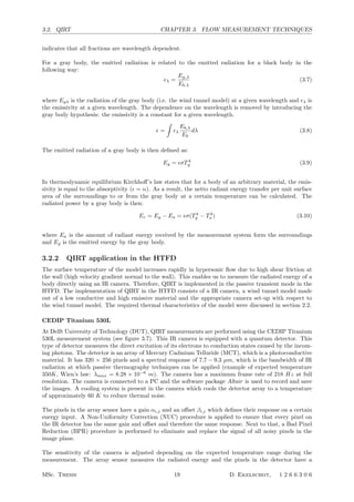
32. 3.1. SCHLIEREN PHOTOGRAPHY CHAPTER 3. FLOW MEASUREMENT TECHNIQUES
Figure 3.1: Graphical representation of Snell’s law
the other side, a similar parabolic mirror is located that directs the light to the camera. A knife edge is
located in the focal point of the mirror. This knife edge cuts off a portion of the light and it blocks the
bended light beams caused by density changes in the measurement plane. The set-up is shown in figure
3.2.
Figure 3.2: Set-up of the Schlieren system in the HTFD. Figure taken from Schrijer [2010a]
The physical principle of Schlieren visualisation is based on the fact that a local density change causes
a change in refractive index, as visualised in figure 3.3. The orange light ray that encountered a shock
wave, as shown in figure 3.3, is refracted downwards and therefore will appear in the image plane as a
dark line.
Figure 3.3: General working principle of Schlieren photography
MSc. Thesis 16 D. Ekelschot, 1 2 6 6 3 0 6

33. 3.2. QIRT CHAPTER 3. FLOW MEASUREMENT TECHNIQUES
3.1.3 Schlieren example
In figure 3.4, an example is given of a Schlieren image obtained during the current experiments. The knife
edge is aligned horizontally with the camera. From the principle explained in section 3.1.1 and 3.1.2, it
is determined that the shocks on the upper side of the model refract the light downwards and shocks
therefore appears as a black line. For the lower side of the model, the opposite is true. There, the shocks
refract the light upwards and they therefore appear as bright white lines. The model is placed in the test
section with the 45◦
ramp pointing downwards since the shock that emanates from the pitot tube in the
upper part of the test section impinges on the leading edge shock of the model. This is shown on the
lower side of the model in figure 3.4 since the image is flipped horizontally and vertically such that the
flow is from left to right.
Figure 3.4: Example of one of the obtained Schlieren images for the case of a zigzag VG with h = 1.15mm
and a Reunit = 14.1 × 106
m−1
.
3.2 Quantitative Infrared Theromography (QIRT)
Quantitative Infrared Thermography (QIRT) is often used to investigate the behaviour of the boundary
layer (transition, separation etc.) in hypersonic flow. This measurement technique is particularly inter-
esting for this flow regime since there is a clear interaction between the flow and the thermal state of the
surface. The surface temperature can be determined to obtain a qualitative description of the boundary
layer behaviour. However, the quantitative temperature is required when the surface heat transfer is
wanted. First, the basic infrared theory is discussed which is followed by a description of the measure-
ment system and set-up implementation in the HTFD. Finally, the data reduction technique is presented
which is used to obtain the surface heat flux.
3.2.1 Infrared theory
The emitted radiation energy of a body is directly related to the temperature of the body. Planck derived
an expression which relates the intensity radiated by a black body (perfect radiator) as a function of the
wavelength and surface temperature. Planck’s law is given by equation 3.3:
Eb,λ =
C1
λ5
e
C2
λTs − 1
(3.3)
C1 and C2 are constants. A black body is defined as a body that emits and absorbs at any temperature
the maximum possible amount of radiation at any given wavelength. The radiated energy by a black
body is plotted against the wavelength for a range of temperatures in figure 3.5.
MSc. Thesis 17 D. Ekelschot, 1 2 6 6 3 0 6

34. 3.2. QIRT CHAPTER 3. FLOW MEASUREMENT TECHNIQUES
10
−6
10
−5
10
7
10
8
10
9
10
10
λ [m]
Ebλ
[W
2
/µm]
T = 800 K T = 700 K
T = 600 K
T = 500 K
T = 400 K
T = 300 K
Figure 3.5: Planck’s law (blue lines) and Wien’s law (red line)
Note that the maxima (λmax) lie on a straight line in the logarithmic plane, which is referred to as Wien’s
law.
λmaxTs = 2.898 × 10−3
[m · K] (3.4)
The emitted radiation per unit surface area for a black body is then given by the Stefan-Boltzmann
equation:
Eb =
∞
0
Eb,λdλ =
qr
A
= σT4
s (3.5)
where A is the surface area, qr the heat transfer, Ts the surface temperature and the Stefan-Boltzmann
constant is given by σ = 5.67 × 10−8
W/(m2
K4
).
The wind tunnel model does not behave like a black body but is considered to be a so-called gray
body since it is not a perfect emitter. In general, a gray body absorbs a fraction (Iα), reflects a fraction
(Iρ) and transmits (Iτ ) a fraction of the incident radiation. The allocation of thermal energy after a body
is exposed to incident radiation is made clear in figure 3.6:
!
Figure 36 - Directional emissivity for non-
conductors
Figure 37 - Directional emissivity for conductors
When applying the gray-body hypothesis, the average emissivity for the wavelength band
where the bulk of radiation is emitted is used. Since this wavelength band changes with
temperature also the gray-body emissivity will change with surface temperature.
10.2.3Radiant thermal budget
Any object immersed in an environment exchanges energy with the surroundings through
radiation. The object receives energy by means of incident radiation . This incident radiation
can interact with the body in three ways.
Figure 38 - Radiant thermal budget
First a part of the energy is absorbed, absorption:
#$% ,
where is the absorption coefficient.
Secondly the radiation can be transferred through the object, transmission:
#'($) ,
where is the transmission coefficient.
Finally the incident radiation can be reflected, reflection:
#(*+, ,
where is the reflection coefficient.
Due to conservation of energy the incident radiation must either be reflected, transmitted or
absorbed resulting in the equality:
Figure 3.6: radiant thermal budget. Figure taken from Scarano [2007]
Mathematically this can be written as:
αλ + ρλ + τλ = 1 (3.6)
where αλ represents the absorbed fraction of the incident radiation, ρλ the reflected fraction of the inci-
dent radiation and τλ the transmitted fraction of the incident radiation [Scarano, 2007]. The subscript λ
MSc. Thesis 18 D. Ekelschot, 1 2 6 6 3 0 6

35. 3.2. QIRT CHAPTER 3. FLOW MEASUREMENT TECHNIQUES
indicates that all fractions are wavelength dependent.
For a gray body, the emitted radiation is related to the emitted radiation for a black body in the
following way:
λ =
Eg,λ
Eb,λ
(3.7)
where Egλ is the radiation of the gray body (i.e. the wind tunnel model) at a given wavelength and λ is
the emissivity at a given wavelength. The dependence on the wavelength is removed by introducing the
gray body hypothesis: the emissivity is a constant for a given wavelength.
=
λ
Eb,λ
Eb
dλ (3.8)
The emitted radiation of a gray body is then defined as:
Eg = σT 4
g (3.9)
In thermodynamic equilibrium Kirchhoff’s law states that for a body of an arbitrary material, the emis-
sivity is equal to the absorptivity ( = α). As a result, the netto radiant energy transfer per unit surface
area of the surroundings to or from the gray body at a certain temperature can be calculated. The
radiated power by a gray body is then:
Er = Eg − Ea = σ(T4
g − T4
a ) (3.10)
where Ea is the amount of radiant energy received by the measurement system form the surroundings
and Eg is the emitted energy by the gray body.
3.2.2 QIRT application in the HTFD
The surface temperature of the model increases rapidly in hypersonic flow due to high shear friction at
the wall (high velocity gradient normal to the wall). This enables us to measure the radiated energy of a
body directly using an IR camera. Therefore, QIRT is implemented in the passive transient mode in the
HTFD. The implementation of QIRT in the HTFD consists of a IR camera, a wind tunnel model made
out of a low conductive and high emissive material and the appropriate camera set-up with respect to
the wind tunnel model. The required thermal characteristics of the model were discussed in section 2.2.
CEDIP Titanium 530L
At Delft University of Technology (DUT), QIRT measurements are performed using the CEDIP Titanium
530L measurement system (see figure 3.7). This IR camera is equipped with a quantum detector. This
type of detector measures the direct excitation of its electrons to conduction states caused by the incom-
ing photons. The detector is an array of Mercury Cadmium Telluride (MCT), which is a photoconductive
material. It has 320 × 256 pixels and a spectral response of 7.7 − 9.3 µm, which is the bandwidth of IR
radiation at which passive thermography techniques can be applied (example of expected temperature
350K, Wien’s law: λmax = 8.28 × 10−6
m). The camera has a maximum frame rate of 218 Hz at full
resolution. The camera is connected to a PC and the software package Altair is used to record and save
the images. A cooling system is present in the camera which cools the detector array to a temperature
of approximately 60 K to reduce thermal noise.
The pixels in the array sensor have a gain αi,j and an offset βi,j which defines their response on a certain
energy input. A Non-Uniformity Correction (NUC) procedure is applied to ensure that every pixel on
the IR detector has the same gain and offset and therefore the same response. Next to that, a Bad Pixel
Reduction (BPR) procedure is performed to eliminate and replace the signal of all noisy pixels in the
image plane.
The sensitivity of the camera is adjusted depending on the expected temperature range during the
measurement. The array sensor measures the radiated energy and the pixels in the detector have a
MSc. Thesis 19 D. Ekelschot, 1 2 6 6 3 0 6

36. 3.2. QIRT CHAPTER 3. FLOW MEASUREMENT TECHNIQUES
Figure 3.7: The CEDIP camera
saturation level. The sensitivity of the detector is therefore determined by the exposure time. For a
temperature range of 323K ≤ T ≤ 473K, an exposure/integration time of τ = 72µs is used while for a
lower temperature range, 253K ≤ T ≤ 323K, the integration time is increased to τ = 340µs. For both
integration times, a calibration function is available so that the energy levels measured by the camera
are transformed into temperature levels. Both integration times are used since the model tested in the
current experiments, consists of two ramps and each ramp is exposed to a different range of temperature.
For this reason, two FOVs are determined which are given in figure 3.8. For both FOVs the domain of
interest is highlighted by the red lines.
(a) The FOV when the surface temperature is mea-
sured of the 5◦ ramp (θ1 = 5◦) with τ = 340µs
(b) The FOV when the surface temperature is mea-
sured of the 45◦ ramp (θ2 = 45◦) with τ = 72µs
Figure 3.8: The two FOVs for the test case hzz = 1.15 mm and Reunit = 14.1 × 106
[m−1
]
The expected temperature range on the 5◦
ramp lies below 320 K. The integration time is therefore set
to 340 µs to increase the sensitivity of the camera. For the 45◦
ramp holds that the expected temperature
range lies beyond 320 K, hence, the integration time of the sensor is set to 72 µs. Note the occurrence of
pixel saturation in the FOV with the 5◦
ramp in focus (see figure 3.8(a)). On the left hand side a small
part of the 45◦
ramp can be seen. The uniform dark red colour indicates that the maximum energy level
of the pixel is reached due to the long integration time. In figure 3.8(b), the integration time is set to
τ = 72 µs since for this (lower) integration time, no pixel saturation occurs at the second ramp.
Measurement set-up
An optical window does not have a sufficient transmissivity for the IR camera to register the temperature
at a surface within the test section. Therefore, a Germanium window is fitted in the test section of the
HTFD since Germanium has a transmissivity of approximately 0.8 [Schrijer, 2010b]. This is indicated in
figure 3.9(a).
As mentioned before, the sensor of the camera is cooled to reduce thermal noise. Hence, self reflec-
tion occurs whenever the camera is placed normal with respect to the test section window. Therefore,
the camera is set under an angle with respect to the normal of the test section window (see figure 3.9(a)).
The emissivity changes with the optical angle θ which is the angle between the surface normal and the
MSc. Thesis 20 D. Ekelschot, 1 2 6 6 3 0 6

37. 3.2. QIRT CHAPTER 3. FLOW MEASUREMENT TECHNIQUES
(a) The camera set-up with respect to the test section and
the model during a QIRT experiment. Image taken from
Schrijer [2010a]
= λ
Eb,λ
Eb
dλ (4.6)
Finally Kirchhoff’s law states that the spectral emissivity is equal to the spectral
absorptivity for any specified temperature and wavelength, λ = αλ.
Since a gray body has a constant spectral emissivity, its total emitted radiation can
Figure 4.2: Gray body radiator [49]
Figure 4.3: Variation of directional
emissivity for several electrical noncon-
ductors [49]
be related to the total radiation emitted by a black body using the Stefan-Boltzmann
equation (4.3)
Eo = σT4
s . (4.7)
55
(b) The variation in directional emissivity for several elec-
trical nonconductors
Figure 3.9: The camera set-up with respect to the test section and the model during a QIRT experiment
and the variation in directional emissivity for several electrical nonconductors [Scarano, 2007]
direction of the radiant beam emitted from the surface of the model. Based on the polar plot given
in figure 3.9(b), the directional emissivity is taken to be constant for optical angles smaller than 50◦
.
Therefore, the viewing angle of the camera with respect to the radiating surface, cannot exceed 50◦
.
3.2.3 Data reduction technique
While recording, the tunnel is fired and a short movie of 3 seconds is recorded using Altair. A typical
data set consists of approximately 20 frames since the acquisition frequency of the camera is set to 218
Hz and the measurement time is approximately 120 ms. The data acquired with the CEDIP IR camera
is saved in .ptw format which is read into Matlab. The pixel energy level at a fixed point in the image
plane is plotted against the measurement time and a typical profile is shown in figure 3.10.
400 500 600 700 800 900 1000 1100 1200 1300
2200
2300
2400
2500
2600
2700
2800
t [ms]
E
meas
[W/m
2
]
End of the run
Start of the run
Figure 3.10: The measured data at a local point in the measurement plane (xpix, ypix) = (150, 150)
Note the small jump at t = 800 ms which indicates the start of the run. The starting point is located
by setting a threshold on the gradient of the signal. Based on the starting point, a range of images is
MSc. Thesis 21 D. Ekelschot, 1 2 6 6 3 0 6

38. 3.2. QIRT CHAPTER 3. FLOW MEASUREMENT TECHNIQUES
taken such that the start and the end of the measurement are subtracted from the large data set. The
average heat transfer distribution is calculated using 15 images during the run. The energy jump at the
end of the run is caused when the valve of the wind tunnel is closed and the model is still present in the
low speed hot gas flow. After that, the gradual cooling of the gas takes place, indicated by a decrease in
energy level from t = 1000 ms. A run time of approximately 120 ms is determined when observing the
energy profile at a single point in the image plane (see figure 3.10).
The quantitative temperature is acquired using a conversion function that is obtained during the calibra-
tion procedure for the IR camera. The 1D semi infinite heat equation is solved to determine the heat flux
at the wall. This is a inverse problem since the surface temperature is measured and one of the boundary
conditions −k ∂T (0,t)
∂y = qs(t) is unknown. Schultz and Jones [1973] obtained the following solution:
qs(t) =
ρck
π
t
0
dTs(τ)
dτ
√
t − τ
dτ (3.11)
This is a rather inconvenient expression to work with since it requires the temperature gradient. Therefore
a cumulative heat input, Q(t), is taken instead of the instantaneous convective heat flux, qs.
Q(t) =
t
0
qs(τ)dτ =
ρck
π
t
0
Ts(τ)
√
t − τ
dτ (3.12)
Equation 3.12 is numerically integrated by taking φ(τ) = T(t)−T(0). Cook and Felderman approximated
φ(τ) by a linear function:
˜φ(τ) = φ(ti−1) +
φ(ti) − φ(ti−1)
∆t
(τ − ti−1) (3.13)
where ti−1 ≤ τ ≤ ti and i = 1, 2, 3, ..., n and determined this directly into equation 3.12:
Q(tn) =
ρck
π
n
i=1
φ(ti−1) + φ(ti)
√
tn − ti−1 +
√
tn − ti
dt (3.14)
using a finite difference scheme, equation 3.14 is numerically implemented in the following way:
qs(tn) =
Q(tn)
dtn
=
−2Q(tn−8) − Q(tn−4) + Q(tn+4) + Q(tn+8)
40(tn − tn−1)
(3.15)
The quantity of interest during the QIRT measurement campaign is the surface heat flux, which is given
in W/m2
. This is non dimensionalised by dividing the surface heat flux by the enthalpy potential at the
wall, the density and the velocity. The Stanton number is defined in equation 3.16.
St =
qs
ρeUe(haw − hw)
(3.16)
where ρe and Ue are the density and the streamwise velocity at the edge of the boundary layer, respectively.
The enthalpy for the adiabatic wall is indicated by haw and the wall enthalphy is indicated by hw. The
Stanton number relates the convective surface heat transfer to the convected enthalpy in the free stream
and this is often determined when dealing with a short duration measurement. Because the density
and the streamwise velocity at the edge of the boundary layer are not available and the adiabatic wall
temperature in a short duration measurement facility cannot be determined accurately, a slightly modified
version of the Stanton number is used:
ch =
qs
cpρ∞u∞(Tt − Tw)
(3.17)
where Tt is the total temperature and Tw the wall temperature. The free stream density and free stream
velocity are easily determined and it is assumed that the gas is calorically perfect so that h = cpT.
MSc. Thesis 22 D. Ekelschot, 1 2 6 6 3 0 6

39. 3.3. PIV CHAPTER 3. FLOW MEASUREMENT TECHNIQUES
3.3 Particle Image Velocimetry (PIV)
Particle Image Velocimetry (PIV) is a non-intrusive flow measurement technique, which is based on the
direct measurement of particle displacement in a planar field by means of image cross correlation. A
plane is illuminated by laser light and tracer particles are introduced in the flow. The camera records
the particle distribution in the Field Of View (FOV) at two time instants. By means of image cross
correlation, the velocity field is obtained. A typical PIV measurement consists of following steps.
Step 1: Determine the Field Of View (FOV)
Step 2: Align the laser sheet with the FOV
Step 3: Align the calibration plate with the laser sheet
Step 4: Introduce tracer particles in the flow
Step 5: Double pulsed laser illuminates the tracer particles with laser light
Step 6: Record the particle distribution at t1 = t0 and t2 = t0 + ∆t
Step 7: Image processing using 2D-cross correlation to determine the velocity field
Data storage
and processing
Seeded Flow
Laser light sheet
Illuminated
particles
CCD camera
To image acquisition system
Figure 3.1: Configuration of a PIV experiment
ing principle with particular attention to the critical aspects of PIV measurements in
hypersonic flows.
3.2.1 Flow seeding
The selection of a suitable particle type is an assessment of light scattering capability,
particle response and handling characteristics which dictate conflicting requirements.
The light scattering capability of a particle is determined by the ratio of the particle
refractive index to the surrounding refractive index, the particle size, shape and ori-
entation. Furthermore also the polarization and observation angles have an important
influence [63]. When the particle size is larger than the wavelength of the incident
light λ, Mie scattering occurs. When the particle size is smaller than λ, Rayleigh
scattering occurs. For Mie scattering the average intensity increases with d2
p where
dp is the particle diameter, in case of Rayleigh scattering the intensity varies with
d6
p. From this it becomes evident that the particle scattering capability decreases
strongly with the particle diameter, especially when the particles become so small
that Rayleigh scattering occurs. So within the limits between Mie and Rayleigh scat-
tering a particle diameters as large as possible is desired.
This however contrasts with the requirement that a particle has to faithfully follow
the flow. This is especially important in high speed flow where large accelerations
occur (e.g. shock waves and expansion waves). The particle fidelity can be quantified
through the relaxation time τ (see section 3.3.1):
τ =
4ρpd2
p
3cdRedµf
(3.1)
where ρp is the particle density, cd is the particle drag coefficient, Red is the particle
Reynolds number and µf is the flow viscosity. When the relaxation time is high, the
particle fidelity is low. This shows that in order to minimize the relaxation time, the
Figure 3.11: Schematic representation of the working principle of a 2C-PIV experiment. Figure taken
from Schrijer [2010a]
The tracer particles, particle illumination and imaging and the image processing are discussed in the
coming sub-sections.
3.3.1 The tracer particles
The tracer particles are directly introduced in the hot storage tube by means of a cyclone seeder. This
is a cylindrical vessel with a tube inside through which air is blown against the side of the vessel. In this
way a cyclone is created which is driven by the pressure difference between the hot storage tube and the
reservoir tanks. The lightest particles are then located in the upper part of the vessel. The particles are
driven into the hot storage tube by opening the valve between the cyclone seeder and the storage tube.
The cyclone seeder implemented in the HTFD together with a visualisation of the working principle is
shown in figure 3.12.
Because of the high temperature conditions present in the storage tube, the thermal properties have to
be taken into account while choosing for the appropriate material of the tracer particle. Titanium dioxide
(TiO2) tracer particles are used during PIV measurements in the HTFD since these particles can easily
withstand heating up to 800 K in the HTFD storage tube, follow the flow smoothly and they have good
light scattering properties.
The tracer particles encounter high velocity gradients (shocks) when PIV is applied in compressible
MSc. Thesis 23 D. Ekelschot, 1 2 6 6 3 0 6

40. 3.3. PIV CHAPTER 3. FLOW MEASUREMENT TECHNIQUES
e particles used for measurements in the HTFD are composed of titanium-dioxide (TiO2, Kemira UV-TITAN
0) with a nominal crystal size of 50 nm and a nominal bulk density of ρb = 200 kg/m3
. The seeding is
ed to the the fluid stored in the pressure tube prior to the wind tunnel run by means of a high pressure
lone. A pressure difference is applied between the storage tube of the HTFD and the cyclone, allowing to
nsport seeded fluid into the storage tube. Figure 3.4 shows the cyclone next to the storage tube.
Figure 3.4: Cyclone seeding device(a) Cyclone seeder at the HTFD. Image taken from
Caljouw [2007]
A Melling
Figure 8. A cyclone aerosol generator.
by dilution in the flow. Aggregation tends to increase as the
flow through the bed is increased, so that the bed density
becomes non-uniform and is disturbed by bubbles or slugs
of air, leading to an erratic rate of generation.
To improve the stability of the particle generation
from a fluidized bed, Glass and Kennedy (1977) used an
additional cyclone to obtain 0.1–1 µm Al2O3 particles
(figure 8). For particle concentrations above 109
m−3
,
concentration fluctuations were greatly reduced. This
generator design was adopted for PIV experiments, for
example, by Anderson et al (1996).
In an effort to obtain steadier distributions of
concentration and particle size than is possible with
conventional fluidized beds, two-phase beds have been
developed (Willeke et al 1974, Guichard 1976). The
bed (figure 9) contains a mixture of beads (nickel, bronze
or glass, diameter 100–200 µm) and the powder to be
dispersed. The suspended powder particles are much
smaller than the beads and can move freely in the
volume between the beads without forming gas bubbles.
The continuous friction between the beads reduces the
aggregation of the powder particles. The upwards gas
velocity is set between the gravitational settling velocities
of the particles and the beads, so that the beads are fluidized
but not entrained. The powder particles are elutriated from
the bed by rising gas bubbles which burst at the surface of
the bed, releasing the particles. A generator of essentially
this type was previously offered commercially for LDA
and PIV experiments by TSI Inc, St Paul, USA, but is
now no longer in production. The design and operating
characteristics of such a generator, although it was not
intended for PIV experiments, were described by Boucher
and Lua (1982).
The simple fluidized bed or variants thereof has
been found to be more practical than, for example, the
complicated spark discharge generator described by Altgeld
et al (1980). An ultrasonic disperser is another means of
introducing larger seeding particles into an air stream and
has been used by Schmidt and L¨offler (1993) with 30 µm
glass particles for PIV experiments.
Figure 9. A ‘
5.2. The seeding of sca
5.2.1. Seeding in liqu
in liquid flows are alm
circuit test loops. It is,
concentrated suspension
before starting the mea
to mix thoroughly and
Dilutions up to 1:50 0
monodisperse suspensio
be used, but these are m
large quantities.
5.2.2. Seeding in gas
be introduced into th
concentration, with a sp
minimizing coagulation
windows. Frequently
global and local seeding
Global seeding, wit
flow well upstream of
preferable to ensure tha
region, so that velociti
PIV experiment are rep
a spatially homogeneou
seeding concentration in
et al (1992) introduced
section and allowed them
Possibilities for varyin
closed-circuit tunnel inc
intermittently or allowi
switching off the genera
to a level suitable for P
are, of course, only fe
seeding concentration ex
wind tunnels seeding the
of the limited productio
If only a restricted
interest, it may be accep
passing through the obs
1414
(b) Working principle of the cyclone seeder. Image
taken from Melling [1997]
Figure 3.12: Cyclone seeder.
flow. A tracer particle needs a specific amount of time to adjust to the local surrounding velocity when-
ever it passes through a shock which is defined as the particle response time. The response time is highly
dependent on the particle diameter and it plays therefore a significant role when selecting the tracer par-
ticle for PIV in compressible flow. Considering the simplified equation of motion of a spherical particle
in air [Melling, 1997].
πd3
p
6
ρp
dup
dt
= −3πµdp (u − up) →
∂up
∂t
=
u − up
τp
(3.18)
up and u represent the particle velocity and the local flow velocity respectively. Furthermore, ρp represents
the particle density, µ the viscosity coefficient, dp the particle diameter. The particle response time is
indicated by τp where τp is defined as:
τp =
d2
pρp
18µ
(3.19)
The response time is generally modeled as a exponential function of time when a shock is present. To
determine the response time of the particle crossing a shock wave, the following relation is used:
e
− t
τp =
un,p − un,1
un,2 − un,1
(3.20)
where u is the velocity of the particle, un,1 the normal velocity of the flow in front of the shock and un,2
the normal velocity behind the shock. The particle velocity and fluid velocity are plotted against t
τ in
figure 3.13.
It can be seen from figure 3.13 a small particle diameter or low density, results in a short response time
which is wanted during PIV measurements in short duration test facilities.
A spatial displacement is measured with PIV and therefore it is interesting what consequences are at-
tached to the response time in terms of spatial behaviour of the particle. Therefore, equation 3.20 is
rewritten in terms of up:
up = e
tp
τ (u1 − u0) + u1 (3.21)
Equation 3.21 can be integrated to determine xp which represents the particle displacement with respect
to the velocity discontinuity (shock):
tp
0
updt = xp =
tp
0
e
tp
τ (u1 − u0) + u1dt = −τe
tp
τ (u1 − u0) + u1τ + ˜C (3.22)
MSc. Thesis 24 D. Ekelschot, 1 2 6 6 3 0 6

41. 3.3. PIV CHAPTER 3. FLOW MEASUREMENT TECHNIQUES
−2 0 2 4 6 8
0
0.2
0.4
0.6
0.8
1
t/τ
u
*
=(up
−u2
)/(u1
−u2
)
Particle velocity d = d
0
Particle velocity d = 1.41 d0
Particle velocity d = 1.73 d
0
Fluid velocity
∆U/e
Figure 3.13: Particle velocity plotted together with the velocity of the fluid passing through a shock
Taking the initial condition (x0, t0) = (0, 0) and substituting tp = τ ln
up−u1
u1−u0
into equation 3.22 results
in:
xp = u1τ ln
u0 − u1
up − u1
+ τ (u0 − up) (3.23)
It is assumed that the term (uu − up) is small compared to the first right hand side term and therefore,
the particle response time can be written in terms of the particle displacement:
u∗
= e
−xp
ξ (3.24)
where xi is the relaxation length which is related to the response time using equation 3.23:
ξ = τ
u0 − (u0 − u1)e−1
(3.25)
It is then concluded that for larger particle sizes, the response time and thus the relaxation length
increases. The choice for 50 nm TiO2 tracer particle is therefore based on a trade-off between short
response time and proper scattering characteristics. The eventual particle size is 400 − 500 nm due to
particle agglomeration. A scanning electron microscopy image of the 50 nm TiO2 particles is given for
both single particles and a agglomeration of particles in figure 3.14.
PIV’05
3
PIV MEASUREMENT SYSTEM
Flow seeding
Titanium dioxide (TiO2) particles with a nominal crystal size of 50 nm are used (Kemira UV-TITAN L830) with a
bulk density of !b = 200 kg/m3
. Figure 1 shows an electron scan of the particles kindly provided by Kronos
International, (Leverkusen, DE). From the qualitative inspection of the picture it may be concluded that the nominal
crystal size is indeed about 50 nm (a particle is about one tenth of the line that is equal to 500 nm). However as can
be seen from -right, the particles tend to cluster to a nominal size of approximately 200 nm. The quantitative analysis
of the sample returns a median particle diameter of 376 nm with a dispersion of 200 nm.
Figure 1 – Electron microscopy images of TiO2 particles. Left: image of a collection of particle agglomerates; right a
single agglomerate.
The seeding particles are introduced in the hot storage tube off-line by means of a high-pressure cyclone device.
The inlet is placed in proximity of the valve (Figure 2). The amount of seeding introduced in the storage tube
requires a careful control, which is achieved introducing the seeded air flow by a finite amount through successive
charge-discharge of the seeder chamber fluid into the hot storage tube. However the method does not ensure a
uniform distribution of the seeding particles along the storage tube where the seeding particles are transported by the
inflow and mixed by some thermal convection. Therefore the seeding density level will also vary (decrease in this
case) during the run time of the tunnel. The current hardware allows a maximum measurement frequency of 10 Hz,
where only one snapshot can be acquired during a run. The seeding level is therefore optimized for a given time
instant (40 ms after the valve opening) selected for the measurement. An optimum delay is experimentally
determined, enabling the current system to produce well-controlled and repeatable seeding conditions.
(a) Electron scan of TiO2 particles which
shows an indication of the diameter of a
single TiO2 particle (50 nm)
PIV’05
3
PIV MEASUREMENT SYSTEM
Flow seeding
Titanium dioxide (TiO2) particles with a nominal crystal size of 50 nm are used (Kemira UV-TITAN L830) with a
bulk density of !b = 200 kg/m3
. Figure 1 shows an electron scan of the particles kindly provided by Kronos
International, (Leverkusen, DE). From the qualitative inspection of the picture it may be concluded that the nominal
crystal size is indeed about 50 nm (a particle is about one tenth of the line that is equal to 500 nm). However as can
be seen from -right, the particles tend to cluster to a nominal size of approximately 200 nm. The quantitative analysis
of the sample returns a median particle diameter of 376 nm with a dispersion of 200 nm.
Figure 1 – Electron microscopy images of TiO2 particles. Left: image of a collection of particle agglomerates; right a
single agglomerate.
The seeding particles are introduced in the hot storage tube off-line by means of a high-pressure cyclone device.
The inlet is placed in proximity of the valve (Figure 2). The amount of seeding introduced in the storage tube
requires a careful control, which is achieved introducing the seeded air flow by a finite amount through successive
charge-discharge of the seeder chamber fluid into the hot storage tube. However the method does not ensure a
uniform distribution of the seeding particles along the storage tube where the seeding particles are transported by the
inflow and mixed by some thermal convection. Therefore the seeding density level will also vary (decrease in this
case) during the run time of the tunnel. The current hardware allows a maximum measurement frequency of 10 Hz,
where only one snapshot can be acquired during a run. The seeding level is therefore optimized for a given time
instant (40 ms after the valve opening) selected for the measurement. An optimum delay is experimentally
determined, enabling the current system to produce well-controlled and repeatable seeding conditions.
(b) Agglomeration of TiO2 particles with
an approximate mean diameter of 376 nm
Figure 3.14: Scanning Electron Microscope (SEM) images of the TiO2 50 nm particle tracers. Figures
taken from Schrijer et al. [2005]
3.3.2 Particle imaging and illumination
A Quanta-Ray double-cavity Nd:YAG laser from Spectra-Physics is used to illuminate the particles. This
device generates light pulses at a wavelength of 532 nm with a maximum energy of 400 mJ per pulse
and a duration of 6 ns. The Quanta-Ray double-cavity Nd:YAG laser is located below the test section.
MSc. Thesis 25 D. Ekelschot, 1 2 6 6 3 0 6

42. 3.3. PIV CHAPTER 3. FLOW MEASUREMENT TECHNIQUES
In figure 3.15, a sketch of the laser set-up underneath the test section is shown.
Figure 3.15: The laser set-up
The laser head creates a green bundle of laser light which has a wavelength of λ = 532nm. The first
plano concave lens that the laser beam encounters, widens the beam in one direction. The plano convex
lens is rotated with respect to the plano concave lens to widen the beam in the other direction. Hence,
the thickness of the beam is increased by a combination of a plano-concave and convex lenses. A mirror
points the optically widened laser beam upwards where the beam meets again a plano-concave lens which
creates the wide sheet. The thickness of the laser sheet is controlled by changing the distance between
the first plano-concave lens and plano-convex lens (L) below the test section.
The images are recorded using a 1376 × 1040 pixel SensiCam Quantum Efficiency (QE) camera. This
type of camera records with a minimum separation time of 0.5 µs and has a high sensitivity. The size of
the pixel is 6.45 × 6.45 µm2
. This type of camera has a maximum frame rate of 10 Hz and therefore one
image is recorded during the measurement time of 120 ms. The camera and the laser are synchronised
with the wind tunnel so that at 30 ms from the start of the run, a measurement is taken. The images
are recorded using Lavision Davis 7.4.
The magnification is determined by placing a Lavision Type 10 calibration plate with equally spaced
dots in the Field Of View (FOV). The distance between the dots is 10 mm. A magnification factor is
found using the imtool in Matlab:
M =
ddot
dpix
=
0.01m
273.39pix
= 3.66 × 10−5
m/pix (3.26)
where ddot is the spacing between the dots on the calibration plate and dpix is the measured length in
pixels on the image plane obtained using Matlab. Based on the magnification factor and the expected
velocity magnitude, u, the separation time between the two captured frames (∆t) is determined:
∆pix =
u
M
· ∆t → ∆t =
M∆pix
u
=
3.66 × 10−5
· 20
1000
= 730ns (3.27)
where∆ pixx is the wanted pixel displacement which is based on the one-quarter rule for the in-plane
particle image displacement. Due to an inaccurate synchronisation of the camera and the laser, the
separation time is set to∆ t = 1µs for 2C-PIV measurements performed during this thesis project. The
recording system captures the scattered light from the particles in the flow. The image particle diameter
is dependent on the magnification, the particle diameter and the diffraction spot diameter:
dτ =
(Mdp)2 + d2
d (3.28)
MSc. Thesis 26 D. Ekelschot, 1 2 6 6 3 0 6

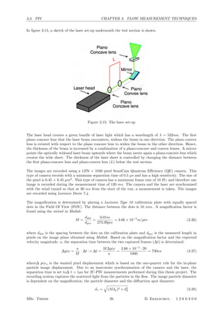
43. 3.3. PIV CHAPTER 3. FLOW MEASUREMENT TECHNIQUES
where the diffration spot diameter is determined by:
dd = 2.44f#(M + 1)λ (3.29)
where f# is the ratio between the focal length and the aperture of the camera. The aperture of the
camera is adjusted such that no particle streaking is present and a particle image of approximately 2
pixels is obtained.
3.3.3 Image processing
The recorded images are processed using Lavision Davis 7.4 using a 2D-cross correlation procedure.
Initially the background is extracted using a non-linear sliding minimum filtering which is a build in
function in Lavision Davis 7.4. The particles in the second image are displaced with respect to the first
image and therefore, 2D cross correlation is suitable to obtain the particle displacement. The image at
t1 = t is referred to as image A and the image at t2 = t + ∆t is referred to as image B. Both image
A and B are split up into interrogation windows which represent the local particle intensity map. The
interrogation window in image A is cross correlated with the corresponding interrogation window in image
B. As a result, a local peak is found in the correlation map. The displacement in x and y of the peak
with respect to the center of the correlation map represents the mean local particle displacement within
the interrogation window. This is shown in figure 3.16.
Figure 3.16: 2D cross correlation procedure
The particle intensity images are represented by Ea(x, y) and IB(x, y) for each interrogation window.
The cross correlation consists of the convolution of the Ea(x, y)− ¯IA with IB(x+∆x, y +∆y)− ¯IB which
is then divided by the corresponding standard deviation:
R(∆x, ∆y) =
xwx,ywy
x=1,y=1
(Ea(x, y) − ¯IA)IB(x + ∆x, y + ∆y) − ¯IB)
xwx,ywy
x=1,y=1
(Ea(x, y) − ¯IA)2
xwx,ywy
x=1,y=1
(IB(x + ∆x, y + ∆y) − ¯IB)2
(3.30)
where wx and wy are the size of the interrogation window in x and y given in pixels. From R(∆x, ∆y)
the peak is determined and the velocity vector is calculated based on the peak displacement with respect
to (0, 0) in the correlation map.
u = M
∆x
∆t
(3.31)
where M is the magnification,∆ u = [ ∆u, ∆v]T
and∆ x = [ ∆x∆y]T
. This procedure is applied for every
interrogation window such that the local velocity vector is determined in the complete measurement
MSc. Thesis 27 D. Ekelschot, 1 2 6 6 3 0 6

44. 3.3. PIV CHAPTER 3. FLOW MEASUREMENT TECHNIQUES
domain.
The spatial resolution is increased by decreasing the interrogation window size using a multi-iterative
correlation procedure. Initially, a large interrogation window is chosen to ensure the one-quarter rule for
the in-plane particle image displacement. A typical final window size is 32 × 32 pixels with 75% overlap.
Based on the obtained magnification factor, the spatial resolution is given in table 3.1.
Table 3.1: Number of vectors in x and y direction during the performed 2C-PIV measurements in the
HTFD
x y
vec/mm 3.78 3.71
Typically it is wanted to have at least 9 particle pairs within the interrogation window since the height of
the correlation peak (S/N) is directly dependent on the amount of particle pairs. This argument follows
directly from the definition of cross correlation. For a uniform particle distribution, the amount of pixels
in the interrogation window is determined using equation 3.32.
Ntot =
ppp
9
(3.32)
where ppp is Particle Per Pixel. For a square interrogation window, the window size is determined
by N =
√
Ntot. However, there are particle density gradients present in the images since the flow is
compressible and particle slip occurs [Schrijer, 2010a, Elsinga, 2008] (see section 3.3.1). The shape of
the interrogation window is adjusted such that the spatial resolution is increased in a particular region
and/or direction as long as the total amount of pixels per interrogation window fulfills equation 3.32.
particle displacement as:
v = M
∆x
∆t
(3.5)
where M is the magnification and ∆t is the laser pulse time separation. Subsequently
a second interrogation region is selected and the process is repeated. This is done
until the complete image is analyzed.
Figure 3.5: Two superimposed exposures
within an interrogation window. First ex-
posure is red and second exposure is green
! x! y
R(!x,!y) Figure 3.6: Correlation map
In order to improve accuracy and robustness an iterative approach is used. First,
a multi-grid analysis is applied where the interrogation window size is progressively
decreased [85]. This process eliminates the 1
4 rule constraint [63] and it is usually
terminated when the final window size is reached. Hereafter iterative analysis is
performed at a fixed sampling rate (grid spacing) and window size. This process
allows to further improve the accuracy of the image deformation ([70]; [60]; [87]) and
to a certain extent allows to enhance the spatial resolution of the measurement [74].
Furthermore in the iterative loop image deformation (see figure 3.7) is applied in order
to minimize errors due to in-plane velocity gradients.
Iterative image deformation methods in
x
y
(b)
(b')
d
(b’)
(a’)
Interrogation. location
d
Figure 8. Window shift method with FDI (left) and with CDI (right). Piecewise uniform displacement predictor distribution.
x
y
x
y
(a)
d
t0 t0+ t∆
(b')(b)
Figure 9. Schematic illustration of the image transformation due to
linear in-plane motion. Particles follow the mean displacement d
(translation) and the local displacement gradient.
crucial aspect in such a procedure and it must be consistent
with signal theory. Suitable schemes must be adopted so
as to avoid or minimize image degradation or signal loss
(Niblack 1986). Common choices are multidimensional
polinomial interpolation (bilinear biquadratic, bicubic splines)
and regression formulae such as least-squares biquadratic.
3.1.2. Linear displacement predictor. When the
displacement distribution is obtained after a first image
interrogation, the continuous displacement distribution
(piecewise linear) can be estimated using a two-dimensional
linear interpolation with respect to the interrogation grid points
(figure 9).
Huang et al (1993b) contributed to the development
of such an approach, proposing the particle pattern image
distortion (PID) technique. The major goal of the
technique was that of maximizing the effective particle
image pattern (PIP) matching during the cross-correlation
analysis. As a result, the technique brought a significant
improvement, enlarging the vorticity dynamic range with
respect to conventional cross-correlation. The work is widely
referred to in subsequent literature studies that followed similar
approaches. The authors showed that the distortion of the
interrogation window allowed the measurement of the particle
image displacement over a larger range of the velocity gradient
with respect to the traditional correlation. The maximum
velocity gradient measured was 55.3 s−1
(1.1 pixel/pixel
deformation rate) compared with 15 s−1
(0.5 pixel/pixel) from
Willert and Gharib (1991). However, the analysis of synthetic
images of a simulated Oseen vortex yielded a measurement
PIP method are reported in figure 10. Clearly it is possi
to enlarge the range of the measurable velocity gradient. T
effectiveness of the image distortion procedure is proven
the higher S/N level (consequently a lower yield of spuri
vectors) in the highly sheared/vortical region downstream
the separation point. In comparison, the conventional cro
correlation for a given choice of the S/N threshold fails in
region of higher vorticity.
However, the method was implemented with a h
computational cost since there was a high resolution associa
with the dense data spacing obtained by means of a la
overlap between adjacent windows.
Moreover, a relatively simple image reconstruct
scheme (bilinear interpolation) and the sub-pixel correlat
peak fit (centroid) are considered inaccurate for the im
resampling and for the correlation peak location estim
as was demonstrated in later studies (Westerweel 19
Louren¸co 1996). Therefore, the above implementation
not completely succeed in exploiting the benefit of the im
deformation philosophy in terms of measurement precision
A method similar to PID was proposed by Jambunath
et al (1995) who also evaluated the method’s performance
means of synthetic PIV images with a known particle im
displacement.
The choice of the displacement distribution to test
method performance was made on the basis of physi
considerations; namely, the Helmoltz velocity theory w
invoked that divides the movement of a fluid element into th
subsidiary terms:
V (r) = V0 + 1
2
V δr + φ (3
where V (r) is the velocity distribution across the fluid eleme
The three terms in the right-hand side of the equation
translation, rotation and bi-axial shear, respectively.
The two most important outcomes were that (a)
measurement accuracy can be improved from a factor of 2
5 using the image deformation method and (b) the correlat
peak height is weakly dependent of the in-plane displacem
distribution.
The assessment of the method returned a measurem
error level of only 0.02 pixels on synthetic particle ima
Figure 3.7: Image deformation according to the local velocity field, taken from [70]
The iterative equation of the PIV process can be described as:
V k+1
= V k
+ Ck+1
(3.6)
Where V k
indicates the result of the evaluation at the kth
iteration and is used as
predictor for the following iteration. The correction term Ck
= (cu, cv) is the vector
42
Figure 3.17: graphical representation of window deformation
By means of window deformation, a higher spatial resolution is achieved while maintaining a sufficient
S/N. The velocity vector which is obtained after the first iteration is used as a initial predictor. Using a
iterative correlation procedure, the interrogation window A and B are deformed based on the previously
determined velocity field in the following way [Scarano, 2002].
IA,new = Ea(x +
up∆t
2
, y +
vp∆t
2
)
IB,new = IB(x + ∆x −
up∆t
2
, y + ∆y −
vp∆t
2
)
where up and vp are the local velocity at a pixel. The velocity vector at every pixel location is determined
using bilinear interpolation and the window is deformed as shown in figure 3.17. The iterative window
deformation procedure is presented by the block diagram given in figure 3.18:
The velocity vector is then updated accordingly:
vnew = v + Cnew (3.33)
where Cnew is the corrector and defined as Cnew = IA,new ⊗ IB,new.
MSc. Thesis 28 D. Ekelschot, 1 2 6 6 3 0 6

45. 3.4. TOMO-PIV CHAPTER 3. FLOW MEASUREMENT TECHNIQUES
2 2
Ik
b (x, y) = Ib
x +
uk
d
2 , y +
vk
d
2
(3.7)
Here (ud, vd) is the image deformation displacement at location (x, y) commonly ob-
tained interpolating the predictor displacement V k
onto a pixel grid. The whole image
interrogation process is described schematically in figure 3.8.
select windows
convergence
Vd
k
build deformation
field
update result
predictor + corrector
k+1
V
a bII
deform images
k k
cross correlation
C
k+1
I Iba
read images
Figure 3.8: Block diagram of the iterative image deformation interrogation method
The most common choice for the displacement interpolation is bi-linear ([41], [43],
[70]) which is also used in the current applications. Higher order functions have also
been considered ([33]; [50]), which may in principle improve the accuracy of image
deformation. In all cases where a sub-pixel image transformation is performed (sub-
pixel window shift and window deformation), the images have to be interpolated for
re-sampling at non-integer pixel positions. The topic is extensively discussed by As-
tarita [7], who concluded that high-order interpolators are necessary to achieve higher
accuracy. However, high noise levels may reduce the relative improvements obtained
for high order interpolators [6]. In the current applications image interpolation is
performed using a sinc interpolation with a 11 × 11 pixel kernel size.
Furthermore filtering is applied in order to prevent the iterative process to become
unstable [74]. This is done by applying a two-dimensional second order regression
filter to the displacement field. It has been shown that this filter has a favorable
combination of noise reduction behavior and low spatial modulation.
3.2.4 Stereoscopic PIV
Stereoscopic PIV is used in order to obtain the three component velocity vector field
in the measurement plane. As the name indicates, the measurement principle relies
on a stereoscopic approach. Two cameras are placed at different angles with respect
to the measurement plane where each camera registers the particle displacement per-
pendicular to its optical axis. From the two velocity vector projections the actual
vector can be reconstructed (see figure 3.9).
For a proper reconstruction, the camera viewing direction with respect to the illumin-
ation plane should be known. This is achieved by performing a calibration procedure
that results in a mapping function allowing to map the projected velocity vector
back onto the physical measurement plane, thus obtaining the out-of-plane velocity
43
Figure 3.18: Block diagram of the iterative image deformation interrogation method
3.4 Tomographic Particle Image Velocimetry (Tomo-PIV)
Tomographic Particle Image Velocimetry (Tomo-PIV) is a measurement technique derived from conven-
tional PIV previously discussed and used to obtain a three dimensional velocity field. It consists of the
same four fundamental components as planar PIV, the image recording system, the illumination system,
the tracer particles and a post processing computer. A laser illumination system is used to illuminate a
thin (5 − 10 mm) measurement volume and the scattered light is captured from multiple viewing angles
(Typically 3 or 4 cameras). To obtain a larger depth of field, a larger f# is set compared to planar PIV
since:
δz = 4.88λf2
#
M + 1
M
2
(3.34)
Based on the particles distributions in the image plane from the different cameras, a most likely 3D parti-
cle distribution at t = t0 (Image A) and t = t0 +∆t (Image B) is then determined using the Multiplicative
Algebraic Reconstruction Technique (MART). The particle distribution based on Image A and the par-
ticle distribution based on image B are then cross correlated using a 3D cross correlation algorithm. In
this section, the calibration and reconstruction are discussed in more detail since those are the aspects
that are different compared to a planar PIV experiment. In figure 3.19 a schematic representation of the
working principle of a general Tomo-PIV experiment is given.
16
recording step the 3D particle distribution (the object) is reconstructed as a 3D light intensity
distribution from its projections on the CCD arrays. The reconstruction is an inverse
problem and its solution is not straightforward since it is in general underdetermined: a
single set of projections can result from many different 3D objects. Determining the most
likely 3D distribution is the topic of tomography (Herman and Lent 1976, Herman 1980,
Timmerman 1997), which will be addressed in the following section. The particle
displacement (hence velocity) within a chosen interrogation volume is then obtained by the
3D cross-correlation of the reconstructed particle distribution at the two exposures. The
cross-correlation algorithm is based on the cross correlation analysis with the iterative
multigrid window (volume) deformation technique (WIDIM, Scarano and Riethmuller,
2000) extended to three dimensions.
Figure 3.1: Principle of Tomographic-PIV
Figure 3.19: Schematic representation of the working principle of a Tomo-PIV experiment [Elsinga, 2008]
Below, a step program is given which is applied to perform a Tomo-PIV experiments in the HTFD:
Step 1: Determine the Field Of View (FOV)
Step 2: Align the laser sheet with the FOV
MSc. Thesis 29 D. Ekelschot, 1 2 6 6 3 0 6

46. 3.4. TOMO-PIV CHAPTER 3. FLOW MEASUREMENT TECHNIQUES
Step 3: Align the calibration plate with the laser sheet
Step 4: Perform plate calibration at vacuum conditions
Step 5: Perform a run/Take a measurement
Step 6: Perform the self-calibration on the residue images
Step 7: Reconstruct the particle distribution
Step 8: Validate the measurement set-up
Step 9: Volume reconstruction
Step 10: Vector field determination/Post processing
3.4.1 Calibration
The measurement system is calibrated such that an accurate relation is found for the physical coordinates
in the measurement volume to the image plane coordinates. First, a plate calibration is performed which
is improved by applying a volume self-calibration. Both procedures are described in this section.
Plate calibration
A Lavision Type 10 calibration plate is used (see figure 3.20(a)) which has a series of markers with a 10
mm spacing on two different planes (z = 0 and at z = −1mm). The plate is mounted on a sting which
allows the user to align the calibration plate with the laser sheet. The plate calibration is performed in
vacuum conditions to compensate for refraction effects (see section 6.3).
(a) Sample of a Lavision Type 10 calibration plate (b) A third order polynomial is fitted through a fixed set op
point for every z position
Figure 3.20: Plate calibration procedure
A third order polynomial is used as a mapping function between the markers in the measurement volume
and their corresponding locations in the image plane of each camera. The (X, Y ) position in the measure-
ment domain for a fixed Z position, indicated by the red circles, are connected to the (xi, yi) position in
the image plane (blue circles) using a third order polynomial. (X, Y, Z) represent the coordinates in the
object plane and (xi, yi) the coordinates in the image plane, as shown in figure 3.20(b). The polynomials
for a given z position in the measurement volume are given by the equation 3.35 and 3.36 [Soloff et al.,
1997].
x
i = a0 + a1X + a2X2
+ a3X3
+ a4Y + a5Y 2
+ a6Y 3
+ a7XY + a8X2
Y + a9XY 2
(3.35)
y
i = b0 + b1X + b2X2
+ b3X3
+ b4Y + b5Y 2
+ b6Y 3
+ b7XY + b8X2
Y + b9XY 2
(3.36)
The coefficients, ai and bi, are only dependent on the physical Z position in the measurement volume.
MSc. Thesis 30 D. Ekelschot, 1 2 6 6 3 0 6

47. 3.4. TOMO-PIV CHAPTER 3. FLOW MEASUREMENT TECHNIQUES
Volume self-calibration
Tomo-PIV requires calibration accuracies of a fraction of pixel throughout the complete measurement
volume. A volumetric self-calibration technique had been developed based on particle triangulation
[Wieneke, 2008]. In figure 3.21, the triangulation error of a three camera set-up is shown.
e disparity correlation peak is actually an extended
with a length proportional to light sheet thickness.
rrection method works well for thin Gaussian light
but fails for thicker sheets and volumes since the
tion streak becomes too long, too weak and frag-
, even showing multiple peaks from non-Gaussian
y profiles.
scanning light sheet stereo PIV (Bru¨cker 1996; Hori
kakibara 2004) this self-calibration method can be
detect the exact position for all light sheets with a
rough volume calibration before. Due to inaccura-
f the mechanical scanning mechanism such a
tion might be required for each recorded image.
3D-PTV and especially for tomographic PIV with
ed volumes the first type of error relating to inac-
mapping functions is more relevant. The
aphic reconstruction step requires that each voxel
n in space is mapped to a camera pixel position with
r less than 0.4 pixel (Elsinga et al. 2006), preferably
an 0.1 pixel. Therefore a volumetric self-calibration
ue is needed, which is capable of correcting the
g function throughout the volume. This is described
next section, followed by an experimental verifica-
using tomographic PIV showing significant
ement of the vector field quality.
hod
sic principle of correcting mapping function errors
olume using the actual recorded particle images is
with an appropriate validation and interpolation of the
sparse disparities di for each particle into a continuous field
or a similar method described below in more detail.
This basic principle works well with sparsely seeded
3D-PTV images with, for example, 1,000–5,000 particles
in each image, where the matching of corresponding par-
ticle images is done with a high confidence level ([95%)
(Maas 1996). But it does not work without further refine-
ment for densely seeded images from tomographic PIV.
Here the particle seeding density is much higher with
typically [50,000 particles in each image equivalent to
particle densities per pixel in the images of up to 0.1 ppp
(particles per pixel) similar to standard planar PIV. Ideally
Fig. 1 Residual triangulation disparities di X; Y; Zð Þ ¼ xi; yið Þ À
ðx0
i; y0
iÞ due to calibration errors
3
Figure 3.21: Schematic representation of the triangulation error. Figure taken from Wieneke [2008].
The first step is a 2D particle detection in the images captured by all the cameras. This is followed by a
particle triangulation procedure. The sum of distances between the projected particle coordinates (x
i, y
i)
in the image and the actual particle position (xi, yi) in the measurement domain is minimised:
min
N
i=1
|(x
i, y
i) − (xi, yi)|
= min
N
i=1
d
(3.37)
where d is the disparity vector.The measurement domain is subdivided into nx by ny by nz sub-volumes.
Per sub-volume, a particle triangulation procedure is performed [Wieneke, 2008]. As a result, the local
disparity map, d, is determined which defines the misalignment of the lines of sight of the cameras.
During this triangulation procedure, di should lie within the search radius of ±max which is set by the
user. Typically this value is set initially to ±max = 4 pix. The disparity vector that follows from the
local particle triangulation is represented by a peak that is found in a given sub-volume. In figure 3.22,
a typical 2D Gaussian blob is shown which represents the local disparity. To obtain a better statistics,
the disparity vector is calculated for typically 20 images. The improvement of the local disparity map is
indicated in figure 3.22. In this way the disparity is obtained locally and a disparity map is created such
that the orientation of the laser sheet with respect to the calibration plate is observed.
unfragmented disparity peak, especially when choosing a
large number of sub-volumes. Figure 4 shows the
emerging disparity peak when adding disparity maps
from up to 16 images. The final outcome is one disparity
map for each sub-volume in each z-plane for all cameras.
Figure 5 shows the disparity maps for all sub-volumes for
one camera in a series of z-planes spaced 1 mm apart. The
off-center disparity peaks in the fully illuminated bottom
z-plane correspond to a calibration error of up to 2 pixel.
Step f The sub-pixel disparity peak location is deter-
mined, for example, by a 2D or dual 1D-Gauss fit and
corresponds to the most likely disparity vector di. The
disparity peak width is a good indication of the accuracy
of the 2D peak finder. For the experiment in Fig. 4, it is
only slightly larger than the selected Gauss width of 0.2
pixel, suggesting that the 2D peak finder accuracy is
around 0.1 pixel. In rare cases it has been observed that
the disparity peak is smeared due to error gradients within
a single (large) sub-volume. Usually, the calibration
errors are highly uniform across the complete volume.
Step g The outcome is a 3D2C disparity vector field for
each camera, one vector for each sub-volume. This vector
field is validated using a 3D universal outlier median filter
(Westerweel and Scarano 2005) over a region of, for
example, 3 9 3 9 3 or 5 9 5 9 5 vectors. One can store
secondary disparity peaks in step f for possible selection
by the median filter in case the highest peak is eliminated.
If the selected volume is larger, for example, in z-direction
than the actual illumination, then complete z-planes of
sub-volumes might show random outlier vectors.
The median filter with a kernel of 5 9 5 9 5 is robust
enough to throw out even complete z-planes of random
vectors. Note that a 3D median filter is considerably more
robust than a 2D filter due to the increased number of
neighbor vectors within some spatial domain. Most often it
is indicated to apply some additional 3 9 3 9 3 vector
smoothing to reduce the error inherent in the whole process
(Fig. 6). The true disparity field usually varies little across
the image. So it is possible to smooth the estimated dis-
parity field heavily to prevent errors propagating into an
erroneous new mapping function.
Choosing an initial volume larger than the illuminated
volume is a good method to actually measure the size of
the illuminated volume or, respectively, the common area
viewed by all cameras. Figure 5 shows the disparity maps
for consecutive z-planes on one side of the volume indi-
cating at what z-plane the illumination starts. The volume
is also slightly tilted with respect to the coordinate system
as evidence by the left to right decrease in the disparity
peak visibility.
Step h The mapping functions Mi are corrected for each
camera separately according to Eq. 3. Since the disparity
vector fields are given only on grid positions defined by
the center of possibly very few sub-volumes one needs
to interpolate the vector field to intermediate positions.
We choose to calculate new mapping functions M0
on the
z-planes defined by the sub-volumes. For each z-plane an
array of 20 9 20 points is taken for which the difference
between the original mapping function and the disparity
field is computed and a new M0
is fitted using third-order
polynomial functions in x and y (similar to Soloff et al.
1997).
Step i The sequence of steps a–h can be repeated after
the first self-calibration to check whether the disparity
peaks are finally positioned at the center position (0,0).
One can choose in subsequent iterations a smaller
maximum allowed disparity emax and a lower threshold
for more true particles and at the same time less ghost
particles. Usually, two or three iterations are sufficient to
reduce the mapping function errors down to below 0.1
pixel. At the same time the number of sub-volumes and
the selected volume can be adjusted. Often it is
advantageous to start with (e.g., 2 9 2 9 2) sub-
volumes to first correct roughly the mapping functions
and use finer divisions (e.g., 10 9 10 9 10) later for a
detailed local analysis of the 3D calibration errors.
3 Application to tomographic PIV experiments
This procedure is tested for a tomographic PIV experiment
in water observing a transitional wake behind a finite
Fig. 4 Summing disparity maps over 1–16 recordings. Color scaling is always from minimum to maximum intensity
Exp Fluids (2008) 45:549–556 553
123
Figure 3.22: Summed disparity map over 1 - 16 images [Wieneke, 2008]
A measurement volume of 60 mm × 40 mm × 6 mm is taken as a reference case to illustrate the
relevance of the important parameters that are considered during the volume self-calibration procedure.
Typically large sub-volumes are used initially. A typical subdivision of the number of sub-volumes in
each direction is given by (nx, ny, nz) = (5, 4, 4) = (12 mm, 10 mm, 1.5 mm). Initially it is checked if
particle triangulation occurs. With this number of sub-volumes the amount of fitting points for the third
MSc. Thesis 31 D. Ekelschot, 1 2 6 6 3 0 6

48. 3.4. TOMO-PIV CHAPTER 3. FLOW MEASUREMENT TECHNIQUES
order polynomial is nearly the same. After vector validation and a 3 × 3 × 3 vector smoothening the
disparity map is used to optimise the calibration set and a new mapping function is calculated:
M
i (X, Y, Z) = Mi(X, Y, Z) − di(X, Y, Z) (3.38)
After an update of the calibration set, the same steps are performed, which are described above but now
with a smaller ±max and a lower threshold such that the number of ghost particles reduces. This also
provides a rejection criteria for overlapping particles. The amount of sub-volumes is increased to typically
(nx, ny, nz) = (9, 7, 7) = (6.7 mm, 5.7 mm, 0.86 mm) such that the amount of fitting points is increased.
This iterative procedure is carried out until the disparity is approximately zero which means that the
three lines of sight of all the cameras intersect in a single point in the measurement domain. Therefore,
the final outcome of the self-calibration is an improved definition of the mapping of the measurement
domain coordinate system on the image plane coordinate system.
3.4.2 Multiplicative Algebraic Reconstruction Technique (MART)
Based on the images captured by the different viewing points, a most likely 3D particle distribution
is determined using Multiplicative Algebraic Reconstruction Technique (MART). The raw images are
pre-processed before the reconstruction of the particle distribution is calculated. The background is
subtracted in two steps. First, the average of the images before the run image are subtracted. After
that, a non linear Subtract Sliding Minimum 5 × 5 filter is used. Based on the pre-processed images, the
particle distribution during the run is reconstructed. The measurement volume is therefore subdivided in
voxels which have the dimensions of a pixel. The projection of this intensity on an image pixel, returns
a pixel intensity which is expressed by the following relation:
I(xi, yi) =
j∈Ni
wi,jE(Xj, Yj, Zj) (3.39)
In this expression Ni indicates the number of voxels on the line of sight corresponding to the ith
pixel
(xi, yi). The weighting matrix wij represents the contribution of each voxel to each pixel and is therefore
only a dependent on the camera orientation and measurement volume configuration. The weighting ma-
trix wij is build up with row wise having the pixels for the defined camera and column wise the voxels
which are seen by the corresponding pixels [Elsinga, 2008].
Multiplicative Algebraic Reconstruction Technique (MART) involves iteratively correcting the inten-
sity value in each voxel until the difference between the projected pixel intensity
j WijIk
j and the kth
iteration and the recorded pixel intensity Pi is minimised [Atkinson and Soria, 2009]. The algorithm of
MART is the following:
for each pixel in each camera i
for each voxel j
E(Xj, Yj, Zj)k+1
= E(Xj, Yj, Zj)k
I(xi, yi)
j∈Ni
wi,jE(Xj, Yj, Zj)k
µwi,j
(3.40)
end loop voxel
end loop pixel
This reconstruction technique updates the element E(X, Y, Z) by looking at the ratio of the measured
pixel intensity I(xi, yi) with the projection of the current element
j∈Ni
wi,jE(Xj, Yj, Zj). The exponent
ensures that only the elements in E(X, Y, Z) that affects the ith
pixel are updated [Elsinga, 2008].
Ghost particles
Ghost particles are a consequence of the non-uniqueness of the solution found of the inverse problem
given in equation 3.39. In figure 3.23, the existence of ghost particles is further elaborated. Red indicates
MSc. Thesis 32 D. Ekelschot, 1 2 6 6 3 0 6

49. 3.4. TOMO-PIV CHAPTER 3. FLOW MEASUREMENT TECHNIQUES
a real particle at time instance t1 = t and a blue indicates a real particle at t2 = t + ∆t. Whenever a line
of sight of camera 1 crosses with a line of sight of camera 2 and both register an image of a particle, it
can lead to a false particle registration as shown on the left side in figure 3.23. For instance, the line of
sight of camera 1 captures particle B in its second state and crosses the line of sight of camera 2 which
captures particle A in its second state. Hence, the recording system registers that there will be a particle
behind B2 and behind A2 which is indicated by G2. These false particles are referred to as ghost particles
and are therefore indicated by G in figure 3.23.
Figure 3.23: Ghost particles seen by the recording system [Novara et al., 2010]
The amount of ghost particles is dependent on the amount of simultaneous views, the seeding density
and the thickness of the measurement volume. Typically a seeding density of 0.05 particle per pixel (ppp)
is taken which corresponds to 50000 particles per megapixel. The ratio of actual particles over ghost
particles is given in equation 3.41 [Novara et al., 2010].
Np
Ng
=
1
pppNC −1 · ANC
p · δz
(3.41)
The number of cameras is represented by NC, Ap represents the area of the particle image (Ap =
πdimage2
4 )
and δz is the measurement volume thickness given in voxels.
Novara et al. [2010] discusses an enhanced MART reconstruction technique for which the motion of
the particles is tracked (MTE). This technique relies on the following five steps:
1. reconstruction of E(Xj, Yj, Zj)n and E(Xj, Yj, Zj)n+1 using the MART algorithm
given in equation 3.40
2. Calculate the particle velocity U(Xj, Yj, Zj)n, V (Xj, Yj, Zj)n and W(Xj, Yj, Zj)n by
performing a cross correlation analysis E(Xj, Yj, Zj)n ⊗ E(Xj, Yj, Zj)n+1
3. Deform one tracer particle field depending on the estimated displacement field En+1 =
E(X + U∆t, Y + V ∆t, Z + W∆t) and En = E(X − U∆t, Y − V ∆t, Z − W∆t)
4. Take the linear combination of EG,n
1
2 (En + En+1 ) and EG,n+1 = 1
2 (En+1 + En )
5. Take EG,n as a first guess for the MART reconstruction
If an estimation of the displacement field is available, it is possible to deform the intensity pattern found
at t2 = t + ∆t into the intensity pattern at t1 = t. The ghost particles G2 are eliminated since they do
not coincide two crossing line of sights. This is shown on the right side of figure 3.23. It is noted that
the total intensity is build up into a coherent part (EC) and a incoherent part (EI) [Novara et al., 2010].
EMART = EC + EI (3.42)
MSc. Thesis 33 D. Ekelschot, 1 2 6 6 3 0 6

50. 3.4. TOMO-PIV CHAPTER 3. FLOW MEASUREMENT TECHNIQUES
When the deformation of the intensity pattern of t2 is performed, a intensity field is determined:
EG = EC +
1
2
(EI,1 + EI,2 ) (3.43)
where EI,1 is the intensity field at t1 = t and EI,2 is the deformed intensity field at t2 = t + ∆t. EG is
substituted back into the MART algorithm given in equation 3.40.
Reconstruction quality
The output of the reconstruction procedure is a volumetric particle distribution where the volume is
divided into 3D pixels often referred to as voxels. As a result, the measurement volume is given in voxx
by voxy by voxz voxels. voxx and voxy are in the same order as during a planar PIV experiment. During
the current experiments, a thin sheet measurement volume is the field of interest and therefore the number
of voxels in z-direction is typically one order lower.The quality of the reconstruction is quantified by Q
which is defined as Elsinga [2008]:
Q =
X,Z
E1(X, Z) · E0(X, Z)
X,Z
E2
1 (X, Z) ·
X,Z
E2
0 (X, Z)
(3.44)
where E1(X, Z) represents the in-depth reconstructed object and E0(X, Z) the in-depth reconstructed
object when with the particles are represented by a Gaussian intensity distribution of 3 voxel diameter.
Elsinga [2008] investigated the dependence of Q on the different experimental parameters such as the
number of cameras the viewing angles and the Particle Per Pixels (ppp). Adding cameras is always
beneficial since more information of the measurement domain is obtained. Elsinga [2008] investigated
the effect of change of the viewing angle, the number of cameras etc. for a symmetrical camera set-up.
The viewing angle is defined as the angle that the optical axis of the camera makes with the out of
plane coordinates of the measurement domain.Elsinga [2008] concluded that for a viewing angle of 30◦
Q
reached an optimal value of 0.85 shown in figure 3.24(b).
reconstruction quality Q. For the present system accurate reconstructions are obtained for
volume thicknesses up to half the volume width. However in real experiments the depth of
focus is expected to limit the achievable volume thickness.
A
2 3 4 5
number of cameras
0.3
0.4
0.5
0.6
0.7
0.8
0.9
1
Q[-]
B
0 10 20 30 40 50 60
[deg]
0.3
0.4
0.5
0.6
0.7
0.8
0.9
1
Q[-]
C
N_p [ppp]
Q[-]
0 0.05 0.1 0.15 0.2
0.3
0.4
0.5
0.6
0.7
0.8
0.9
1
2 cameras
3 cameras
4 cameras
5 cameras
D
lz
/lx
[-]
Q[-]
0 0.2 0.4 0.6 0.8 1
0.3
0.4
0.5
0.6
0.7
0.8
0.9
1
E
voxel-pixel ratio [-]
Q[-]
0.5 1 1.5 2 2.5 3
0.3
0.4
0.5
0.6
0.7
0.8
0.9
1 F
0 0.2 0.4 0.6 0.8 1
calibration error [pixels]
0.3
0.4
0.5
0.6
0.7
0.8
0.9
1
Q[-]
Figure 4.6: Reconstruction quality Q as a function of number of cameras (A), viewing
direction (B), particle density (C), volume depth (D), voxel size relative to pixel size (E)
and calibration accuracy (F).
(a) The quality factor plotted against the ppp
reconstruction quality Q. For the present system accurate reconstructions are obtained for
volume thicknesses up to half the volume width. However in real experiments the depth of
focus is expected to limit the achievable volume thickness.
A
2 3 4 5
number of cameras
0.3
0.4
0.5
0.6
0.7
0.8
0.9
1
Q[-]
B
0 10 20 30 40 50 60
[deg]
0.3
0.4
0.5
0.6
0.7
0.8
0.9
1
Q[-]
C
N_p [ppp]
Q[-]
0 0.05 0.1 0.15 0.2
0.3
0.4
0.5
0.6
0.7
0.8
0.9
1
2 cameras
3 cameras
4 cameras
5 cameras
D
lz
/lx
[-]
Q[-]
0 0.2 0.4 0.6 0.8 1
0.3
0.4
0.5
0.6
0.7
0.8
0.9
1
E
[-]
0.7
0.8
0.9
1 F
0.7
0.8
0.9
1
[-]
(b) The quality factor plotted against the viewing
angle θ
Figure 3.24: Quality factor plotted against ppp and viewing angle θ figures are all taken from Elsinga
[2008]
The viewing angle should not be too small since the depth resolution decreases which results in elongation
of the reconstructed particle in depth. For larger angles the length of the line of sight in the volume
increases. This increases the probability of false particle triangulation (ghost particles). The ppp should
be below 0.05 such that ghost particles are not disturbing the reconstruction process Elsinga [2008] (see
figure 3.24(a)). Finally, the particle displacement within a chosen interrogation volume is obtained by
the 3D cross-correlation of the reconstructed particle distribution at the two exposures. This correlation
MSc. Thesis 34 D. Ekelschot, 1 2 6 6 3 0 6

51. 3.4. TOMO-PIV CHAPTER 3. FLOW MEASUREMENT TECHNIQUES
procedure is, similar to planar PIV, based on the iterative multi-grid window deformation technique
discussed in section 3.4.2.
MSc. Thesis 35 D. Ekelschot, 1 2 6 6 3 0 6

52. Chapter 4
Hypersonic double compression
ramp flow
In this chapter, the characteristic features of hypersonic double compression ramp flow are discussed.
Topics of interest within the framework of hypersonic double compression ramp flow are shock wave
interaction, boundary layer separation and reattachment, and the formation of G¨ortler vortices. Both
theoretical tools and flow measurement techniques (Schlieren and PIV) are used to obtain more insight
of these topics. A typical flow topology of a single compression ramp is given in figure 4.1.
Figure 4.1: Flow topology for a single compression ramp. Figure taken from Arnal and Delery [2004]
In supersonic flows, disturbances in the flow domain cannot travel upstream. The oblique shock relations
tell us that the pressure increases whenever the flow passes a shock. As a result, the pressure on the
second ramp is higher than at the first ramp. The streamwise pressure rise is also present in the boundary
layer. From hypersonic boundary layer theory it is derived that the pressure gradient in normal direction
is zero [Anderson, 2006]:
∂p
∂y
= 0 (4.1)
Hence, equation 4.1 dictates that the local pressure in the boundary layer is equal to the local pressure
in the isentropic flow domain normal to the surface of the model. As a result it can be stated that the
pressure in the boundary layer at the second ramp is higher than at the first ramp since the pressure is
increased due to the large second ramp angle. Due to the subsonic incompressible regime in the boundary
layer (no-slip condition at the wall), disturbances can travel upstream in the boundary layer. The velocity
36

53. CHAPTER 4. HYPERSONIC DOUBLE RAMP FLOW
parallel to the wall decreases due to the adverse pressure gradient, and consequently, the boundary layer
separates. From the momentum equation at the wall where u = 0 and v = 0 the following is obtained:
∂2
u
∂y2
y=0
=
1
µ
dp
dx
(4.2)
Equation 4.2 tells us that the curvature of the velocity at the wall has the sign of the pressure gradient
whereas further away from the surface, the velocity profile must have negative curvature when it merges
with the free stream. For a positive (adverse) pressure gradient, the curvature changes sign and the ve-
locity profile is S-shaped. The increasing downstream pressure slows down the velocity and the boundary
layer separates and forces the flow to go in opposite direction. The velocity profile at point A in figure
4.1 is a typical profile for separated flow (S-shaped). At point S, the curvature is zero and the flow is
about to separate. In figure 4.2, the boundary layer velocity profile for a laminar boundary layer (Blasius
profile) together with a typical boundary layer profile at separation is shown.
0 0.2 0.4 0.6 0.8 1
0
1
2
3
4
5
6
7
u/U [−]
η=y(U(νx))
1/2
Blasius profile
Profile at BL separation
Figure 4.2: Typical laminar boundary layer profile compared to a typical separated boundary layer profile
The separated boundary layer velocity profile is characterised by a decreased du/dy at the wall. The
velocity in the subsonic region of the boundary layer is reduced due to the adverse pressure gradient.
Back flow occurs when the adverse pressure gradient is too large and the velocity near the wall becomes
negative.
Going back to point S in figure 4.1, the boundary layer separates here and a shear layer starts. A
recirculation bubble is formed over point A and an example of back flow is given underneath the shear
layer. The boundary layer reattaches again at point R and it propagates downstream parallel to the
ramp. A shock originates from point S (shock C1) due to the local flow deflection induced by the sepa-
ration/recirculation bubble. From reattachment point R, a shock emerges (shock C2) based on the same
argument. The reattachment shock interacts with the separation shock and a shock interaction is present
above the second ramp. Depending of the angle of the ramp, the interaction is strong or weak.
In the coming section, the quality of the flow around the previously introduced 5◦
−45◦
double ramp model
is observed using Schlieren visualisation. A theoretical isentropic flow domain analysis is performed by
determining the particular hodograph for the 5◦
− 45◦
model. This is followed by a quantitative velocity
field description obtained by PIV. During the current experiments, a Vortex Generator (VG) (see section
2.2) is used to ensure the presence of steady longitudinal vortices so that their streamwise propagation
can be further studied. Therefore, the boundary layer thickness is theoretically determined so that the
height of the VG can be scaled with the boundary layer thickness. Furthermore, the flow topology around
the zig-zag VG strip is discussed and this chapter ends with a discussion of a stability analysis regarding
G¨ortler vortices and the literature regarding the onset of G¨ortler vortices.
MSc. Thesis 37 D. Ekelschot, 1 2 6 6 3 0 6

54. 4.1. FLOW TOPOLOGY CHAPTER 4. HYPERSONIC DOUBLE RAMP FLOW
4.1 General flow topology of the 5◦
-45◦
model
Schlieren visualisation and Particle Image Velocimetry (PIV) is used to determined a qualitative and
quantitative flow overview of the 5◦
-45◦
model. Furthermore, a theoretical flow analysis is performed to
predict and compare the final results given in chapter 5 and 6.
4.1.1 Schlieren Photography
Schlieren experiments are performed to get a better understanding of the overall flow field, the curvature
of the boundary layer and the unsteadiness of the shock interaction on the 45◦
ramp. Furthermore the
Schlieren results support the theoretical analysis given in this section. In figure 4.3 an instantaneous
Schlieren image is shown for the 5◦
−45◦
double compression ramp introduced in section 2.2. The shocks
seem rather thick which is ascribed to shock movement during the run and to the fact that a continuous
light source is used. Small shock interactions at the second ramp can therefore not be observed. Hence
the purpose of this measurement is to obtain a qualitative flow overview (shock interaction pattern, flow
stability). The flow topology around the introduced 5◦
−45◦
double compression ramp model is discussed
during the remainder of this report.
Figure 4.3: Instantaneous schlieren image for the case hzz = 0mm and Re = 8.47 × 106
m−1
4.1.2 General shock lay-out
A leading edge shock originates form the first ramp. It is determined using the oblique shock relations,
that this shock makes an angle (βl) of approximately 11◦
. From figure 4.3 it is determined that βl ≈ 12◦
.
A shock that originates downstream of the leading edge shock can be ascribed to boundary layer sep-
aration as shown in figure 4.1 at point S. Near the wall of the second ramp, the reattachment shock
originates and interacts with the leading edge shock and the separation shock. Due to the large second
ramp angle, a bow shock originates which can be considered as a strong shock. The flow behind the bow
shock will therefore be slowed down to subsonic level and the density and pressure increase significantly.
4.1.3 Influence of the VG on the shock lay-out
The influence of the height of the VG, hzz, on the onset of G¨ortler vortices is one of the topics investigated
in the coming two chapters. The influence of the VG on the shock pattern is therefore further studied
and compared with the case that no VG is pasted. The shock pattern on the 45◦
ramp for the highest
VG strip (hzz = 1.15mm) pasted at 25 mm from the leading edge, is different compared to the case that
no VG is pasted.
Again a shock originates form the leading edge which compresses the flow. Two shocks emanate from the
VG of which the first shock interacts with the leading edge shock while the second more weak compression
MSc. Thesis 38 D. Ekelschot, 1 2 6 6 3 0 6

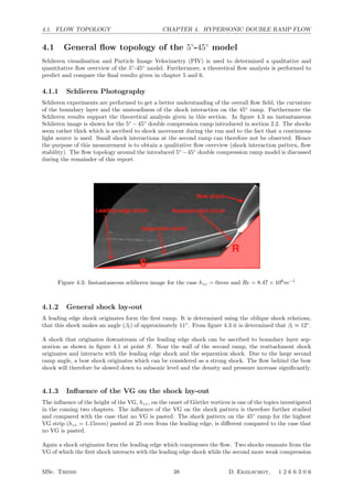
55. 4.1. FLOW TOPOLOGY CHAPTER 4. HYPERSONIC DOUBLE RAMP FLOW
Figure 4.4: Instantaneous schlieren image for the case hzz = 1.15mm and Re = 8.47 × 106
m−1
wave interacts on the merged separation and reattachment shock. This is shown in figure 4.4. The VG
creates a local stagnation point which deflects the flow upwards inducing a weak shock upfront of the
VG. In a similar fashion, a weak shock is created just downstream of the VG where the flow is deflected
downwards. The leading edge shock merges with the first VG shock and the merged shock has a shock
angle of approximately βl = 14◦
based on the Schlieren images.
Note the difference in position of the separation point S in figure 4.3 and 4.4. The separation shock
originates more downstream which indicates that the separated region is significantly smaller and more
close to the first-to-second ramp junction. This can be ascribed to the turbulent nature of the boundary
layer due to the presence of the VG. The local normal velocity gradient is higher and therefore a higher
adverse pressure gradient is needed to induce separation. Consequently, for the case of hzz = 1.15mm,
it is shown in figure 4.4 that the separation shock merges together with the reattachment shock and
interacts with the leading edge shock above the 45◦
ramp. This effect on the shock interaction above the
second ramp is noted to be the main difference between the shock patterns given in figure 4.3 and 4.4.
Similar to the case that no VG is applied, a bow shock originates above the second ramp.
4.1.4 Theoretical pressure distribution on the 5◦
− 45◦
ramp
The inviscid compressible flow domain over the 5◦
− 45◦
double compression ramp model can be theo-
retically analysed using shock polars [Delery, 1994]. The local pressure normalised by the free stream
pressure is determined. From the oblique shock relations, the Mach number, pressure, density etc. can be
obtained given the Mach number upstream of the shock and the wedge angle of the geometry. Given that
M∞ = 7.5 and the first ramp angle is 5◦
, the flow conditions downstream of the leading edge shock can
be calculated. The flow deflection induced by the separation bubble (see the blue area in figure 4.5(a))
is estimated from the Schlieren image given in figure 4.4. The separated region is modeled as an extra
ramp with θs = 12◦
based on the Schlieren image given in figure 4.4. In figure 4.5(a), the different flow
regions are indicated and three streamlines are given. The blue, green and pink streamline are used to
discuss the hodograph corresponding to the 5◦
− 45◦
model given in figure 4.5(b) and 4.5(c).
Blue stream line
The dark blue shock polar given in figure 4.5(b) corresponds to the free stream flow conditions (M0 =
M∞ = 7.5). The blue streamline passes through the leading edge shock and the pressure is increased to
(p/p0)1 = 1.35. The minor pressure rise is induced by the weak leading edge shock. Based on the oblique
shock relations, the Mach number downstream of the leading edge shock is determined to be M1 = 6.48.
The separated region is modeled as an extra ramp with θs = 12◦
based on the Schlieren image given in
figure 4.4. The pressure increases due to the weak shock originating from the separation point. Hence,
the Mach number reduces to M2 = 5.09. Further downstream, the blue streamline encounters the reat-
tachment shock which is considered to be strong due to the large deflection angle of the second ramp.
The pressure rises up to p/p0 = 120 and the total pressure reduces locally to (pt/pt,0)3 = 1.276 × 10−1
.
A local Mach number of M3 = 1.91 is calculated.
MSc. Thesis 39 D. Ekelschot, 1 2 6 6 3 0 6

56. 4.1. FLOW TOPOLOGY CHAPTER 4. HYPERSONIC DOUBLE RAMP FLOW
From figure 4.5(a) can be seen that domain 1 and 4 are connected. As a result, point 4 lies on the
intersection of the light blue shock polar (C1) and the red shock polar (C3) which indicates a small
pressure drop and thus an expansion wave (see figure 4.5(c)). The intersection lies on the strong shock
solution of the light blue shock polar. This indicates that a strong shock is present between domain 1
and 4. A similar analysis holds for the connection between domain 1 and domain (5, 6). Domain 6 is
incompatible with domain 4 and therefore there is an intermediate state present (domain 5). Point (5, 6)
is found by the intersection point of the green and dark blue shock polar shown in figure 4.5(c). For
this case the pressure drop is larger (see the green line in figure 4.5(c)) and therefore a second stronger
expansion wave originates from the shock interaction above the second ramp.
The flow passes a Prandtl-Meyer expansion going from domain 3 to domain 4. From figure 4.5(c), a change
in flow direction of 2◦
can be observed and therefore according to the Prandlt-Meyer function, M4 = 1.97.
Prandtl-Meyer expansion waves are isentropic and therefore (pt/pt,0)3 = (pt/pt,0)4,5 = (pt/pt,0)6,7,8. A
similar analogy is applied to determine the Mach number in domain 6. Based on the change in flow
direction (∆ϕ4−6 = 8◦
) which is obtained from figure 4.5(c), and the Prandlt-Meyer function the Mach
number in domain 6 is determined to be M6 = 2.19.
(a) Sketch of the 5◦ − 45◦ model with its shock pattern
−60 −40 −20 0 20 40 60 80 100
0
50
100
150
200
250
300
350
400
450
500
θ [deg]
p/p
0
4,5
6,7,8
3
21
(b) Hodograph for the 5◦ −45◦ model with a hzz = 1.15mm
at 2.5cm from the leading edge
10 20 30 40 50 60
40
60
80
100
120
140
160
180
200
220
θ [deg]
p/p
0
3
6,7,8
Expansion
wave
Expansion
wave
4,5
(c) Detail of the hodograph for the 5◦ − 45◦
Figure 4.5: Sketch of the 5◦
− 45◦
model
Table 4.1: Local Mach number for all domains
Domain 0 1 2 3 4 5 6 7 8
M 7.5 6.49 5.40 1.96 2.03 1.31 2.42 1.57 0.39
MSc. Thesis 40 D. Ekelschot, 1 2 6 6 3 0 6

57. 4.1. FLOW TOPOLOGY CHAPTER 4. HYPERSONIC DOUBLE RAMP FLOW
Green stream line
The green stream line encounters the leading edge shock. Further downstream it passes through the
combined separation/reattachment shock from domain 1 to domain 4 which is considered to be a strong
shock based on the argument given in the previous paragraphs. The pressure increases from (p/p0)1 = 10
to (p/p0)5 = 110. This is represented by the light blue shock polar connecting point 1 with point (4, 5).
A deflection angle of∆ ϕ1−5 = 40◦
is obtained. The oblique shock relations are then used to obtain
M5 = 1.2. This does not correspond with the value found in the previous paragraph forM4. The blue
stream line experienced multiple weak oblique shocks while the green stream line experienced one weak
and one very strong shock. As a result, the entropy in domain 5 differs from domain 4 causing a locally
different Mach number, velocity, temperature and density. Therefore it is expected that a slip line origi-
nates from the point where the separation and reattachment shock interact. Furthermore, the green line
passes through the expansion wave that originates from the shock interaction above the second ramp.
Due to the slip line between domain 4 and 5, a different velocity is found in domain 7 compared to domain
6.
Pink stream line
Finally, the pink stream line experiences just one strong shock. In the hodograph, this is represented by
the path at the dark blue shock polar moving from point 1 directly to point (6, 7, 8). This point lies on
the strong solution of the dark blue shock polar. The pressure increases therefore from (p/p0)0 = 1 to
(p/p0)5,6 = 65. The velocity directly behind the bow shock is expected to be lower than near the wall of
the second ramp. The flow passes through a strong (nearly normal) shock which experiences a significant
entropy drop while for the flow passing through multiple oblique shocks (see the blue and green stream
line), the entropy loss is significantly lower. Therefore the Mach number is higher near the wall (domain
6 and 7) compared to the conditions directly behind the bow shock (domain 8). As a result, another slip
line is present between domain 7 and 8. Assuming the bow shock is nearly normal, the Mach number
directly behind the bow shock is expected to be M8 = 0.39. It is therefore concluded that the flow
downstream of the bow shock is divided into three different velocity fields where the domain nearest to
the wall has the highest velocity. All local Mach numbers are also presented in table 4.1.
4.1.5 Particle Image Velocimetry (PIV) measurement campaign
Particle Image Velocimetry is used to obtain a two dimensional velocity field over the 5◦
− 45◦
ramp.
Measurements are performed for three different FOVs to increase the spatial resolution of the overall
velocity field. A sketch of the three separate FOVs is given in figure 4.6.
Figure 4.6: Overview of the domain of interest during the PIV measurement campaign
Examples of the raw and processed images for the separate FOVs are given in Appendix A. Using vector
field rotation and bilinear interpolation, the three FOVs are merged together such that an overall two
dimensional velocity field is obtained. Due to the limited time and the high work intensity of PIV in
MSc. Thesis 41 D. Ekelschot, 1 2 6 6 3 0 6

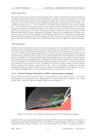
58. 4.1. FLOW TOPOLOGY CHAPTER 4. HYPERSONIC DOUBLE RAMP FLOW
the HTFD, it is chosen to determine a mean velocity field for the case that no VG is applied, at a unit
Reynolds number of 11.3 × 106
[m−1
].
Typically 30 − 40 runs are performed per FOV to obtain a converging mean of the velocity data. An
example of the converging mean for a local measurement point in the free stream in FOV 1 is given in
figure 4.7. The mean total velocity at a fixed point is plotted against the number of runs:
0 10 20 30 40
1020
1025
1030
1035
1040
1045
1050
1055
1060
# of runs [−]
V
tot,mean
[m/s]
Figure 4.7: Converging mean of Vx at a local data point in the free stream
It can be seen that the velocity converges to the free stream velocity V∞ = 1033 m/s. In figure 4.8, the
overall total velocity (Vtot) contour plot is given with the corresponding stream lines. The bow shock
is visible above the second ramp. Upstream of the bow shock, Vtot is equal to the free stream velocity
(V∞ = 1033m/s) which is also shown in more detail in figure 4.13. Furthermore, the separated flow
domain near the wall of the 5◦
is clearly visible and a clear recirculation bubble is present at the first-to-
second ramp junction. Next to that, the compression due to the reattachment shock is visualised by the
converging stream lines parallel to the second ramp.
Figure 4.8: Macroscopic flow overview by means of a contour map for Vtot. Vtot is given in m/s
Downstream of the leading edge shock, the flow travels parallel to the 5◦
ramp and a compression wave
induced by boundary layer separation deflects the flow to approximately θ = 9◦
. Hence, an increase in
Vy is expected downstream of the shock. In figure 4.9, the leading edge shock and the separation shock
are visualised by plotting a small range of Vy. From figure 4.9 can be obtained that the vertical velocity
component increases from approximately Vy,1 = 75 m/s to Vy,2 = 125 m/s.
MSc. Thesis 42 D. Ekelschot, 1 2 6 6 3 0 6

59. 4.1. FLOW TOPOLOGY CHAPTER 4. HYPERSONIC DOUBLE RAMP FLOW
Figure 4.9: Leading edge shock and separation shock indicated by the colormap of the Vy. Vy is given in
m/s
The local flow angle is calculated using Vx and Vy:
θ = arctan
Vy
Vx
(4.3)
In figure 4.10, the flow angle, downstream of the bow shock is plotted. It is shown that the flow is de-
flected parallel to the wall and thus θ ≈ 45◦
downstream of the reattachment shock where the streamlines
converge. Downstream of the bow shock, the flow is deflected slightly towards the model (θ ≈ 30◦
) which
corresponds to what is found in section 4.1.4. In the hodograph given in figure 4.5(b), it was shown
that the flow angle decreases directly behind the bow shock to ϕ6,7,8 = 39◦
. From figure 4.10 the flow
angle measured directly behind the bow shock (green domain), corresponds to ϕ6,7,8. However, more
downstream of the second ramp, the flow is deflected away from the model since θ ≈ 54◦
which differs
with what is determined in section 4.1.4. Furthermore, note that the leading edge shock and separation
shock do not interact before the bow shock. Their relative position corresponds with the Schlieren image
given in figure 4.3
Figure 4.10: Detailed colormap of the flow angle on the 45◦
ramp. Flow angle is given in degrees
MSc. Thesis 43 D. Ekelschot, 1 2 6 6 3 0 6

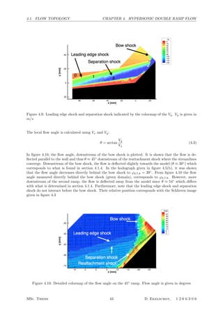
60. 4.1. FLOW TOPOLOGY CHAPTER 4. HYPERSONIC DOUBLE RAMP FLOW
In figure 4.11, a detail is given of the velocity field near the leading edge of the model. The flow domain
behind the separation shock is indicated by orange. A gradual increase of thickness is noticed of the blue
low velocity domain. Note, the typical S-shaped boundary layer velocity profile which is discussed in the
introduction of this chapter. It is therefore determined that the boundary layer is separated in figure
4.11. Hence, the upstream location where separation occurs lies outside the FOV. The length from the
start of separation with respect to the first-to-second ramp junction is estimated to be 95 mm.
Note the back flow over the complete captured length of the separated flow field at the 5◦
ramp. A
shear layer is present in the separated flow domain. Below the shear layer, a secondary boundary layer
appears and on top of the shear layer, the separated boundary layer profile is present. Again this is in
agreement with the boundary layer profile plotted in figure 4.2 and the characteristics sketched in figure
4.1.
Figure 4.11: Detail of the separation bubble upstream of the hinge line of the model. Vtot is given in m/s
In figure 4.12 a detailed, velocity field near the first-to-second ramp junction is given. The development
of a secondary boundary layer is again visible. It starts downstream on the 45◦
ramp and develops along
the geometry of the double compression ramp in positive x direction.
The white line in figure 4.12 indicates the shear layer. The radius of curvature (R = 20 mm) of is
determined based on the curvature of the shear layer as shown in figure 4.12. This number is significantly
lower than the radius of curvature found using the similar analogy as shown in [Navarro-Martinez and
Tutty, 2005]. A radius of curvature of R = 142 mm was obtained (see section 2.2). Furthermore, it
is noted that the flow is not smoothly curved over the surface, but it is slowed down abruptly by the
reattachment shock as shown by the compressed streamlines in figure 4.10.
In figure 4.13, the velocity field above the 45◦
ramp is given. For the measurement of the velocity field
above the 45◦
ramp, the x-axis of the image plane is aligned with the 45◦
ramp indicated in figure 4.6
and A.3. As a result, elongated interrogation windows are chosen in wall tangent direction so that the
spatial resolution in wall normal direction can be improved. Hence, the velocity profile behind the bow
shock and the velocity profile near the wall can be determined more accurately.
Three velocity domains are present behind the bow shock which are indicated in figure 4.13 by 1, 2,
and 3. The shock interaction results in two slip lines which divide the flow regime behind the bow shock
into three velocity regimes. This corresponds with what is determined theoretically in section 4.1.4.
Based on the velocity profile near the wall, flow expansion is measured since the flow is accelerated from
350 m/s up to 700 m/s. Directly behind the bow shock a subsonic flow domain is present where the
velocity is locally 150 − 200 m/s. The bow shock is therefore considered to be a strong shock solution
which also corresponds to the obtained solution in the hodograph given in figure 4.5(b) for the case that
hzz = 1.15 mm. Furthermore there is a low velocity domain indicated in figure 4.13 by 4. From Schlieren
visualisation and the shock polar analysis, the strong local velocity gradient is ascribed to the strong
MSc. Thesis 44 D. Ekelschot, 1 2 6 6 3 0 6

61. 4.1. FLOW TOPOLOGY CHAPTER 4. HYPERSONIC DOUBLE RAMP FLOW
Figure 4.12: Recirculation bubble near the hinge line of the model. Vtot is given in m/s
reattachment shock.
Figure 4.13: Detailed velocity field behind the bow shock on the 45◦
ramp. Vtot is given in m/s
Based on the energy equation, the local Mach number is calculated using equation 4.4:
M =
Vtot
V∞
M∞
2
+ γR
2cp
(V 2
∞ − Vtot)
(4.4)
The free stream Mach number is M = 7.5 while the Mach number behind the separation is approximately
6.0. This corresponds with what is found using the oblique shock relations (for θ1 = 5◦
, M1 = 6.48 and
θsep = 8.5◦
, M2 = 5.93). Behind the bow shock a clear subsonic domain is measured while near the wall
the Mach number again increases up to approximately M = 1.42. In table 4.2 the Mach numbers of the
four indicated domains are given:
Using shock polars, it was determined that the Mach number near the wall should be higher than the
Mach number just downstream of the bow shock. Next to that, three velocity regimes downstream of the
strong bow shock were determined in section 4.1.4. The values do not correspond which can be ascribed
to the fact that the hodograph was created for the case that Re = 14.1 × 106
[m−1
] and a VG strip of
MSc. Thesis 45 D. Ekelschot, 1 2 6 6 3 0 6

62. 4.2. RTM CHAPTER 4. HYPERSONIC DOUBLE RAMP FLOW
Table 4.2: Local Mach number for all domains
Domain 1 2 3 4
M 0.31 0.90 1.42 0.28
1.15 mm while the PIV experiments were performed for Re = 11.3 × 106
[m−1
] and no VG. The shock
interaction, as explained in section 4.1.1 is therefore slightly different.
4.2 Reference Temperature Method (RTM)
The Reference Temperature Method (RTM) can be used to determine boundary layer characteristics like
the boundary layer thickness (δ), the friction coefficient (Cf ) and the Stanton number (ch) for compress-
ible boundary layer flow using the simplified equations for incompressible boundary layers [Anderson,
2006]. A so-called reference temperature, T∗
, is determined based on the free stream Mach number and
the local temperature and used to obtain the reference flow quantities (p∗
, ρ∗
, µ∗
, etc.). From this,
the characteristic quantities can be determined by implementing the reference quantities in the known
boundary layer equations for incompressible boundary layer flow. The application of the RTM is shown
for the determination of the boundary layer thickness and the Stanton number at the 5◦
ramp of the
double compression ramp model.
As stated in section 2.2, a zig-zag Vortex Generator (VG) is used to introduce a spanwise periodic
boundary layer disturbance to induce steady longitudinal vortices. The influence of the height of the
VG on the progression of the longitudinal vortices is further investigated during this thesis project. The
boundary layer thickness is therefore determined so that the height of the VG can be scaled based on
the local boundary layer thickness. Furthermore, the Stanton number is wanted to compare a typical
measured streamwise heat flux map with the theoretically obtained streamwise heat flux map.
4.2.1 Boundary layer thickness
The boundary layer thickness is generally defined as u = 0.99ue. Examining the Blasius boundary layer
profile given in figure 4.2 more closely, it shows that at η ≈ 5 u = ue and therefore:
η = y
U
νx
= δ
Rex = 5 (4.5)
or:
δ =
5x
Rex
(4.6)
RTM relies on the available equations for incompressible flow over a flat plate. Therefore, equation 4.6
can be used to determine the boundary layer thickness for a compressible boundary layer. It is required
to determine the reference Reynolds number indicated by Re∗
x.
δ =
5x
Re∗
x
(4.7)
where:
Re∗
x =
ρ∗
Uex
µ∗
(4.8)
The flow over the first compression angle is deflected in the direction parallel to the 5◦
ramp. The free
stream Mach number is 7.5 in this example case. Using the oblique shock relations, the following flow
properties parallel at the 5◦
ramp are determined:
The reference temperature method states [Anderson, 2006]:
T∗
Tt
= 1 + 0.032M2
1 + 0.58
Tw
Te
− 1
(4.9)
MSc. Thesis 46 D. Ekelschot, 1 2 6 6 3 0 6

63. 4.2. RTM CHAPTER 4. HYPERSONIC DOUBLE RAMP FLOW
Table 4.3: Flow conditions behind the leading edge shock
M1 pt,1 [Pa] Tt,1 [K] T1 [K] p1 [Pa] ρ1 [kg/m3
]
6.48 26.3 × 105
579 61 1.02 × 103
5.81 × 10−3
The ratio between the wall temperature and the temperature at the edge of the boundary layer is
determined using the following equation:
Tw
Te
= 1 + r
γ − 1
2
M2
1 (4.10)
where r is the recovery factor and taken to be equal to r =
√
Pr =
√
0.71 = 0.83. The flow conditions at
the edge of the boundary layer are taken equal to the conditions downstream of the oblique shock. The
reference density is now determined assuming dp/dy = 0 (p∗
= p∞) and using the equation of state:
ρ∗
=
p∞
RT∗
(4.11)
where p∞ = p1. The reference viscosity coefficient, µ∗
, is calculated using Sutherlands law [Anderson,
2006]:
µ∗
µr
=
T∗
Tr
3
2
Tr + S
T∗ + S
(4.12)
In equation 4.12, µr = 1.789 × 10−5 kg
ms , Tr = 288K and S = 110. The velocity behind the shock is given
by:
Ue = M1a1 = M1
γRT1 (4.13)
At this point, the reference Reynolds number and thus the local boundary layer thickness can be evaluated
based on equation 4.8.. In this analysis, x starts from the leading edge and runs parallel with respect to
the 5◦
ramp. The VG is introduced at 25 mm from the leading edge at which the boundary thickness is
approximately 1.45 mm. The maximum VG height is hzz = 1.15 mm and therefore (hzz/δ)max = 0.92.
In figure 4.14 a detail of the boundary layer thickness is plotted against the streamwise coordinate x (blue
line). In figure 4.14, the available VG heights are indicated with different colours in the same figure. This
is done to show the size of the roughness element compared to the local boundary layer thickness.
Figure 4.14: The boundary layer thickness plotted against the streamwise coordinate s
4.2.2 Streamwise heat transfer distribution
In chapter 3 the quantity qs is introduced which represents the surface heat flux. This quantity is
numerically determined based on the measured temperature distribution as shown in section 3.2. During
the discussion of the results obtained using QIRT, typical heat transfer maps are presented. For now,
the theoretically obtained surface heat flux is compared with the measured heat flux. The heat transfer
distribution is given in figure 4.15 for the case that no VG is applied and a Reynolds number of Re =
14×106
[m−1
]. The RTM is used to evaluate the Stanton number for a laminar boundary layer. According
MSc. Thesis 47 D. Ekelschot, 1 2 6 6 3 0 6

64. 4.2. RTM CHAPTER 4. HYPERSONIC DOUBLE RAMP FLOW
to Reynolds analogy, the Stanton number is related to the friction coefficient and the Prandtl number
for a laminar incompressible boundary layer [Anderson, 2006]:
ch
Cf
=
1
2
Pr−2/3
(4.14)
The incompressible expression for cf is:
cf =
0.664
√
Rex
(4.15)
The following expression is then used to calculate c∗
h [Anderson, 2006]:
c∗
h =
0.332
Re∗
x
(Pr∗
)− 2
3 . (4.16)
where Pr∗
= µ∗
cp∗
k∗ and Re∗
x are evaluated at the reference temperature. The reference thermal conduc-
tivity is calculated using Sutherland’s law and c∗
p = 1004. In figure 4.15 the theoretically obtained ch
distribution for a 5◦
ramp angle (red line) is compared with the measured ch streamwise distribution for
a 5◦
ramp angle (blue line).
0 50 100 150
0
0.005
0.01
0.015
0.02
x [mm]
c
h
[−]
Reference Temperature Method
Measurement
Figure 4.15: Comparison between the measured ch on the 5◦
ramp and ch determined by the Reference
Temperature Method
From Reynolds analogy it is known that:
ch ∝
1
√
Res
(4.17)
where s is the streamwise coordinate from the leading edge of the model (s = 0 at x = 150, see model
coordinate system defined in section 2.2). From this point, the measured streamwise heat flux map
correspond nicely with Reynolds analogy. The boundary layer is thin at the leading edge and grows
proportionally with
√
s:
δ ∝
√
s (4.18)
The temperature gradient in normal direction becomes smaller when the boundary layer thickness in-
creases. As a result, the surface heat flux decreases with increasing boundary layer thickness and therefore,
the measured ch profile shows that it is inversely proportional to Res which corresponds to the theoreti-
cally obtained ch distribution shown in figure 4.15.
Boundary layer separation can be observed using the streamwise heat flux distribution. From figure
4.2 it is known that the du/dy decreases for a laminar boundary layer when an adverse pressure gradient
is present and the boundary layer tends to separate. The friction force decreases since:
Cf =
τw
1
2 ρu2
e
(4.19)
MSc. Thesis 48 D. Ekelschot, 1 2 6 6 3 0 6

65. 4.2. RTM CHAPTER 4. HYPERSONIC DOUBLE RAMP FLOW
where ue is the velocity at the edge of the boundary layer and τw is defined as:
τw =
µ
du
dy
w
(4.20)
At boundary layer separation, it is therefore expected to see a local decrease in Stanton number since the
ch is directly proportional to the Cf (see equation 4.14). At x = 95 mm (s = 55 mm) a local decrease
of ch is present which can be ascribed to boundary layer separation. The location of boundary layer
separation corresponds to what has been observed in the PIV images. The origin of the separation shock
was estimated to be at x = 95 mm.
To emphasise the typical local streamwise heat flux distribution, the Stanton number is multiplied by√
s such the heat flux distribution for a laminar boundary layer appears as a horizontal straight line.
Therefore ch ×
√
s is plotted against the streamwise coordinate tangent to the surface of the model in
figure 4.16 with the y-axis in log scale.
−50 0 50 100 150
10
−2
10
−1
10
0
x [mm]
c
h
[−]
Separation
Impinging shock
Reattachment
Figure 4.16: Example of a streamwise Stanton number distribution for the case of hzz = 0, Re = 14.1×106
[m−1
]
The streamwise location x = 150 mm corresponds with the leading edge while x = −80.9 mm corre-
sponds with the trailing edge of the model The decrease in ch related to boundary layer separation is
more clear in figure 4.16. The first peak near x = −24 mm is caused due to the local boundary layer
necking caused by the boundary layer reattachment. The boundary layer thickness decreases locally and
the temperature gradient in normal direction increases. The second peak in figure 4.16 near x = −45 mm
is ascribed to a shock that impinges at this location on the 45◦
ramp. The heat flux in surface normal
direction increases due to local flow compression.
From the PIV results presented in section 4.1.5, it was concluded that a secondary boundary layer
develops below the shear layer near the wall. The effect of this behaviour can be traced back in the heat
transfer map given in figure 4.16 by looking at the gradual increase in ch for 0 mm ≤ x ≤ 50 mm. In
general it can be stated that the Stanton number decreases with increasing boundary layer thickness.
However, a thin boundary layer develops just downstream of the first-to-second ramp junction. This is
seen by the locally increased ch near x = 0 mm.
In figure 4.17 the heat transfer distribution mapped on the model surface is given for the case that
no VG is applied and Re = 14.1 × 106
[m−1
].
In figure 4.17, the ln (ch) is plotted. The spanwise separation line is indicated by the dark blue line
near the leading edge figure 4.17. This line represents the same local decrease in heat transfer coefficient
shown in figure 4.16 at x ≈ 95 mm. Based on figure 4.16 and 4.17 and the undisturbed flow domain, the
boundary layer separated at x = 95 mm and reattachment takes place at x = −24 mm. Similar heat
transfer maps are presented in chapter 5.
MSc. Thesis 49 D. Ekelschot, 1 2 6 6 3 0 6

66. 4.3. VG FLOW TOPOLOGY CHAPTER 4. HYPERSONIC DOUBLE RAMP FLOW
Figure 4.17: The logarithm of the Stanton number (ch) mapped on the surface coordinate system for the
case hzz = 0mm, Re = 14.1 × 106
m−1
4.3 Flow topology around a zig-zag Vortex Generator (VG)
A zig-zag Vortex Generator (VG) strip is used to introduce a periodic spanwise boundary layer distur-
bance. The zig-zag VG is used to control the flow during the measurement since it is noticed that small
bumps on the leading edge significantly influence the stability of the flow [Schrijer, 2010a]. Hence the
zig-zag strip with λ = 6 mm is used to make sure that the longitudinal structures are steady. The flow
topology around the VG is clarified in figure 4.18.
Figure 4.18: Expected flow topology behind a zig-zag VG
The red lines indicate the streamlines over the zig-zag VG. A vortex builds up along each tooth of the
strip. The zig-zag geometry induces a spanwise velocity gradient. The flow then separates at the end of
each tooth causing a downwards velocity component which forces the flow to curl around the backwards
point zig-zig tooth. Two counter rotating vortices emanate from the backward pointing zig-zag teeth and
the velocity points away from the surface of the model indicated by the pink stream lines in figure 4.18.
The longitudinal vortices cause a movement of low momentum fluid regions away from and high mo-
mentum fluid regions towards the wall in the upwash and downwash sections respectively as shown in
figure 4.19 [Saric, 1994, Swearingen and Blackwelder, 1987]. This results in low and high speed regions
in the boundary layer in longitudinal direction which can be seen in the periodicity of the Vx velocity
component in spanwise direction. The spanwise Vx profile shows a spanwise sinusoidal behaviour.
MSc. Thesis 50 D. Ekelschot, 1 2 6 6 3 0 6

67. 4.3. VG FLOW TOPOLOGY CHAPTER 4. HYPERSONIC DOUBLE RAMP FLOW
394 SARIC
a. VortexStructure
:;:~¢::¢::::’:;::’::’-:’!i’::::::;;:’;’?:i:i:.:.:’J’:::-..-.-:’:::::::2::’:
7¢ 0 Fd2 ~ 2/r,zJX
b. NeutralPoint
C.LinearRegime
o
d. HighlyDistortedRegime
Figure 6
tortion.
Evolution of the profile dis-
velocity profile, calculated for the different streamwiselocations, and the
developmentof the highly inflectional velocity profiles that wouldgive
rise to a Rayleigh instability. The computations are for the nonlinear,
parabolized disturbance equations (Be.nmalek 1993) and should be con-
sidered as generic features that are characteristic of these distorted profiles.
Figure 9 is a comparable development of the spanwise gradients of the
velocity profiles. Theseprofiles are subject to a Kelvin-Helmholtzinsta-
bility. It is apparent that the spanwisegradients are as large as the wall-
normalgradients and that flows such as this are subject to strong secondary
instabilities.
Theother feature of this nonlinear profile distortion is saturation. At
somestreamwise location, the disturbance energy saturates as shownin
the generic Figure 10, whichshowsthe trajectories of Equation(17) for all
of the Fourier modesused in the calculation (Benmalek1993). Saturation
www.annualreviews.org/aronline
Annual Reviews
Annu.Rev.FluidMech.1994.26:379-409.Downloadedfromarjournals.annualreviews.org
byTexasAMUniversity-CollegeStationon11/30/07.Forpersonaluseonly.
(a) Orientation of the vortex motion
a. VortexStructure
:;:~¢::¢::::’:;::’::’-:’!i’::::::;;:’;’?:i:i:.:.:’J’:::-..-.-:’:::::::2::’:
7¢ 0 Fd2 ~ 2/r,zJX
b. NeutralPoint
C.LinearRegime
o
d. HighlyDistortedRegime
Figure 6
tortion.
Evolution of
velocity profile, calculated for the different streamwiseloc
developmentof the highly inflectional velocity profiles t
rise to a Rayleigh instability. The computations are for
parabolized disturbance equations (Be.nmalek 1993) and s
sidered as generic features that are characteristic of these dist
Figure 9 is a comparable development of the spanwise gra
velocity profiles. Theseprofiles are subject to a Kelvin-H
bility. It is apparent that the spanwisegradients are as larg
normalgradients and that flows such as this are subject to st
instabilities.
Theother feature of this nonlinear profile distortion is
somestreamwise location, the disturbance energy saturates
the generic Figure 10, whichshowsthe trajectories of Equati
of the Fourier modesused in the calculation (Benmalek199
Annu.Rev.FluidMech.1994.26:379-409.Downloadedfromarjournals.annualreviews.org
byTexasAMUniversity-CollegeStationon11/30/07.Forpersonaluseonly.
(b) Low momentum fluid indicated by the shaded
area and the higher momentum fluid is indicated
by the blank area
394 SARIC
a. VortexStructure
:;:~¢::¢::::’:;::’::’-:’!i’::::::;;:’;’?:i:i:.:.:’J’:::-..-.-:’:::::::2::’:
7¢ 0 Fd2 ~ 2/r,zJX
b. NeutralPoint
C.LinearRegime
o
d. HighlyDistortedRegime
Figure 6
tortion.
Evolution of the profile dis-
velocity profile, calculated for the different streamwiselocations, and the
developmentof the highly inflectional velocity profiles that wouldgive
rise to a Rayleigh instability. The computations are for the nonlinear,
parabolized disturbance equations (Be.nmalek 1993) and should be con-
sidered as generic features that are characteristic of these distorted profiles.
Figure 9 is a comparable development of the spanwise gradients of the
velocity profiles. Theseprofiles are subject to a Kelvin-Helmholtzinsta-
bility. It is apparent that the spanwisegradients are as large as the wall-
normalgradients and that flows such as this are subject to strong secondary
instabilities.
Theother feature of this nonlinear profile distortion is saturation. At
somestreamwise location, the disturbance energy saturates as shownin
the generic Figure 10, whichshowsthe trajectories of Equation(17) for all
of the Fourier modesused in the calculation (Benmalek1993). Saturation
Annu.Rev.FluidMech.1994.26:379-409.Downloadedfromarjournals.annualreviews.org
byTexasAMUniversity-CollegeStationon11/30/07.Forpersonaluseonly.
(c) The VG/initial disturbance causes fluctuations
in the momentum distribution
a. VortexStructure
:;:~¢::¢::::’:;::’::’-:’!i’::::::;;:’;’?:i:i:.:.:’J’:::-..-.-:’:::::::2::’:
7¢ 0 Fd2 ~ 2/r,zJX
b. NeutralPoint
C.LinearRegime
o
d. HighlyDistortedRegime
Figure 6
tortion.
Evolution o
velocity profile, calculated for the different streamwiselo
developmentof the highly inflectional velocity profiles
rise to a Rayleigh instability. The computations are for
parabolized disturbance equations (Be.nmalek 1993) and
sidered as generic features that are characteristic of these dis
Figure 9 is a comparable development of the spanwise gr
velocity profiles. Theseprofiles are subject to a Kelvin-H
bility. It is apparent that the spanwisegradients are as lar
normalgradients and that flows such as this are subject to s
instabilities.
Theother feature of this nonlinear profile distortion is
somestreamwise location, the disturbance energy saturate
the generic Figure 10, whichshowsthe trajectories of Equat
of the Fourier modesused in the calculation (Benmalek19
Annu.Rev.FluidMech.1994.26:379-409.Downloadedfromarjournals.annualreviews.org
byTexasAMUniversity-CollegeStationon11/30/07.Forpersonaluseonly.
(d) Mushroom shaped distribution is formed
Figure 4.19: Evolution of the secondary instability [Saric, 1994]
A typical spanwise velocity profile is given in figure 4.20 where Vy represents the spanwise velocity
component and Vz the wall normal velocity component. As a result, a high velocity regime is present
where the velocity vector points towards the surface of the model. This results in longitudinal streaks
of locally low and high momentum regimes. Local heat loss occurs when the kinetic energy increases
based on the conservation of energy. The heat transfer coefficient and thus the Stanton number increases
locally. Hence near wall high kinetic longitudinal streaks induce higher heat flux levels. The longitudinal
high velocity domain can therefore be identified using QIRT. Based on figure 4.18, a periodic spanwise
heat transfer distribution is expected as shown by a sketch of the spanwise q distribution in figure 4.20.
Not much is known about the persistence of the introduced disturbances and what kind of flow structures
are present behind this particular VG. Therefore Elsinga and Westerweel [2012] performed research on
the flow around a similar zig-zag strip by means of Tomographic Particle Image Velocimetry (Tomo-PIV)
in subsonic flow (V = 0.21 m/s). Streak-like structures are obtained directly behind the strip. Further-
more, back flow is noticed in the near-wall part of the boundary layer directly behind the strip. This is
shown in figure 4.21(a). In figure 4.21(b) the velocity field is plotted in the (y, z) plane at x = x
δ0
where
δ0 is the undisturbed boundary layer thickness. Note the cross flow which is caused due to the yaw angle
of approximately 5◦
that the VG makes with respect to the oncoming flow.
Elsinga and Westerweel [2012] concluded that behind each downstream pointing tip a low velocity domain
and behind each upstream pointing tip of the VG a high velocity domain is present. This corresponds
with the sketch given in figure 4.18 and the results found by Sch¨ulein and Trofimov [2011].
Near the point of average reattachment, the spanwise vortices break up into arches and subsequently
form hairpin-like structures. Furthermore it was noted that the average velocity field differs significantly
from the instantaneous snap shots. Instead of spanwise vortices, the meain co-rotating streamwise vortices
were measured directly behind the VG. The lack of symmetry is explained by the previously discussed
yaw-angle of the trip strip.
Sch¨ulein and Trofimov [2011] performed research regarding hypersonic flow over a flat plate with down-
stream, a ramp with varying wedge angles (20◦
, 25◦
or 30◦
). The length of the flat plate is 500 mm.
The distance between the ramp and the leading edge of the flat plate is indicated by xs. The distance
xs could be varied between 225 mm and 475 mm. The second compression ramp has a length of 300
mm and the complete model has a width of 400 mm. Experiments were performed at two free stream
MSc. Thesis 51 D. Ekelschot, 1 2 6 6 3 0 6

68. 4.3. VG FLOW TOPOLOGY CHAPTER 4. HYPERSONIC DOUBLE RAMP FLOW
Figure 4.20: The expected Vy and Vz distribution together with the expected surface heat flux
(a) Three-dimentional rendering of the mean velocity field
showing back flow (blue) and vortical motion.
(b) Velocity vectors in the cross plane x
δ0
= 3.05.
Figure 4.21: Results regarding the flow topology around zig-zag in subsonic flow by Elsinga and Wester-
weel [2012]
MSc. Thesis 52 D. Ekelschot, 1 2 6 6 3 0 6

69. 4.3. VG FLOW TOPOLOGY CHAPTER 4. HYPERSONIC DOUBLE RAMP FLOW
Mach numbers namely at M∞ = 3 with T0 = 260K, P0 = 0.32 MPa and a unit Reynolds number of
Re = 30 × 106
m−1
and at M∞ = 5, T0 = 400K, P0 = 2.55 MPa and Re = 45 × 106
m−1
.
The difference between two different VGs, a zigzag strip and a single triangular prism, were investi-
gated. The height and the wavelength of the VG were varied in combination with the position of the VG
with respect to the leading edge. Sch¨ulein and Trofimov [2011] applied a mineral oil with TiO2 pigment
powder on the surface to visualize the streamlines near the wall.
Oil flow visualisation relies on the no-slip condition at the wall, the velocity and shear stress at air-
oil interface are continuous and a balance is present between the viscous forces and the pressure gradient.
Hence, the flow direction in oil depends on the wall shear stress and the pressure gradient [Scarano, 2007].
In figure 4.22 a typical skin friction pattern is given for the separated flow domain.
14 E. Sch¨ulein and V. M. Trofimov
Triangular prism
Wake vortex pair
Low-velocity streak
High-velocity streak
Turbulent wedges
Longitudinal vortices
Low-velocity streak
High-velocity streak Ramp leading edge
B
A
B
Separation line Reattachment line
Horseshoe vortex pair(a)
(b)
Figure 9. Proposed effect of single prism-type vortex generator. (a) Estimated effect of
longitudinal disturbances, generated by the triangular prism, on the laminar–turbulent
transition. (b) Further development of the vortical disturbances, leading to the formation
of longitudinal vortices near the separation region.
3.3. Influence of the relative size of a single LPVG on the downstream flow topology
The vortical structure in the presence of a triangular-prism VG and its assumed effect
on the flow topology generated far downstream near the ramp are sketched in figure 9.
Figure 9(a) demonstrates the estimated effect of longitudinal disturbances, generated
by the triangular prism, on the laminar–turbulent transition process via generation,
growth and breakdown of steady streamwise streaks in the laminar boundary layer
with formation of turbulent wedges.
In the next stage of the flow development (figure 9b), the existing vortical
disturbances start a new self-sustaining process in the turbulent boundary layer, which
is accompanied by formation and amplification of steady streaky superstructures,
leading finally to the reappearance of longitudinal vortices in the ramp flow. In some
sense, each vortex pair induced near the reattachment region on the ramp is a child of
a vortex pair, which was generated originally by the VG or by the roughness element
near the leading edge.
(a) 3D overview of separation and reattachment found by
Sch¨ulein and Trofimov [2011]
16 E. Sch¨ulein and V. M. Trofimov
S3
N1 N2
S2
S4
S1
Separation line Reattachment line
S3
N4
N3
N1
S5
N2
S6
S2
S4
S1
Separation line Reattachment line
S5
N2
N1
S1
N3
S2
S4
S3
Reattachment lineSeparation line
λ
λ
λ
Figure 10. Interpretation of the skin-friction pattern in the separation region of the ramp flow
obtained experimentally. The sketches presented correspond to, from top to bottom, streaky
disturbances of increasing amplitude in the upstream boundary layer. This effect was achieved
in the experiments by variation of the parameters hg and xs: higher hg and shorter xs cause
more intense disturbances.
(b) Oil visualization indicating the skin friction pattern be-
tween the separation and reattachment line. The above im-
pression is for the case of small λ
δ
and a long 5◦ ramp found
by Sch¨ulein and Trofimov [2011]
Figure 4.22: Results regarding the flow topology around zig-zag in subsonic flow by Sch¨ulein and Trofimov
[2011]
The horizontal lines connecting S2 with S4 and S1 with S3 represent local reattachment lines. The sep-
aration line and reattachment lines are indicated in the figure. In between those lines, the separated
flow domain is shown where overall back flow is present. The shape of the separation line is influenced
by the upstream VG indicated by the wavy spanwise separation line. Furthermore, downstream of the
reattachment line, a diverging streamline pattern is noticed.
It is found that the dimensions of the VG have an influence on the intensity of separation. Sch¨ulein
and Trofimov [2011] show that for large h
δ , where δ is the boundary layer thickness and h the height of
the VG, and a short xs, the intensity of the vortical disturbance is high. The flow is then characterised by
the formation of a secondary separation bubble with a pair of focus points inside the separation bubble
indicated in figure 4.22(a).
Sch¨ulein and Trofimov [2011] measured coherent longitudinal so-called superstructures in undisturbed
turbulent boundary layers as unsteady longitudinal clusters. However, when the boundary layer is tripped
by a VG, these superstructures become steady. It is stated that downstream of the VG, a vortical distur-
bance is present after which a transition takes place into self-sustained superstructures. These longitudinal
superstructures are amplified and the formation and reappearance of longitudinal vortices occurs on the
45◦
ramp.
Sch¨ulein and Trofimov [2011] also investigated the influence of the angle of the compression ramp on
the wavelength of the longitudinal vortices in combination with the boundary layer thickness. It is
found that the vortex wavelength increases when the second ramp angle is increased from θ2 = 20◦
to
θ2 = 25◦
. The superstructures are amplified at reattachment and due to the increase of compression
angle, the size of the separation bubble increases together with the streamwise pressure gradient and
pressure jump. These parameters amplify the induced disturbance, hence, an increase of vortex intensity
in the streamwise scale of the structure is measured.
MSc. Thesis 53 D. Ekelschot, 1 2 6 6 3 0 6

70. 4.4. G ¨ORTLER INSTABILITY CHAPTER 4. HYPERSONIC DOUBLE RAMP FLOW
4.4 G¨ortler instability
G¨ortler vortices are induced by the centrifugal forces associated with the change in direction of motion
forced on the fluid by the geometry of the surface. The viscous boundary layer flow fulfills the no-slip
condition when a flow propagates over a wall. The curvature of the wall leads to an unstable situation
depending on the local velocity profile and the local radius of curvature. Figure 4.23 presents an example
of the contradictory flow situation which induces the G¨ortler instability:
Annu.Rev.FluidMech.1994.26:379-409.Downloadedfromww
byTechnischeUniversiteitDelfton06/13/12.Forperson
Figure 4.23: Instable flow situation causing the G¨ortler instability. Figure taken from Saric [1994]
From mechanics it is known that the angular velocity increases with increasing radius of curvature which
is in conflict with the no-slip condition at the wall. This instability causes a longitudinal vortex structure
in the boundary layer which is often referred to as G¨ortler vortices. Mathematically, this instability is
prescribed by the Rayleigh criterion which is defined in equation 4.21 [Saric, 1994]. IfΓ( r) = rV (r):
dΓ2
dr
0 (4.21)
The influence of the wall radius of curvature on the behaviour of the boundary layer flow is discussed.
The general assumptions that are taken into account in this section are:
• The boundary layer thickness is much smaller than the radius of curvature (δ/R 1)
• The basic flow is nearly parallel to the wall which means that centrifugal effects are
neglected in the description of the basic flow, although, they are partially retained in
the disturbance equations.
• A local stability analysis is considered for which the basic flow is assumed to be inde-
pendent of the streamwise and wall normal coordinate
Consider the double compression ramp model as an obstacle which forces the flow to curve. Yet, the no-
slip condition holds at the surface of the model. Therefore, a similar instability as in figure 4.23 occurs
in double compression ramp flow. The curvature of the flow is therefore simplified by taking the red
curved plane as shown in figure 4.24(b). The red curved plane indicates the space where the boundary
layer is separated. Point S indicates the separation line and A the reattachment line. R indicates the
radius of curvature over which the flow is turned. The coordinate system shown in figure 4.24(b) is used
to investigate the characteristic flow properties for G¨ortler instabilities. For now the radius of curvature
is taken to be constant but for a double compression ramp this will not be the case [Navarro-Martinez
and Tutty, 2005].
In figure 4.24(b), x = Rθ, y = R−r and z is the spanwise coordinate. Using the following non-dimensional
coordinates:
¯x = x
L , ¯y = y
δ , ¯z = z
δ
MSc. Thesis 54 D. Ekelschot, 1 2 6 6 3 0 6

71. 4.4. G ¨ORTLER INSTABILITY CHAPTER 4. HYPERSONIC DOUBLE RAMP FLOW
d thermography [9]. It was found that the interaction was transitional (laminar at
ent) and inside the separated region the flow was highly three dimensional [8].
ements by means of stereo-PIV and infrared thermography showed the presence of
ear layer indicating the presence of Görtler vortices which increases the surface heat
per the effect of the Reynolds number and second ramp angle on the occurrence of
experiments initial disturbances are generated which are in turn amplified by the
reated with different spatial wavelengths (in span-wise direction) to investigate the
er a double compression
5
Fig. 2. Schematic of Görtler vortices in a
boundary layer over a concave wall [saric]
(a) Sketch of G¨ortler vortices together with a typical
boundary layer profile and a curved geometry Saric
[1994]
(b) The defined coordinate system that is used during
the local linear stability analysis
Figure 4.24: Sketch of G¨ortler vortices in a boundary layer and a sketch of the model with cylindrical
coordinate system
and assuming that L δ, the Navier Stokes equations are given in cylindrical coordinates. The cylindrical
N-S equations are linearised in the following way and as a result, the following equations are obtained:
u
u∞
= u(¯x, ¯y) + ξu(¯x, ¯y, z) + O(ξ2
)
v
Re
u∞
= v(¯x, ¯y) + ξv(¯x, ¯y, z) + O(ξ2
)
w
Re
u∞
= ξw(¯x, ¯y) + O(ξ2
)
p
ρu2
∞
Re2
= p(¯x)Re2
+ p0(¯x, ¯y) + ξp
(¯x, ¯y, ¯z) + O(ξ2
)
and applying an order estimation, the following is obtained for the free stream: [Goulpie et al., 1996,
Batchelor and Miles, 1981]:
O(1):
∂u
∂¯x
+
∂v
∂¯y
= 0 (4.22)
u
∂u
∂¯x
+ v
∂u
∂¯y
= −
∂p
∂¯x
+
∂2
u
∂¯y2
(4.23)
u
∂v
∂¯x
+ v
∂v
∂¯y
= −
∂p0
∂¯y
+
∂2
v
∂¯y2
− (Gu)
2
(4.24)
For the perturbation terms of order O(ξ) where O(ξ) O(1) holds:
O(ξ):
∂u
∂¯x
+
∂v
∂¯y
+
∂w
∂¯z
= 0 (4.25)
u
∂u
∂¯x
+ u ∂u
∂¯x
+ v
∂u
∂¯y
+ v ∂u
∂¯y
=
∂2
u
∂¯y2
+
∂2
u
∂¯z2
(4.26)
MSc. Thesis 55 D. Ekelschot, 1 2 6 6 3 0 6

72. 4.4. G ¨ORTLER INSTABILITY CHAPTER 4. HYPERSONIC DOUBLE RAMP FLOW
u
∂v
∂¯x
+ u ∂v
∂¯x
+ v
∂v
∂¯y
+ v ∂v
∂¯y
= −
∂p
∂¯y
+
∂2
v
∂¯y2
+
∂2
v
∂¯z2
− 2G2
uu
(4.27)
u
∂w
∂¯x
+ v
∂w
∂¯y
= −
∂p
∂¯z
+
∂2
w
∂¯y2
+
∂2
w
∂¯z2
(4.28)
Equation 4.24 shows that a pressure gradient in normal direction balances the centrifugal term (Gu)2
.
The influence of the local radius of curvature is incorporated in the G¨ortler number which is defined as:
G = Re
R
L
(4.29)
Saric [1994], Goulpie et al. [1996], Bottaro and Luchini [1999] performed a linear stability analysis in
which the perturbation quantities are given by (¯u, ¯v, ¯w, ¯p) = (ˆu(y), ˆv(y), ˆw(y), ˆp(y))eσx+iβz
where σ is the
growth rate of the vortices and β is the spanwise wavenumber . Equations 4.25-4.28 are rewritten such
that:
L(σ, G,β ) ˆf = λ ˆf = 0 (4.30)
where ˆf = (ˆv(y), ˆu(y)) is the eigenvector and L is a linear operator which depends on (U, V, P, β,σ ).
(U, V, P) are determined by using the Falkner-Skan equation which is solved numerically using the Euler
shooting method. The derivation of the entries of the linear operator L are given in Appendix B
−0.4 −0.2 0 0.2 0.4 0.6 0.8 1
0
1
2
3
4
5
6
7
8
u/U
η=y(U/(νx))1/2
(a) Solution to the Falkner-Skan equation from which U, Uy
and Uyy are locally determined
10
0
10
1
10
2
β [−]
G[−]
(b) Stability plot in the β − G plane for the case of γ = 0
and η = 1
Figure 4.25: Stability plot [Ekelschot, 2012]
Assuming that the G¨ortler vortices propagate in the top part of the boundary layer, the stability plot is
shown for a typical boundary layer profile at separation given in figure 4.25(a) at η = 1. The wavelength
of the VG is fixed since λzz = 6 mm. Assuming a G¨ortler number of 100 and β is given in equation 4.31:
β =
2πξL
λ
=
2π 1
100 115
6
= 1.20 (4.31)
where ξ ≈ 1
R , L is a reference length which in this case is equal to the width of the model. In figure
4.25(b), the stability plot is given in the (β, G) plane. The red lines represent positive growth rates.
The most positive red line represents the highest σ and the black line represents σ = 0 (neutral curve).
Hence the absolute value of the growth rate approaches zero for the red or blue lines that are closer to
the neutral curve. The blue lines represent the negative growth rates. From figure 4.25(b) it can be seen
that the point (1.20, 100) in the (β, G) plane, lies above the neutral curve, hence, a positive growth rate
is expected based on the linear stability analysis. The reproduction of the local linear stability analysis is
performed as an exercise during the literature study phase of this thesis project. A comparison is made
between a Blasius boundary layer profile and a typical boundary layer profile at separation for different
η. The results are presented in Ekelschot [2012].
MSc. Thesis 56 D. Ekelschot, 1 2 6 6 3 0 6

73. 4.5. G ¨ORTLER VORTICES CHAPTER 4. HYPERSONIC DOUBLE RAMP FLOW
4.5 G¨ortler vortices
In this section the previously performed research is discussed. The valuable characteristic numbers are
presented which are used to compare experimental and computational results. As a result, this section
emphasises the contribution of this thesis to field of G¨ortler instabilities in hypersonic flow.
Schrijer [2010a] performed Quantitative Infrared Thermography (QIRT), Schlieren photography, and Par-
ticle Image Velocimetry (PIV) experiments on double compression ramp flow in the HTFD at M = 7.5.
The free stream flow conditions are therefore similar to the conditions present during the measurement
described in this thesis. Two double compression ramp configurations are compared. The two configura-
tions are given in the test matrix given below:
Table 4.4: Dimensions of the two tested configurations test by Schrijer [2010b,a]
L1 [mm] ˆθ1 [◦
] L2 [mm] ˆθ2 [◦
]
Configuration 1 96 15 66 30
Configuration 2 96 15 81 45
The model has a width of 115 mm. The unit Reynolds number is changed from 5 × 106
[m−1
] to 11 × 106
[m−1
] . The total temperature is constant and equal to Tt = 579K similar to the cases that are presented
during this thesis.
With Schlieren photography and PIV, the flow topology is determined. It is found that for the first
configuration, an Edny type VI interaction is present while for the second configuration a Edney type V
interaction as shown in figure 4.26(a) and 4.26(b), respectively.
X [mm]
Y[mm]
-100 -50 0 50
0
20
40
60
80
750 795 840 885 930 975 1020
|V| [m/s]
slip line
separation shock
reattachment shock
combined shock
leading edge shock
expansion wave
X [mm]
Q[kW/m
2
]
-100 -50 0 50
0
25
50
75
100
Figure 5.7: Average PIV (a), schlieren (b) and QIRT (c) results for the 15-30 wedge
model
measurements. The same situation applies for the 15◦
-45◦
configuration discussed in
the next section.
From the local value of the velocity, the Mach number can be computed under the
assumption of adiabatic flow (constant total temperature), which is a justified ap-
proach for the present flow field if the boundary layer is excluded. The expression for
the Mach number can be derived combining the definition for the Mach number M
and the energy conservation equation resulting in:
72
(a) Schlieren and PIV results for the second config-
uration ˆθ1 = 15◦ ˆθ2 = 30◦
X [mm]
Q[kW/m
2
]
-100 -50 0 50
0
50
100
150
X [mm]
Y[mm]
-100 -50 0 50
0
20
40
60
80
100 250 400 550 700 850 1000
|V| [m/s]
leading edge shock
separation shock
curved shock
reattachment shock
Figure 5.13: Average PIV (a), schlieren (b) and QIRT (c) results for the 15-45 wedge
model
at the intersection of the leading edge shock and curved shock, which is connected
to the oblique reattachment shock by a Mach stem (strong shock solution). The
theoretical (inviscid) pattern agrees with the experimental visualisation, albeit that
the Mach stem is not very evident in the schlieren image. As a result of the complex
interaction, at least two distinct regions are formed in the flow downstream: a region
close to the wall where the flow has passed multiple oblique shocks (lower entropy
loss), and a second region behind the curved shock. After subsequent expansion, the
flow in the former region (region 4) develops into a wall-jet, with significantly higher
momentum than the flow further away from the wall. This flow topology is found to
be in agreement with Olejniczak et al. [61].
76
(b) Schlieren and PIV results for the second con-
figuration ˆθ1 = 15◦ ˆθ2 = 45◦
Figure 4.26: PIV results obtained by Schrijer [2010a]
PIV measurements are performed to obtain a general flow description for the 15◦
− 30◦
and a 15◦
− 45◦
model given in table 4.4. Leading edge irregularities caused an irregular spanwise boundary layer sepa-
ration which caused an inaccurate measurement of the separation bubble.
The heat flux distribution over the surface is determined by means of QIRT. As a result it is found
that the maximum heat flux at reattachment is comparable with the result found by Navarro-Martinez
and Tutty [2005] namely∆ qmax = 18.73%. A slightly adjusted definition of the growth rate is determined
where not the maximum but the mean amplitude is taken at separation and at reattachment. The ratio
of the spanwise heat transfer fluctuations at reattachment and at separation is defined as the growth rate.
MSc. Thesis 57 D. Ekelschot, 1 2 6 6 3 0 6

74. 4.5. G ¨ORTLER VORTICES CHAPTER 4. HYPERSONIC DOUBLE RAMP FLOW
σ =
∆qr
∆qs
(4.32)
where∆ qs,max represents the spanwise heat transfer fluctuations at separation and∆ qr,max the spanwise
heat transfer fluctuations at reattachment. The G¨ortler number is defined based on the boundary layer
thickness δ defined in equation 4.33:
Gδ = Reδ
δ
R
(4.33)
The spanwise wavelength of the VG is varied and the influence on the growth rate and G¨ortler number
are discussed. Therefore the non dimensional wavelength parameter is defined in equation 4.34 [Schrijer,
2010b]:
Λ = Reλ
λ
R
(4.34)
The wavelength of the VG is varied and the growth rate, σ is plotted against Gδ for both configurations
in figure 4.27. It is found that the growth rate decreases with increasing G¨ortler number. This can be
explained by the fact that an increase in G¨ortler number means also an increase in Reynolds number
which means that the longitudinal vortices break up more easily leading to lower measured fluctuations.
Schrijer [2010b] related the non dimensional wavenumber, the growth rate and the G¨ortler number and
Fig. 7. Typical heat flux map for 15
o
-45
o
model including
= 2 mm element
Fig. 8. Schlieren image of the flow over the 15
o
-45
o
model
including the = 2 mm element
In Figure 7 a typical heat flux map is shown for the 15
o
-45o
model with the 2 mm wavelength elements. Comparing
this map to the heat flux profile for the clean model, it can be seen that the overall flow features such as the double peak at
reattachment are unaltered. However the effect of the comb-shaped element on the flow field is clearly visible in the form of
span-wise oscillations in the heat flux. Directly downstream of the element (y 50 mm in Figure 7) the oscillations are clearly
visible however further downstream the effect decreases. This is due to the increase in boundary layer thickness when
moving downstream and the fact that the fact that the vortices are mainly located in the upper part of the boundary layer. The
effect of the element can also be observed from the schlieren image, see Figure 8. From the visualization it can be seen that
the element only has a limited effect on the flow field (only weak waves are generated by the element) and the overall
features are similar to those observed for the clean model.
Fig. 9. Görtler number versus growth rate for the
15o
-30
o
Fig. 10. Görtler number versus growth rate for the
15configuration o
-45
o
In Figure 9, the results are presented in a Görtler number versus wavelength diagram for the 15
o
-30
o
model and
Figure 10 shows the diagram for the 15
o
-45
o
model. It can be seen that the amplification rates decrease with increasing
Görtler number. And for sufficiently high Görtler numbers even a plateau is reached. This is opposite to the trend found in [5]
and [6], although those experiments reported considerably lower Görtler numbers. A possible explanation for the decrease in
the growth rate can be found in the fact that an increase in Görtler number also means an increase in Reynolds number. For
the higher Reynolds numbers the vortices are broken-up more easily and therefore lower fluctuations are measured.
Furthermore it can be seen that the growth rates measured for the 15
o
-45o
model are considerably larger than for the 15o
-30o
configuration(a) Growth rate plotted against the G¨ortler number
for three different wavelengths for the 15◦ − 30◦ con-
figuration
Fig. 7. Typical heat flux map for 15
o
-45
o
model including
= 2 mm element
Fig. 8. Schlieren image of the flow over the 15
o
-45
o
model
including the = 2 mm element
In Figure 7 a typical heat flux map is shown for the 15
o
-45o
model with the 2 mm wavelength elements. Comparing
this map to the heat flux profile for the clean model, it can be seen that the overall flow features such as the double peak at
reattachment are unaltered. However the effect of the comb-shaped element on the flow field is clearly visible in the form of
span-wise oscillations in the heat flux. Directly downstream of the element (y 50 mm in Figure 7) the oscillations are clearly
visible however further downstream the effect decreases. This is due to the increase in boundary layer thickness when
moving downstream and the fact that the fact that the vortices are mainly located in the upper part of the boundary layer. The
effect of the element can also be observed from the schlieren image, see Figure 8. From the visualization it can be seen that
the element only has a limited effect on the flow field (only weak waves are generated by the element) and the overall
features are similar to those observed for the clean model.
Fig. 9. Görtler number versus growth rate for the
15o
-30
o
Fig. 10. Görtler number versus growth rate for the
15configuration o
-45
o
In Figure 9, the results are presented in a Görtler number versus wavelength diagram for the 15
o
-30
o
model and
Figure 10 shows the diagram for the 15
o
-45
o
model. It can be seen that the amplification rates decrease with increasing
Görtler number. And for sufficiently high Görtler numbers even a plateau is reached. This is opposite to the trend found in [5]
and [6], although those experiments reported considerably lower Görtler numbers. A possible explanation for the decrease in
the growth rate can be found in the fact that an increase in Görtler number also means an increase in Reynolds number. For
the higher Reynolds numbers the vortices are broken-up more easily and therefore lower fluctuations are measured.
Furthermore it can be seen that the growth rates measured for the 15
o
-45o
model are considerably larger than for the 15o
-30o
configuration(b) Growth rate plotted against the G¨ortler number
for three different wavelengths for the 15◦ − 45◦ con-
figuration
Figure 4.27: Growth rate plotted against the G¨ortler number for three different wavelengths for the two
configurations presently discussed [Schrijer, 2010b]
plotted them for both configurations. These plots are shown in figure 4.28. It is found that the lines for
constant spanwise wavelength, λ, in the Gδ − Λ plane are straight with a slope of 3/2. A subtle trend is
seen of an increase in growth rate with the wavelength parameter.
Luca de et al. [1993] investigated G¨ortler instabilities in a hypersonic boundary layer (M=7) by means
of QIRT experiments. This is done by looking at a flat plate at zero angle of attack which is followed by
a concave wall with a constant radius of curvature (see figure 4.29(a)). Three different cases are tested:
Table 4.5: Dimensions of the two tested configurations test by Luca de et al. [1993]
L1 [mm] L2 [mm] R [mm]
Model A 50 150 2000
Model B 50 120 1000
Model C 100 100 1000
MSc. Thesis 58 D. Ekelschot, 1 2 6 6 3 0 6

75. 4.5. G ¨ORTLER VORTICES CHAPTER 4. HYPERSONIC DOUBLE RAMP FLOW
model. For example at G
o
-30
o
model and around 3 to 4 for the 15
o
-45
o
model.
Fig. 11. Görtler number versus wavelength
parameter for the 15o
-30o
Fig. 12. Görtler number versus wavelength
parameter for the 15configuration, the labels indicate
the growth rate
o
-45o
configuration, the labels indicate
the growth rate
Finally in Figures 11 and 12, the diagrams for the Görtler number versus wavelength parameter are given for both models.
The labels in the diagram indicate the growth rate. Lines for constant are straight with a slope of 3/2. Opposite to the trend
observed for the Görtler number, the growth ratio seems increase with the wavelength parameter, although the trend is not
so clear. Furthermore it can be clearly observed that the current measurements are performed for relatively high wavelength
parameters and that, in order to find the maximum amplification wavelength, should be decreased further.
5. Conclusions
The occurrence of Görtler vortices on a double compression ramp in a Mach 7.5 hypersonic flow is investigated by
means of infrared thermography. The results are presented in the form of scaling parameters that are obtained from normal
mode analysis. In the experiments comb-shaped elements are used to generate vortices near the leading edge of the model
that are either amplified or damped by the instability mechanism responsible for the generation of Görtler vortices. The span-
wise wavelength of the vortices is varied by using different elements. The growth rate of the vortices is inferred from the heat
transfer measurements. From the experiments it can be shown using schlieren visualization and IR thermography that the
comb-shaped element, apart from generating the vortices, only has a local influence on the flow field and that the overall flow
features are not affected.
Comparing the results for the 15o
-30
o
model to the 15
o
-45
o
model it is found that the growth rate is larger for the
latter. Furthermore for both models the growth rate of the vortices decreases with the Görtler number and increases with the
wavelength pattern. However in the latter case the trends is less obvious. The current results show the opposite trend to that
observed in literature. An explanation for this can found in the fact that the Görtler numbers in the current experiments were
considerably larger than those in literature. An increase in Görtler number also means an increase in Reynolds number and
apparently the Reynolds number becomes so high that the vortices diffuse hence decreasing the growth rate.
(a) G¨ortler number plotted against the wavelength
parameter for the 15◦ − 30◦ configuration where the
labels indicate the growth rate
model. For example at G o
-30o
model and around 3 to 4 for the 15o
-45o
model.
Fig. 11. Görtler number versus wavelength
parameter for the 15
o
-30
o
Fig. 12. Görtler number versus wavelength
parameter for the 15configuration, the labels indicate
the growth rate
o
-45
o
configuration, the labels indicate
the growth rate
Finally in Figures 11 and 12, the diagrams for the Görtler number versus wavelength parameter are given for both models.
The labels in the diagram indicate the growth rate. Lines for constant are straight with a slope of 3/2. Opposite to the trend
observed for the Görtler number, the growth ratio seems increase with the wavelength parameter, although the trend is not
so clear. Furthermore it can be clearly observed that the current measurements are performed for relatively high wavelength
parameters and that, in order to find the maximum amplification wavelength, should be decreased further.
5. Conclusions
The occurrence of Görtler vortices on a double compression ramp in a Mach 7.5 hypersonic flow is investigated by
means of infrared thermography. The results are presented in the form of scaling parameters that are obtained from normal
mode analysis. In the experiments comb-shaped elements are used to generate vortices near the leading edge of the model
that are either amplified or damped by the instability mechanism responsible for the generation of Görtler vortices. The span-
wise wavelength of the vortices is varied by using different elements. The growth rate of the vortices is inferred from the heat
transfer measurements. From the experiments it can be shown using schlieren visualization and IR thermography that the
comb-shaped element, apart from generating the vortices, only has a local influence on the flow field and that the overall flow
features are not affected.
Comparing the results for the 15o
-30o
model to the 15o
-45o
model it is found that the growth rate is larger for the
latter. Furthermore for both models the growth rate of the vortices decreases with the Görtler number and increases with the
wavelength pattern. However in the latter case the trends is less obvious. The current results show the opposite trend to that
observed in literature. An explanation for this can found in the fact that the Görtler numbers in the current experiments were
considerably larger than those in literature. An increase in Görtler number also means an increase in Reynolds number and
apparently the Reynolds number becomes so high that the vortices diffuse hence decreasing the growth rate.
(b) G¨ortler number plotted against the wavelength
parameter for the 15◦ − 45◦ configuration where the
labels indicate the growth rate
Figure 4.28: G¨ortler number plotted against the wavelength parameter for the two configurations
presently discused [Schrijer, 2010b]
The unit Reynolds numbers ranges from 0.89×107
m−1
to 1.91×107
m−1
and the Tt = 800K. The ampli-
tude in heat flux with respect to the spanwise mean distribution increased in downstream direction. No
initial disturbance is introduced and the heat flux distribution on the surface of the model is determined.
Sinusoidal fluctuations are obtained in spanwise direction which is an indication for the longitudinal vor-
tex structures. The spanwise fluctuations have an average wavelength of 8 mm. In the stability plot,
given in figure 4.29(b), the models are plotted and it can be seen that they are not located on the side
where all the vortices will be amplified. The spanwise wavenumber β = 2πλ
δ where δ is boundary layer
(a) The model with characteristic dimensions used by
Luca de et al. [1993]
9 /k Model a ~ / .
~.Model b~ .,,, ./, //'
30 [] Modelc ..~ ..
5 ^/ //
3
Fig. 5. Correlation ofpresent experimental data as compared to the
stability diagram of Aymer et al. (1991)for M = 7 and Tw/Taw=0.5
As is evident, all the experimental points are located in
the region where the disturbances have to be amplified
according to the linear theory (note that a stable flow is
predicted for Goertler numbers less than 1.6). The straight
line for A = 1800 (dotted line) is also reported in Fig. 5. As
predicted by Aymer et al. (1991), this value corresponds to
the wavelength that maximizes the total amplification
and is practically independent of the final Goertler
number Go (i.e., of the streamwise location x). Such a par-
ticular wavelength should be correlated to the one actual-
ly observed in the experiments. However, as already dis-
cussed in the introduction, any external factor imposed on
the flow may affect the activation of the instability mech-
anism. Hence, depending on the particular experimental
apparatus (e~g. nozzle, wind tunnel screens, model), only
the disturbances characterized by a certain wavelength are
amplified. For this reason, the average value of A = 3500
(corresponding to the dashed-dotted line fitting the ex-
perimental data) obtained for the present measurements
does not agree with the theoretical value. Note that the
experimental findings of other authors (referring to sub-
sonic conditions, e.g. Bippes 1978) show the measured
the wall heat transfer. Me
a computerized IR imagin
in a wind tunnel at a M
Reynolds numbers. The te
cave walls placed downstr
NORCOAT, a low therm
better visualize the heat tr
the IR thermographic tec
The presence of Goertl
detected through the spa
wall heat transfer coeffici
resolution of the IR sys
(image restoration) was ne
the degradation effects du
lateral thermal conductio
fluctuations of the wall h
number) range from 20 to
wise average value.
The (non-dimensional
wavelength has been corr
number based on the vo
to a numerical stability
All the data fall into the i
of the correlation straig
dicted theoretically. How
the present tests is high
because the physical sel
turbances strongly depe
mental apparatus (that is
code). This finding is con
observations.
Appendix
For a linear system, a simple r
form of the recorded (degrade
image F, may be:
G(v,#)= F(v, l~)n(v, #)
where vand # are the spatial fr
System TransferFunction (STF
tion originated by the system.
only, STF coincides with th
normalized magnitude (which
generally defined as the Modul
restoration has been performe
(b) Correlation of present experimental data as com-
pared to the stability plot
Figure 4.29: Test case presented in Luca de et al. [1993]
thickness and λ is the spanwise wavelength of the longitudinal vortices.
Navarro-Martinez and Tutty [2005] performed numerical work regarding hypersonic double compres-
sion ramp flow. Numerical simulations are performed for the case of M = 6.85 and Re = 2.45×106
m−1
.
The free stream temperature is set to T∞ = 57.8 K and the free stream velocity U∞ = 1061 ms−1
which
are comparable values to the case which will be further discussed during this thesis. Next to that, the
length of the 5◦
ramp is 155 mm and the 45◦
ramp 55mm. Again a spanwise disturbance is imposed on
the flat plate ahead of the separation.
Navarro-Martinez and Tutty [2005] solved the 3D compressible Navier-Stokes equations written in conser-
MSc. Thesis 59 D. Ekelschot, 1 2 6 6 3 0 6

76. 4.5. G ¨ORTLER VORTICES CHAPTER 4. HYPERSONIC DOUBLE RAMP FLOW
vative form by using the implicit Godunov scheme approach. A significant part of their paper is dedicated
to the comparison between their numerical solver and previously performed experiments of a similar case
which is outside the scope of this thesis. Navarro-Martinez and Tutty [2005] stated in their conclusive
section, that there are other types of instabilities which can play an important role in double compression
ramp flow. Take for example the non-linear secondary instabilities described by Saric [1994], Li and Malik
[1995], Floryan [1991], Swearingen and Blackwelder [1987]. Navarro-Martinez and Tutty [2005] did not
see mushroom shaped non-linear secondary instabilities of G¨ortler vortices which are presented in Saric
[1994]. It is also concluded that due to the high Reynolds number, and thus the high G¨ortler number,
there are multiple unstable solutions to the normal mode eigenvalue problem.
Like Sch¨ulein and Trofimov [2011], Navarro-Martinez and Tutty [2005] placed the initial disturbance
at different locations in the computational domain and found corresponding results. The amplitude of
the disturbance is fixed to Ap = 0.01V∞. Navarro-Martinez and Tutty [2005] found that at xV G = 3.1mm,
the maximum heat flux at reattachment∆ qmax = 20% while for xV G = 31mm ∆qmax = 12.5%. It is
concluded that∆ qmax at reattachment increases when h
δ increases. Furthermore, Navarro-Martinez and
Tutty [2005] quantified the growth rate of the longitudinal vortices based on the spanwise amplitude
(relative to the mean) heat flux at separation and reattachment defined in the following way:
σ =
∆qs,max
∆qr,max
(4.35)
where∆ qs,max represents the spanwise heat transfer fluctuations at separation and∆ qr,max the spanwise
heat transfer fluctuations at reattachement. For the case of λ = 6.4mm a growth rate of σ = 6.6 is found.
For λ = 12.8mm, σ = 8.3. Navarro-Martinez and Tutty [2005] stated that the experimental data are
significantly underpredicted and that it is unlikely that the G¨orlter vortices alone are responsible for the
discrepancy found between the experimental and computational data. The most probable explanation
would be that the flow becomes turbulent in the experiments.
MSc. Thesis 60 D. Ekelschot, 1 2 6 6 3 0 6

77. Chapter 5
Quantitative Infrared Thermography
measurement campaign
In this chapter, the results obtained using Quantitative Infrared Thermography (QIRT) are discussed.
The goal of the measurement campaign is to gather more information on the growing behaviour of G¨ortler
vortices. A zig-zag VG, introduced in chapter 2 and 4, is pasted at 25 mm from the leading edge as
shown in figure 2.9(b). The zig-zag strip introduces a periodic spanwise disturbance in the boundary
layer. Two counter rotating vortices originate from the downstream pointing zig-zag tooth as discussed
in section 4.3. The streamwise development of these longitudinal vortices (G¨ortler vortices) are further
discussed in this chapter. The influence of the height of the VG (hzz) and the Reynolds number on the
surface heat flux is discussed in more detail. The spanwise wavelength is fixed (λzz = 6 mm) . For
a recapitulation of the general flow topology around the 5◦
− 45◦
model (shock pattern, velocity field,
boundary layer separation/reattachment and streamwise heat flux distribution) and the flow topology
around the applied VG, the reader is referred to chapter 4. In Table 5.1 the test matrix is given.
Re [m−1
]
8.47 × 106
11.3 × 106
14.1 × 106
hzz [mm]
0 0 0 0
0.20 hzz/δ = 0.16 hzz/δ = 0.16 hzz/δ = 0.16
0.40 hzz/δ = 0.32 hzz/δ = 0.32 hzz/δ = 0.32
0.75 hzz/δ = 0.60 hzz/δ = 0.60 hzz/δ = 0.60
1.15 hzz/δ = 0.92 hzz/δ = 0.92 hzz/δ = 0.92
Table 5.1: Test matrix
During the theoretical local stability analysis of G¨ortler vortices it is concluded that there are three
parameters which characterise the onset of G¨ortler vortices. The G¨ortler number (G), the spanwise
wavelength (β) and the growth rate (σ). The last section the investigation of the growth rate parameter
is discussed in detail.
5.1 Influence of the VG on the heat transfer distribution
The local heat transfer values determined in the image plane are mapped on the physical coordinate
system using a mapping function which is written in Matlab. It allows the user to select the four corner
points in the image plane such that the domain of interest is determined. The image plane coordinates
corresponding to the domain of interest are mapped on the physical model coordinates using bilinear
interpolation. The mapped heat transfer distribution is then shown in figure 5.1 for hzz = 0 mm and
hzz = 1.15 mm both at a unit Reynolds number of 14.1 × 106
[m−1
].
The logarithm of ch is plotted so that the separation line and spanwise heat flux fluctuations are clearly
visible as discussed in section 4.2.2. In Appendix C, the other test cases are presented in a similar
61

78. 5.1. INFLUENCE OF THE VG CHAPTER 5. QIRT CAMPAIGN
(a) The logarithm of the Stanton number (ch)
mapped on the surface coordinate system for the
case hzz = 0 mm, Reunit = 14.1 × 106 m−1
(b) The logarithm of the heat transfer mapped on
the surface coordinate system for the case hzz =
1.15mm, Reunit = 8.47 × 106 m−1
Figure 5.1: The mapped heat transfer distributions for all the tested Reynolds numbers and hzz = 1.15mm
fashion for all unit Reynolds numbers. In the remainder of this chapter the case hzz = 1.15 mm,
Reunit = 14.1 × 106
[m−1
] is used as a show case.
Three main differences can be noted when comparing the heat transfer distributions presented in fig-
ure 5.1. Firstly, the spanwise wavy pattern induced by the VG is noted in figure 5.1(b). The longitudinal
higher and lower momentum streaks are clearly visible and correspond with the discussion given in section
4.3.
The VG causes a sinusoidal spanwise heat flux distribution due to the local higher and lower veloc-
ity regions which indicate a vortical behaviour near the wall (which is also shown in chapter 4). The
spanwise heat flux fluctuations are obtained by filtering the spanwise heat flux distribution. A higher
order polynomial is fitted through the data points to estimate the mean spanwise heat transfer profile.
The residual of the spanwise heat flux distribution is then found by subtracting the mean distribution
from the measured data points [Schrijer, 2010b]. In figure 5.2, a sample together with the residual is
graphically shown.
0 20 40 60 80 100
30
35
40
45
50
55
y [mm]
q[kW/m
2
]
Measured data
Curve fit
(a) Curve fit through the spanwise heat flux dis-
tribution at reattachment for hzz = 1.15 mm and
Reunit = 14.1 × 106 m−1
40 50 60 70 80
−1.5
−1
−0.5
0
0.5
1
1.5
y [mm]
q[kW/m2
]
(b) Residual of the heat flux distribution at reat-
tachment
Figure 5.2: Filtering procedure illustrated for hzz = 1.15 mm and Reunit = 14.1 × 106
[m−1
]
Again hzz and Reunit = 14.1 × 106
m−1
is chosen as a reference case since the wavy pattern in the
spanwise heat transfer distribution is clearly visible. In figure 5.2(a) the distribution at reattachment is
indicated by the blue line and the red line indicates the mean profile. The heat transfer fluctuations are
∆q = 2% for hzz = 1.15 mm and Reunit = 14.1 × 106
[m−1
].
Secondly, the flow separates more downstream (x ≈ 20 mm) for hzz = 1.15 mm. In figure 5.3(a),
MSc. Thesis 62 D. Ekelschot, 1 2 6 6 3 0 6

79. 5.2. INFLUENCE OF REYNOLDS NUMBER CHAPTER 5. QIRT CAMPAIGN
the separation and reattachment points are found by looking at the streamwise heat flux distribution
where separation is indicated by a local drop in ch. The reattachment point on the other hand is deter-
mined by a local peak of ch due to the local decrease of the boundary layer thickness which is discussed
in section 4.2.2. In figure 5.3 the streamwise heat transfer map is given for every hzz. Note the decreas-
ing trend of the second peak (x = −45 mm) with increasing hzz. This indicates that the VG has an
influence on the shock pattern above the 45◦
ramp. The boundary layer separates more downstream for
hzz which results in a change in shock interaction since the separation shock originates more downstream.
As a third difference, note that the heat flux distribution on the 45◦
ramp shows a different pattern
for hzz = 1.15 mm, Reunit = 14.1 × 106
[m−1
] than for hzz = 0 mm, Reunit = 14.1 × 106
[m−1
] (see
figure 5.1). The local high heat flux induced by the impinging shock on the 45◦
shown in figure 5.1(a) (see
section 4.2.2) does not appear in figure 5.1(b) which indicates that the local flow compression is reduced.
Hence, the presence of the local second peak on the 45◦
ramp is also dependent on the Reynolds number.
5.2 Influence of the Reynolds number on the heat transfer dis-
tribution
For the four different VGs, the streamwise heat flux distribution is plotted against the streamwise co-
ordinate x. Two measurements are performed for each test case to validate the measurement outcome.
Reynolds analogy states that the Stanton number is related to the friction coefficient which is inversely
proportional to the square root of the local Reynolds number. For the discussion at hand, let us consider
again equation 4.14:
ch =
Cf
2
Pr−2/3
→ ch =
0.332
2
√
Res
Pr−2/3
where s indicates the distance in streamwise direction from the leading edge. For s = 0 the Stanton
number is expected to be large since it is inversely proportional to
√
Res. Therefore, the Stanton number
is multiplied by
√
Res such that a flat heat flux distribution is found for a laminar boundary layer, as
discussed in section 4.2.2. Plotting ch ×
√
x on a logarithmic scale, emphasises the local heat flux drop
at separation (see figure 5.3).
A laminar boundary layer develops at the leading edge (see the straight line) for hzz = 0 mm at 100 mm
≤ x ≤ 150 mm. Apart from the case that hzz = 0 mm it is observed that for all the cases a local heat flux
jump is present at x = 125 mm. This is due to the VG which is pasted 25 mm from the leading edge. For
hzz = 0 mm, the flow separates at x = 95 mm which corresponds with the estimated separation location
based on PIV. The heat flux decreases locally due to boundary layer separation. A new boundary layer
starts to grow due to the large back flow region which was also noticed in the 2C-PIV results. At the 45◦
ramp, two peaks are detected. The first peak is ascribed to the local boundary layer necking due to flow
reattachment. The second peak (x = −45 mm) indicates flow compression due to a strong shock caused
by the shock interaction which impinges on the surface of the model. In general it can be said the the
streamwise heat transfer distribution increases with increasing Reynolds number. Furthermore, a shift
in boundary layer separation can be noted while the position of boundary layer reattachment together
with the impinging shock is rather fixed.
The effect of the Reynolds number on the spanwise heat flux distribution is investigated by compar-
ing the residuals at six fixed streamwise locations for the case hzz = 1.15 mm. The fixed x positions are
indicated in figure 5.4(a). The spanwise heat flux distributions are given in figure 5.4.
Initially, at x = 100 mm, a clear wavy pattern is present with one fixed wavelength of approximately 6
mm, corresponding to the spanwise wavelength of the VG. Note that at x = 80 mm for Reunit = 11.3×106
[m−1
] and Reunit = 14.1 × 106
[m−1
], the amplitude decreases (see figure 5.4(c)). Additionally, a sec-
ondary, smaller wavelength is present in the spanwise heat flux distribution. This indicates that the high
velocity streaks break up into two separate smaller high velocity streaks. This is also shown in the mapped
heat transfer plots given in figure 5.1(b). Multiple possible explanations are considered for this local break
up of the longitudinal streaks. It might be, that the longitudinal vortices are bended upwards, and sec-
ondary counter rotating vortices of lower intensity appear near the wall. Another explanation would be,
that the vortical structure dissipates in disturbed coherent structures and the breaking up of the high
velocity streaks is a coarse representation of energy cascading. Furthermore it can be stated that the
MSc. Thesis 63 D. Ekelschot, 1 2 6 6 3 0 6

80. 5.2. INFLUENCE OF REYNOLDS NUMBER CHAPTER 5. QIRT CAMPAIGN
−50 0 50 100 150
10
−5
10
−4
10
−3
x [mm]
ch
*x
1/2
[m
1/2
]
Re = 8.47*106
[m−1
]
Re = 11.3*106
[m−1
]
Re = 14.1*10
6
[m
−1
]
(a) The mean streamwise heat flux profiles (based
on the two measurement per Reynolds number) for
the three Reynolds numbers for the case hzz = 0
mm
−50 0 50 100 150
10
−5
10
−4
10
−3
10
−2
x [mm]
ch
*x
1/2
[m
1/2
]
Re = 8.47*106
[m−1
]
Re = 11.3*106
[m−1
]
Re = 14.1*106
[m−1
]
(b) The mean streamwise heat flux profiles (based
on the two measurement per Reynolds number) for
the three Reynolds numbers for the case hzz = 0.20
mm
−50 0 50 100 150
10
−4
10
−3
x [mm]
ch
*x
1/2
[m
1/2
]
Re = 8.47*106
[m−1
]
Re = 11.3*106
[m−1
]
Re = 14.1*106
[m−1
]
(c) The mean streamwise heat flux profiles (based
on the two measurement per Reynolds number) for
the three Reynolds numbers for the case hzz = 0.40
mm
−50 0 50 100 150
10
−4
10
−3
x [mm]
ch
*x
1/2
[m
1/2
]
Re = 8.47*106
[m−1
]
Re = 11.3*106
[m−1
]
Re = 14.1*106
[m−1
]
(d) The mean streamwise heat flux profiles (based
on the two measurement per Reynolds number) for
the three Reynolds numbers for the case hzz =
0.75mm
−50 0 50 100 150
10
−4
10
−3
x [mm]
ch
*x
1/2
[m
1/2
]
Re = 8.47*106
[m−1
]
Re = 11.3*106
[m−1
]
Re = 14.1*106
[m−1
]
(e) The mean streamwise heat flux profiles (based
on the two measurement per Reynolds number) for
the three Reynolds numbers for the case hzz =
1.15mm
Figure 5.3: The effect of the Reynolds number on the stream wise heat transfer distribution for all hzz.
MSc. Thesis 64 D. Ekelschot, 1 2 6 6 3 0 6

81. 5.2. INFLUENCE OF REYNOLDS NUMBER CHAPTER 5. QIRT CAMPAIGN
(a) Fixed x positions where the spanwise heat flux distribu-
tion is locally investigated
40 50 60 70 80
−2
−1
0
1
2
x 10
−4
y [mm]
c
h
[−]
Re = 8.47*10
6
[m
−1
]
Re = 11.3*106
[m−1
]
Re = 14.1*10
6
[m
−1
]
(b) Spanwise heat flux distribution for the three
Reynolds numbers at x = 100mm
40 50 60 70 80
−1
0
1
x 10
−4
y [mm]
c
h
[−]
Re = 8.47*106
[m−1
]
Re = 11.3*10
6
[m
−1
]
Re = 14.1*10
6
[m
−1
]
(c) Spanwise heat flux distribution for the three
Reynolds numbers at x = 80mm
40 50 60 70 80
−1
0
1
x 10
−4
y [mm]
c
h
[−]
Re = 8.47*10
6
[m
−1
]
Re = 11.3*10
6
[m
−1
]
Re = 14.1*106
[m−1
]
(d) Spanwise heat flux distribution for the three
Reynolds numbers at x = 60mm
40 50 60 70 80
−1
0
1
x 10
−4
y [mm]
c
h
[−]
Re = 8.47*106
[m−1
]
Re = 11.3*10
6
[m
−1
]
Re = 14.1*10
6
[m
−1
]
(e) Spanwise heat flux distribution for the three
Reynolds numbers at x = 40mm
40 50 60 70 80
−5
0
5
x 10
−5
y [mm]
c
h
[−]
Re = 8.47*10
6
[m
−1
]
Re = 11.3*106
[m−1
]
Re = 14.1*106
[m−1
]
(f) Spanwise heat flux distribution for the three
Reynolds numbers at x = 20mm
40 50 60 70 80
−5
0
5
x 10
−5
y [mm]
c
h
[−]
Re = 8.47*106
[m−1
]
Re = 11.3*10
6
[m
−1
]
Re = 14.1*10
6
[m
−1
]
(g) Spanwise heat flux distribution for the three
Reynolds numbers at x = 8mm
Figure 5.4: The effect of the Reynolds number on the spanwise heat transfer distribution at fixed x for
all hzz
MSc. Thesis 65 D. Ekelschot, 1 2 6 6 3 0 6

82. 5.3. GROWTH RATE CHAPTER 5. QIRT CAMPAIGN
spanwise heat transfer distribution gradually decreases when moving further downstream. Going back to
figure 4.19(d), it can be seen that mushroom shaped momentum distribution occurs which indicates that
the flow is highly disturbed. The low momentum flow in the top of the the mushroom can therefore be
possibly directed back towards the sides causing a local heat flux drop on both sides of the the center line.
At x = 20mm again a smooth sinusoidal pattern is measured with an approximate restored wavelength
of 6 mm. This indicates that the VG influences the flow in the separated region near the first-to-second
ramp junction of the model. This indicates that somehow the break up of the high velocity structures
restores and weaker spanwise fluctuations are present with a similar wavelength as initial introduced by
the VG.
5.3 Growth rate
The onset of G¨ortler vortices can be predicted using the G¨ortler number (G), the growth rate (σ) and
spatial wavelength (β). For a fixed geometry holds that G varies only with Reynolds number according
to the definition of G (see equation 4.29). However, for double compression ramp flow holds that the
curvature of the flow (and thus the radius of curvature) is dependent on the location of flow separation
and reattachment. During the previously discussed analysis, it is observed that hzz influences the loca-
tion of boundary layer separation. Consequently, the radius of curvature and the G¨ortler number varies.
However during the current investigation, the G¨ortler number is assumed to be solely dependent on the
Reynolds number and the growth rate is determined for the previously introduced test cases.
During previous research (see chapter 4), the growth rate is defined as the ratio of mean spanwise heat
flux amplitude at reattachment and separation [Schrijer, 2010b, Navarro-Martinez and Tutty, 2005].
σ =
∆qr
∆qs
(5.1)
where ∆qr is the mean spanwise fluctuation at reattachment and ∆qs the mean spanwise fluctuation
at separation. However, in this report, the growth rate is defined differently. The mean spanwise heat
transfer fluctuations are normalised by the spanwise heat transfer fluctuations just downstream of the
VG:
σ(x) =
∆qx
∆q100
(5.2)
where ∆qx is the mean spanwise amplitude at a chosen x position and ∆q100 the mean spanwise ampli-
tude at the fixed position x = 100 mm. In general, the mean is calculated over 10 mm in streamwise
direction to obtain a mean spanwise heat flux distribution.This definition of the growth rate enables us
to monitor the streamwise progression of the growth rate in x direction and typical streamwise growth
rate profiles are presented in the coming sections.
During the current measurements, the boundary layer is disturbed using a zig-zag VG. Furthermore,
the undisturbed is further investigated. Due to the concave geometry, it is possible that longitudinal
vortices are formed. The spanwise fluctuations are therefore self-induced by the concave geometry of
the wind tunnel model. However, for the undisturbed case (no VG applied), the spanwise heat transfer
fluctuations might be dominated by camera noise. Therefore, a spanwise heat flux profile, measured
before the run started, is compared with a spanwise heat flux profile during the run. This is shown in
figure 5.5.
In figure 5.5(a), the x position at which the spanwise heat flux during the run is compared with the
spanwise heat flux before the run, is indicated by the pink line. In figure 5.5(b), the spanwise distribution
measured during the run is given by the blue line, the red line represents the measured spanwise heat flux
distribution just before the run and the green line represents the filtered heat flux distribution during
the run. It can be seen that the filtered data looks very similar to the red line and therefore it can be
concluded that the measured spanwise distribution during the run is very noisy. For both the filtered
data as the data obtained before the run, a standard deviation of 170 W/m2
which can be considered
as the spanwise noise estimate during the current experiments. Based on this estimate, it is concluded
that the spanwise heat flux distribution is too noisy to determine a correct and significant indication for
the growth of longitudinal vortices for the undisturbed flow case. From figure 4.12, it is determined that
MSc. Thesis 66 D. Ekelschot, 1 2 6 6 3 0 6

83. 5.3. GROWTH RATE CHAPTER 5. QIRT CAMPAIGN
(a) Sample image with the noise test location indicated by
the pink line
50 100 150 200
−1000
0
1000
2000
3000
4000
5000
y [pix]
q[W/m
2
]
During the run
Before the run
Filtered dist. during the run
(b) Comparison of the local noise level at x = 150 pix
Figure 5.5: Noise level comparison
the flow is curved upwards just before flow reattachment occurs, right above the first-to-second ramp
junction. The radius of curvature is estimated to be 20 mm . Based on the radius of curvature, the order
of magnitude of the G¨ortler number can be determined:
G = Re
R
L
→ O(G) = O(105
)
O(10−2
)
O(10−1)
= O(104
) (5.3)
From the stability plot given in figure 4.25(b), it can be concluded that the growth rate is positive knowing
that β = 1.20 (see equation 4.31). The streamwise progression of the counter rotating vortices induced
by the VG is further investigated. For now, the growth rate profiles for the two ramps are discussed
separately since the four different strip heights are compared in more detail. At first, the streamwise
growth rate distribution parallel to the 5◦
ramp is discussed for the different hzz. This is followed by a
discussion of the streamwise growth rate distribution parallel to the 45◦
ramp.
5.3.1 Growth rate evaluation parallel to the 5◦
ramp
From figure 5.4, it was determined that the amplitude of the spanwise heat flux fluctuations decreases
when moving further downstream. It is therefore expected that the growth rate on the 5◦
ramp will be
below 1 based on equation 5.2. In figure 5.6, the growth rate is plotted against the streamwise coordinate
x parallel to the 5◦
ramp for the four tested VG heights and for the three different unit Reynolds numbers.
It can be seen that the growth rate is indeed smaller than 1 for all cases on the 5◦
ramp. The intensity
of the longitudinal vortices appears to be decreasing in downstream direction since the absolute spanwise
heat flux amplitude decreases. For hzz = 0.20 mm, a clear peak is present for all three Reynolds numbers
which indicates that after the decreased intensity of the initial VG disturbance, an amplifying effect takes
place and locally the growth rate becomes larger than 1 (see x = 30 mm for Reunit = 11.3 × 106
[m−1
]
in figure 5.6(b)). This occurs within the separated flow domain since the separation line for hzz = 0.20
mm is approximately at x = 95 mm (see figure 5.3(b)).
The origin of the peak at x = 30 mm for hzz = 0.2 mm is further investigated in more detail by
observing the local spanwise surface heat flux profile. In figure 5.7, the spanwise heat flux at x = 100
mm and at x = 30 mm is plotted for hzz = 0.20 mm and Reunit = 11.3 × 106
m−1
. For a fixed stream-
wise location, the mean is taken over 12 mm in streamwise direction to obtain a mean spanwise heat flux
distribution.
An amplified spanwise heat flux distribution is observed at x = 30 mm. In particular at a spanwise
location of y = 55 mm. At x = 100 mm a disturbance of the spanwise distribution is observed. The heat
transfer peaks determined at x = 30 mm might therefore be induced by an disturbance that originates
MSc. Thesis 67 D. Ekelschot, 1 2 6 6 3 0 6

84. 5.3. GROWTH RATE CHAPTER 5. QIRT CAMPAIGN
10 20 30 40 50 60 70 80 90 100
0
0.1
0.2
0.3
0.4
0.5
0.6
0.7
0.8
0.9
1
x [mm]
σ[−]
Re = 8.47 x 10
6
[m
−1
]
h
zz
=0.2 mm
hzz
=0.4 mm
hzz
=0.75 mm
hzz
=1.15 mm
(a) Growth rate plotted on the 5◦ against the
stream wise coordinate x for the various VG heights
and Reunit = 8.47 × 106
10 20 30 40 50 60 70 80 90 100
0
0.2
0.4
0.6
0.8
1
x [mm]
σ[−]
Re = 11.3 x 10
6
[m
−1
]
h
zz
=0.2 mm
hzz
=0.4 mm
hzz
=0.75 mm
hzz
=1.15 mm
(b) Growth rate plotted on the 5◦ against the
stream wise coordinate x for the various VG heights
and Reunit = 11.3 × 106
0.01 0.02 0.03 0.04 0.05 0.06 0.07 0.08 0.09 0.1
0
0.1
0.2
0.3
0.4
0.5
0.6
0.7
0.8
0.9
1
x [mm]
σ[−]
Re = 14.1 x 106
[m−1
]
h
zz
=0.2 mm
hzz
=0.4 mm
hzz
=0.75 mm
h
zz
=1.15 mm
(c) Growth rate plotted on the 5◦ against the
stream wise coordinate x for the various VG heights
and Reunit = 14.1 × 106
Figure 5.6: Growth rate plotted in x direction for all hzz
20 40 60 80 100
−4
−3
−2
−1
0
1
2
3
4
x 10
−5
y [mm]
c
h
[mm]
Spanwise fluctuations at x = 100 mm
Spanwise fluctuations at x = 30 mm
Figure 5.7: Example of initial disturbance
MSc. Thesis 68 D. Ekelschot, 1 2 6 6 3 0 6

85. 5.3. GROWTH RATE CHAPTER 5. QIRT CAMPAIGN
from the VG strip. This local disturbance induces a local amplification as shown in figure 5.7. A bad
pasted VG strip might therefore be the cause of the local peak at x = 30 mm in the growth rate plots
given in figure 5.6.
In figure 5.8, the mapped heat transfer distribution is given for hzz = 0.40 mm, hzz = 0.75 mm at
Reunit = 11.3×106
[m−1
] and hzz = 1.15 mm at Reunit = 8.47×106
[m−1
]. It can be concluded that the
(a) The heat transfer mapped on the surface coordi-
nate system for hzz = 0.4mm, Reunit = 11.3 × 106
m−1
(b) The heat transfer mapped on the surface coordi-
nate system for hzz = 0.75mm, Reunit = 11.3×106
m−1
(c) The heat transfer mapped on the surface coordi-
nate system for hzz = 1.15mm, Reunit = 8.47×106
m−1
Figure 5.8: Examples of secondary disturbance amplification
stability of the longitudinal streaks is highly influenced on the pasting of the VG. Small disturbances that
originate from the VG, amplify and disturb the flow downstream significantly. Even for the hzz = 1.15
mm at the lowest unit Reynolds number (Reunit = 8.47 × 106
[m−1
]), an amplification of an initial VG
disturbance at y ≈ 75 mm is observed and a non-symmetric separation line is present as shown in figure
5.8(a)-5.8(c). As a consequence, large spanwise heat flux fluctuation are present locally at the reattach-
ment line.
In general it is noted that the influence of the VG disturbances appears to be decreasing with increasing
Reynolds number. This is shown in particular for hzz = 75 mm and hzz = 1.15 mm (see figure C.4 and
C.5). Diverging longitudinal streaks are found for Reunit = 11.3×106
[m−1
] while for Reunit = 14.1×106
[m−1
], the longitudinal streaks appear to be spatially stable.
Similar flow behaviour is observed for hzz = 1.15 mm and it is determined that the longitudinal streaks
are steady for Reunit = 14.1 × 106
[m−1
] (see figure C.4 and figure C.5). A constant spanwise heat flux
distribution is obtained further downstream of the VG. Furthermore, the amplitude of the spanwise heat
flux fluctuations, and therefore the visibility (depending on the dynamic range, see chapter 6), increases
with increasing hzz. These two requirements need to be fulfilled to be able to measure the 3D velocity
field by means of Tomographic Particle Image Velocimetry in the HTFD.
MSc. Thesis 69 D. Ekelschot, 1 2 6 6 3 0 6

86. 5.3. GROWTH RATE CHAPTER 5. QIRT CAMPAIGN
The argument of the spatial steadiness of the longitudinal streaks is supported by plotting the nor-
malised autocorrelation factor of the local spanwise heat transfer distribution. This is done for a fixed x
position just downstream of the VG at x = 110 mm. The autocorrelation factor is plotted against the
spanwise coordinate in figure 5.9:
0 10 20 30 40 50 60 70
−0.8
−0.6
−0.4
−0.2
0
0.2
0.4
0.6
0.8
1
X: 5.959
Y: 0.8582
Spanwise Correlation for h
zz
=1.15mm at x =110
y [mm]
R
x
[−]
Re = 8.47 X 10
6
[m
−1
]
Re = 11.3 X 10
6
[m
−1
]
Re = 14.1 X 10
6
[m
−1
]
Figure 5.9: Example of obtaining the spanwise wavelength by means of autocorrelation
The spanwise wavelength of the heat flux distribution is approximately 6 mm (λV G = 6 mm) indicated
by the second peak from the left in figure 5.9. For all three unit Reynolds numbers, the wavelength for
hzz = 1.15 mm is the same. This procedure can be performed over the complete streamwise coordinate x.
In this way, the development of the spanwise wavelength is monitored in streamwise direction. In figure
5.10, the spanwise heat transfer distribution for hzz = 1.15 mm and varying unit Reynolds number, is
autocorrelated and plotted for every x position such that a spectrum plot of the normalised autocorrela-
tion factor is given for every x position.
(a) Spanwise autocorrelation for hzz = 1.15mm for varying x for Reunit = 8.47 × 106 m−1
(b) Spanwise autocorrelation for hzz = 1.15mm for varying x for Reunit = 11.3 × 106 m−1
(c) Spanwise autocorrelation for hzz = 1.15mm for varying x for Reunit = 14.1 × 106 m−1
Figure 5.10: Correlation analysis of the spanwise heat transfer fluctuations
For the lowest unit Reynolds number can be seen that the wavelength increases locally to λx = 11 mm
(with a lowered quality correlation signal) while for the highest two unit Reynolds number, a wavelength
of λ = 6 mm is observed at reattachment which corresponds to λV G. Furthermore, the breakdown of the
longitudinal streaks (see x = 75 mm in figure 5.10(c)) is obtained and λx=75mm = 3 mm. Just upstream
of the first-to-second ramp junction in figure 5.10(c), again a weak signal is present which indicates that
MSc. Thesis 70 D. Ekelschot, 1 2 6 6 3 0 6

87. 5.3. GROWTH RATE CHAPTER 5. QIRT CAMPAIGN
the spanwise wavelength restores to λ ≈ 6 mm.
5.3.2 Growth rate evaluation parallel to the 45◦
ramp
The growth rate profile for the flow parallel to the 45◦
ramp is investigated in a similar fashion as in
the previous section. In figure 5.11 the growth rate is plotted in x direction where the x-axis is defined
parallel to the 45◦
ramp.
−70 −60 −50 −40 −30 −20 −10
0
2
4
6
8
10
12
14
x [mm]
σ[−]
Re = 8.47 x 106
[m−1
]
hzz
=0.2 mm
h
zz
=0.4 mm
h
zz
=0.75 mm
hzz
=1.15 mm
(a) Growth rate on the 45◦ ramp plotted against
the stream wise coordinate x for the various VG
heights and Reunit = 8.47 × 106
−70 −60 −50 −40 −30 −20 −10
0
2
4
6
8
10
12
14
16
18
20
x [mm]
σ[−]
Re = 11.3 x 106
[m−1
]
hzz
=0.2 mm
h
zz
=0.4 mm
hzz
=0.75 mm
hzz
=1.15 mm
(b) Growth rate on the 45◦ ramp plotted against
the stream wise coordinate x for the various VG
heights and Reunit = 11.3 × 106
−70 −60 −50 −40 −30 −20 −10
0
2
4
6
8
10
12
14
16
x [mm]
σ[−]
Re = 14.1 x 10
6
[m
−1
]
h
zz
=0.2 mm
h
zz
=0.4 mm
hzz
=0.75 mm
hzz
=1.15 mm
(c) Growth rate on the 45◦ ramp plotted against
the stream wise coordinate x for the various VG
heights and Reunit = 14.1 × 106
Figure 5.11: Growth rate plotted in x direction for all hzz
For all tested hzz, a peak appears at x ≈ −20 mm while the flow reattaches at xr = −24 mm. This
coincides with the PIV results, discussed in chapter 4. It was obtained, that flow curvature occurs near
the reattachment point (see figure 4.12). The peak at x ≈ −20 mm therefore corresponds with the theory,
described in section 4.4, which describes that the longitudinal vortices grow due to the local curvature
of the flow. In general can be stated that the amplification of G¨ortler vortices is a local phenomena in
hypersonic double compression ramp flow which takes place just downstream of flow reattachement. No
conclusive statement can be made regarding the influence of the Reynolds number on the growth rate.
For hzz = 0.40 mm and Reunit = 8.47 × 106
[m−1
], the growth rate peak is 6 while for higher Reynolds
numbers, this peak decreases to below 2. However for the hzz = 1.15 mm a gradual increase of the
growth rate peak at x = −0.20 mm with increasing Reynolds number is observed.
The difference between the profile corresponding to hzz = 0.20 mm and the other profiles can be as-
cribed to the very weak initial disturbance which develops in downstream direction. Furthermore, the
secondary disturbance described in the previous section, is amplified effecting the growth rate profile.
The effect of the secondary disturbance is generally larger for smaller hzz since the initial disturbance is
very weak.
The spanwise heat flux distribution is locally investigated and compared for hzz = 0.20 mm and hzz = 1.15
MSc. Thesis 71 D. Ekelschot, 1 2 6 6 3 0 6

88. 5.3. GROWTH RATE CHAPTER 5. QIRT CAMPAIGN
mm. The spanwise profiles are plotted for x = 100 mm, x = −26 mm and x = −60 mm in one figure
for the three different Reynolds numbers. On the left hand side of figure 5.12, the plots are given for
hzz = 0.20 mm and on the right hand side for hzz = 1.15 mm.
20 40 60 80 100
−4
−3
−2
−1
0
1
2
3
4
x 10
−4
y [mm]
c
h
[−]
Spanwise fluctuations at x = 100 mm
Spanwise fluctuations at x = −26 mm
Spanwise fluctuations at x = −60 mm
(a) hzz = 0.20 mm and Reunit = 8.47 × 106 m−1
20 40 60 80 100
−4
−2
0
2
4
x 10
−4
y [mm]
c
h
[−]
Spanwise fluctuations at x = 100 mm
Spanwise fluctuations at x = −26 mm
Spanwise fluctuations at x = −60 mm
(b) hzz = 1.15 mm and Reunit = 8.47 × 106 m−1
20 40 60 80 100
−4
−2
0
2
4
x 10
−4
y [mm]
c
h
[−]
Spanwise fluctuations at x = 100 mm
Spanwise fluctuations at x = −26 mm
Spanwise fluctuations at x = −60 mm
(c) hzz = 0.20 mm and Reunit = 11.3 × 106 m−1
20 40 60 80 100
−4
−2
0
2
4
x 10
−4
y [mm]
c
h
[−] Spanwise fluctuations at x = 100 mm
Spanwise fluctuations at x = −26 mm
Spanwise fluctuations at x = −60 mm
(d) hzz = 1.15 mm and Reunit = 11.3 × 106 m−1
20 40 60 80 100
−4
−2
0
2
4
x 10
−4
y [mm]
c
h
[−]
Spanwise fluctuations at x = 100 mm
Spanwise fluctuations at x = −26 mm
Spanwise fluctuations at x = −60 mm
(e) hzz = 0.20 mm and Reunit = 14.1 × 106 m−1
20 40 60 80 100
−4
−2
0
2
4
x 10
−4
y [mm]
c
h
[−]
Spanwise fluctuations at x = 100 mm
Spanwise fluctuations at x = −26 mm
Spanwise fluctuations at x = −60 mm
(f) hzz = 1.15 mm and Reunit = 14.1 × 106 m−1
Figure 5.12: Comparison of the spanwise surface heat flux at three different locations for hzz = 0.20 mm
and hzz = 1.15 mm
The spanwise heat flux distribution for hzz = 0.20 mm corresponds to the expected heat flux distribution
for a VG with λV G = 6 mm indicated by the blue curves. Parallel to the second ramp, it is noted that
the spanwise distribution seems noisy and local fluctuations are clearly visible.
On the right hand side, the plots are given for hzz = 1.15 mm. For the lowest Reynolds number, it
is observed that the spanwise heat flux distribution shows a similar . This might indicate that the streaks
are not spatially stable hence the longitudinal streaks move during the run. This causes a noisy dis-
tribution since the mean of 10 run images is taken. This might be an explanation. Furthermore, it is
possible that the longitudinal streaks are weak and the reattachment of the flow occurs instantaneously
MSc. Thesis 72 D. Ekelschot, 1 2 6 6 3 0 6

89. 5.3. GROWTH RATE CHAPTER 5. QIRT CAMPAIGN
(as indicated in the PIV images in chapter 4) that boundary layer transition occurs. The spanwise heat
flux distribution at reattachment for the higher Reynolds number shows a clear resemblance with the
distribution observed directly after the VG. It is therefore concluded that an increase in Reynolds number
has a stabilising effect on the spanwise disturbance.
MSc. Thesis 73 D. Ekelschot, 1 2 6 6 3 0 6

90. Chapter 6
Tomographic Particle Image
Velocimetry applied in the HTFD
The velocity field near the wall of the double compression ramp is measured using Tomographic Particle
Image Velocimetry Tomo-PIV. A detailed flow description is given for the case of hzz = 1.15 mm and
a unit Reynolds number of 14.1 × 106
[m−1
]. A quantitative flow field around the double compression
ramp is obtained by defining a measurement volume parallel to the 5◦
ramp and a measurement volume
parallel to the 45◦
ramp. Both FOVs with respect to the model are shown in figure 6.1.
First the different measurement set-ups are discussed. This section is followed by a discussion of the
laser set-up for both FOVs. The verification procedures are discussed and the performance of Tomo-PIV
in the HTFD is further elaborated. Finally, the results are presented, a general flow topology is given
and a detailed flow description is given for each FOV.
Figure 6.1: Sketch of the double compression ramp with the FOVs
6.1 Camera set-up
Each FOV needs a specific camera set-up. Both set-ups are discussed in this section. In figure 6.2 an
overview is given of the camera set-up for measuring the velocity field parallel to the 5◦
ramp. The model
is placed in the test section as shown in figure 6.2(b). The FOV is highlighted by the rectangular white
domain on the model shown in figure 6.2(b).
Elsinga [2008] found that the maximum quality factor Q (introduced in chapter 3) is approximately
0.8 for a symmetric 3 camera set-up (see section 3.4.2). To obtain a sufficient quality of reconstruction
it is wanted to have a viewing angle between 15◦
− 45◦
with respect to the out of plane z-axis of the
measurement domain. For a larger angle, the amount of ghost particles increases since the line of sight
is longer. Furthermore, the probability of false triangulation increases. For smaller angles, the in depth
resolution decreases. The test section window of the HTFD is small and therefore optical accessibility
limits the camera set-up.
For the measurement domain parallel to the 5◦
ramp, camera 1 and 3 are horizontally aligned and camera
74

91. 6.1. CAMERA SET-UP CHAPTER 6. TOMO-PIV CAMPAIGN
(a) Tomo-PIV set-up next to the test
section of the HTFD
(b) The cameras are focussed on the
FOV indicated by the white rectangu-
lar domain.
Figure 6.2: Overview of the Tomo-PIV set-up in the HTFD for the first FOV
2 is placed approximately 15 cm higher in between camera 1 and 3. The distance between the measure-
ment domain and the camera is based on the magnification factor. The magnification factor is estimated
based on the width of the FOV (w ≈ 60 mm), the pixel shift (∆pix = 6.45 × 10−6
) and the number of
pixels in the width of the image plane (#pix,w = 1376).
M =
w
#pix∆pix
=
0.06
1376 · 6.45 × 10−6
≈ 0.15 (6.1)
The lenses that are used have a focal length of f = 60 mm:
1
f
=
1
di
+
1
d0
(6.2)
Based on the definition of M
M =
di
d0
(6.3)
where di is the distance between the lens and the image plane and d0 the distance between the lens and
the object. Rewriting equation 6.2 such that an expression for d0 is obtained:
d0 =
f
M
(M + 1) (6.4)
Filling in M = 0.14 and f = 60 mm results in d0 ≈ 460 mm. The characteristic parameters of each
individual camera are given in table 6.1
Table 6.1: Geometrical characteristics of the measurement set-up parallel to the 5◦
ramp
ϕ[◦
] θ[◦
] ω[◦
] distance in z[mm]
Camera 1 3 −30 −1 394
Camera 2 −17 −7 0 451
Camera 3 3 15 1 519
In table 6.1 ϕ is the rotation angle around the x-axis, θ the rotation angle around the y-axis and ω the
rotation angle around the z-axis. The angles are determined using the pin-hole calibration model from
Davis hence all the angles are determined with respect to the coordinate system defined for the mea-
surement domain. A right handed coordinate system is applied during the discussion of the Tomo-PIV
MSc. Thesis 75 D. Ekelschot, 1 2 6 6 3 0 6

92. 6.2. LASER SET-UP CHAPTER 6. TOMO-PIV CAMPAIGN
results. The right handed coordinate system of the measurement domain is shown in figure 6.3 together
with the camera orientation vector.
Figure 6.3: Camera orientation with respect to the measurement domain
The set-up for the measurement domain parallel to the 45◦
is more complicated since the angle between
the object and the window is large. The model is kept in place in the test section using a sting. This
sting is moved more upstream such that the 45◦
ramp is located in front of the test section window. In
this way, the optical accessibility of the measurement domain parallel to the 45◦
ramp is increased. The
cameras are placed more to the right with respect to the window such that the view angle with respect
to the z-axis is not too large. Camera 1 and 2 are aligned vertically and camera 3 is placed to the right
side and in the middle of camera 1 and 2. This is shown in figure 6.4.
(a) Tomo-PIV set-up next to the test
section of the HTFD
(b) The cameras are focussed on the
FOV indicated by the white rectangu-
lar domain.
Figure 6.4: Overview of the Tomo-PIV set-up in the HTFD for the first FOV
6.2 Laser set-up
The same laser set-up is used as described in section 3.3.2. The thickness of the laser sheet is controlled
by shifting the first plano concave lens with respect to the plano convex lens below the test section.
MSc. Thesis 76 D. Ekelschot, 1 2 6 6 3 0 6

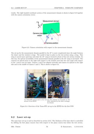
93. 6.2. LASER SET-UP CHAPTER 6. TOMO-PIV CAMPAIGN
Table 6.2: Geometrical characteristics of the measurement set-up parallel to the 45◦
ramp
ϕ[◦
] θ[◦
] ω[◦
] distance in z[mm]
Camera 1 −40 −31 30 426
Camera 2 −1 −44 26 408
Camera 3 −9 −19 23 430
During the current experiments, a laser sheet thickness of approximately 6 mm is wanted. Furthermore,
a relative small velocity in wall-normal direction is expected compared to the high convective stream-
wise velocity. Therefore, the time interval (∆t) between the two laser pulses and camera snap shots is
increased to∆ t = 2µs. The particle displacement in z direction is increased which is often referred to
as an increase in dynamic range. In figure 6.5(a) and 6.5(b) the laser sheet alignment with respect the
model for both both FOVs is given. In figure 6.5(c) and 6.5(d), the illuminated domain is indicated in
the corresponding Schlieren image for Re = 14.1 × 106
m−1
and hzz = 1.15mm.
(a) The laser set-up parallel to the 5◦ ramp (b) The laser set-up parallel to the 45◦ ramp
(c) The illuminated domain indicated in the
Schlieren image for the case that Re = 14.1 ×
106m−1 and hzz = 1.15mm
(d) The illuminated domain indicated in the
Schlieren image for the case that Re = 14.1 ×
106m−1 and hzz = 1.15mm
Figure 6.5: Laser sheet orientation for both measurements parallel to first and parallel to the 45◦
ramp
Based on the Schlieren image given in figure 6.5(c), it is expected to see the influence of the separation
shock parallel to the 5◦
. At the 45◦
ramp there are expansion waves and shocks impinging on the surface
of the wall and wave reflection takes place. Based on figure 6.5(d), it expected to see the influence of the
reattachment shock and an expansion wave that originates from the shock interaction above the 45◦
ramp.
For both measurement volumes, the spacing between the laser sheet and the surface of the model is
set at 2mm. The laser sheet thickness is checked by looking at the mean particle intensity per plane in
the reconstructed data. During the self-calibration, the laser sheet thickness is roughly determined based
on the appearance of peaks in the z-plane. The self-calibration is applied and the particle distribution is
reconstructed for the measurement domain and a large domain outside of the illuminated volume. This
procedure gives the following information:
• Distance between the laser sheet and the model surface
• Laser sheet thickness
MSc. Thesis 77 D. Ekelschot, 1 2 6 6 3 0 6

94. 6.3. REFRACTIVE EFFECT CHAPTER 6. TOMO-PIV CAMPAIGN
• Estimate of the ghost particle intensity
In figure 6.6 the mean intensity is plotted in z-direction. the coordinate system is right handed and
therefore the z-axis is positive pointing away from the model. The position of z = 0 varies per new
calibration procedure.
−6 −4 −2 0 2 4 6
800
850
900
950
1000
1050
1100
z [mm]
Imean
[counts]
(a) The mean intensity plotted in z direction for
the measurement domain parallel to the 5◦ ramp
−8 −6 −4 −2 0 2 4
100
150
200
250
z [mm]
Imean
[counts]
(b) The mean intensity plotted in z direction for
the measurement domain parallel to the 45◦ ramp
Figure 6.6: The mean Intensity plotted in z direction to check the sheet thickness
The red lines shown in figure 6.6(a) and 6.6(b) indicate the estimated location of the laser sheet edges
based on the self-calibration procedure. The blue line indicates a significant increase in intensity level
due to the laser light. It is concluded that for both FOVs, the estimated sheet thickness based on the
self-calibration corresponds with the reconstructed thickness.
The reconstruction treats the reflections of the model as illuminated particles which are fixed in space.
The peaks in negative z direction with respect to the laser sheet, shown in figure 6.6(a) and 6.6(b),
represent the position of the model. For both measurement volumes, the distance with respect to model
is approximately 2.2mm.
6.3 Refractive effect
Light refraction has to be taken into account when an optical flow measurement technique is used in
a pressurised test facility such as the HTFD. Vacuum conditions are present in the test section and
consequently, a difference in density between the ambient and the test section is present. As a result,
the refractive index changes which influences in particular optical measurement techniques that require
highly accurate calibration procedure such as Tomo-PIV.
During the initial test phase it was noticed that the particle triangulation during the self-calibration
procedure is significantly influenced when particle images are taken in ambient conditions. This can be
ascribed to the light refraction that occurs during the measurement. As a result, it is chosen to collect
typically 30 images more after the run such that a summed disparity map over these 30 images can
be obtained. The influence of the number of calibration images on the quality of the disparity map is
elaborated in section 3.4.1. Directly after the run, the pressure is then still significantly low and therefore
a self-calibration is performed on the residual images of the run to compensate for refractive effects. This
section serves as a validation and indication of the relevance of the refractive effect during a Tomo-PIV
experiment in the HTFD.
From refractive theory it is known that the refractive index is linearly dependent on the density of
the medium. Mathematically, this is described using the Gadstone-Dale relation.
n = 1 + kρ (6.5)
where n is the refractive index, k = 2 × 10−4
and ρ is the density. The analogy presented in this section
relies on the pointing of a single pixel and therefore the pixel shift is considered to be the error in the
MSc. Thesis 78 D. Ekelschot, 1 2 6 6 3 0 6

95. 6.3. REFRACTIVE EFFECT CHAPTER 6. TOMO-PIV CAMPAIGN
pointing of the cameras.
Snell’s law is used to determined the pixel offset induced by light refraction.
θ
= arcsin
sin(θ)n1
n2
(6.6)
In figure 6.7(a) a sketch is given of one camera with its corresponding pointing error dpix due to the
pressure difference between the test section and the ambient surroundings.
(a) Sketch of the refractive effect and the corre-
sponding pixel shift
(b) Sketch of the incoming light ray (blue), the re-
fractive interface (window) and the refracted light
ray (red) with the corresponding angles
Figure 6.7: Graphical representation of the refractive effect
The refractive effect for a three-camera set-up is worked out for the camera set-up parallel to the 5◦
ramp.
It is assumed that the distance between the image and the object plane are the same (z = 400mm) for all
cameras. Furthermore it is assumed that the window is in the middle between the image and the object
plane. In figure 6.7(b) a sketch is given of a incoming light ray (blue arrow) together with the refractive
interface (window) and the refracted light ray (red arrow). The light ray is refracted in two directions
indicated by the angles θ and ϕ. Snell’s law (see equation 6.6) is used to obtain the two relevant refraction
angles for the lines of sight for all three cameras.
The error is determined and a graphical representation is given in figure 6.8.
The coloured dots represent the three different cameras (camera 1 red, camera 2 mangenta and camera 3
green). The blue lines represent the lines of sight for every camera for the case that there is no pressure
difference between the test section and the ambient. The green lines that start from the refractive inter-
face (window is represented by the black dots), represent the light refracted when it passes the refractive
interface.
Snell’s law states that light refracts further away from the normal since the density is lower behind
the interface. As a result of the refracted light beam, it can be seen that the three cameras are not
pointing in the same direction but they span a triangular two dimensional plane which represents the
pointing error for this particular three-camera set-up. Note that the case presented in figure 6.8 is not
physical since the pixel shift for each camera is in the order of 1 pixel rather than 10 mm as given in
figure 6.8.
The norm is taken for the individual cameras and given in table 6.3. Based on table 6.3, the relative
pixel shift is in the order of 1 pixel.
MSc. Thesis 79 D. Ekelschot, 1 2 6 6 3 0 6

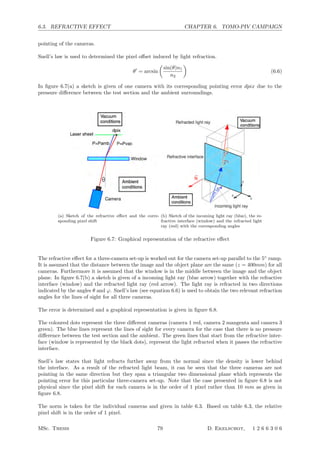
96. 6.3. REFRACTIVE EFFECT CHAPTER 6. TOMO-PIV CAMPAIGN
−200
−150
−100
−50
0
50
100
0
50
100
150
200
250
300
350
400
−20
0
20
40
60
80
100
120
x [mm]
θ
1
=−30φ
1
=3,θ
2
=−7,φ
2
=−17,θ
3
=15,φ
3
=3
z [mm]
y[mm]
Figure 6.8: Three dimensional theoretical error estimation due to the refractive effect
Table 6.3: Pixel shift
Camera1 Camera2 Camera3
∆pix ±0.75pix ±0.3pix ±0.4pix
The pixel shift is determined experimentally by taking an image of a Lavision type 10 calibration plate
at 6 different a test section conditions. An image is taken at ambient pressure. The vacuum tank is
switched on and images are taken at p = 476 mbar, p = 171 mbar, p = 80 mbar, p = 27 mbar and p = 1
mbar. The images taken at lower pressure are then cross-correlated with the image taken at ambient
pressure. In this way, the pixel shift for all three cameras are determined. In figure 6.9, the disparity
map is given for the three camera set-up used to measure the velocity field parallel to the 5◦
ramp.
−4 −3.5 −3 −2.5 −2 −1.5 −1 −0.5 0
−0.8
−0.6
−0.4
−0.2
0
0.2
0.4
0.6
0.8
∆ x
pix
∆y
pix
Camera 1
Camera 2
Camera 3
Pvac = 476 mbar
Pvac = 171 mbar
Pvac = 80 mbar
Pvac = 27 mbar
Pvac = 1 mbar
(a) The experimentally determined pixel shift for the three
camera set-up used for FOV 1
−0.495 −0.494 −0.493 −0.492 −0.491 −0.49 −0.489 −0.488
−0.525
−0.52
−0.515
−0.51
−0.505
−0.5
−0.495
−0.49
∆ x
pix
∆y
pix
Camera 2
Camera 3
Pvac = 1 mbar
Pvac = 27 mbar
Pvac = 80 mbar
Pvac = 171 mbar
Pvac = 476 mbar
Pvac = 476 mbar
Pvac = 80 mbar
Pvac = 171 mbar
Pvac = 1 mbar
Pvac = 27 mbar
(b) Detail of the experimentally determined pixel shift for
camera 2 and 3
Figure 6.9: Experimentally determined pixel shift for the three camera set-up used for FOV 1
Note, that the pixel shift of camera 1 is in the order of 2 to 3 pixels while for camera 2 and 3 the pixel shift
is significantly lower (0.5 pixel). Furthermore, it is observed that for camera 1 the pixel shift becomes
larger when the pressure drops which is also expected from theory. However, this is not the case for
camera 2 and 3 shown in figure 6.9(b).
Note, that the pixel shift is in negative direction for all three cameras. From theory, it was expected,
MSc. Thesis 80 D. Ekelschot, 1 2 6 6 3 0 6

97. 6.3. REFRACTIVE EFFECT CHAPTER 6. TOMO-PIV CAMPAIGN
that refraction takes place in opposite direction for the opposite cameras (see camera 1 (red) and camera
3 (green) in figure 6.8). The large overall pixel shift might be due to the fact that the window tilts
with respect to the image plane due to the pressure difference between the ambient conditions outside
and the vacuum conditions inside the test section. A tilted refractive interface results in an overall pixel
shift in one direction (depending on the tilt angle) for opposite viewing angles. The pixel shift obtained
experimentally, is in negative direction for all three cameras. Therefore, a tilted refractive index might be
the cause of this and therefore this is further investigated. A graphical representation is given in figure
6.10.
(a) Refractive effect without a titled
window
(b) Refractive effect with a titled win-
dow
Figure 6.10: Graphical representation of the pixel shift caused by a tilted refractive interface
The orange arrow indicates the propagation direction of the light ray when the test section would be
at ambient pressure. The red arrow indicates the refracted light ray. On the right hand side, a similar
sketch is given but now the refractive interface is tilted. The angle θ
1 can be defined in terms of a:
θ
1 = θ1 + a (6.7)
Using Snell’s law, the refracted angle θ
2 becomes:
θ
2 = arcsin
sin (θ + a)n2
n1
(6.8)
The refracted angle, θ
2, can then be written in terms of the original coordinate system:
θ2,new = θ
2 − a = arcsin
sin (θ + a)n2
n1
− a (6.9)
The pixel shift due to the tilted window can be written as:
dpixa = sin(θ2) · l − sin(θ2,new) · l (6.10)
where l is the distance between the refractive interface and the object. The theoretical pixel shift dpixa
is plotted against the viewing angle (θ1) and different tilt angles (a) of the refractive interface in figure
6.11(a). To see the direct influence of the tilt in refractive index, the refractive effect present for a aligned
MSc. Thesis 81 D. Ekelschot, 1 2 6 6 3 0 6

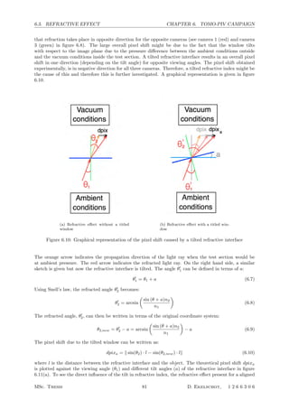
98. 6.4. SELF-CALIBRATION CHAPTER 6. TOMO-PIV CAMPAIGN
θ [deg]
a[deg]
−40 −20 0 20 40
−5
0
5
dpix
−2
−1
0
1
2
(a) The total pixel displacement plotted against de
viewing angle (θ) and the tilt angle of the window
(a)
θ [deg]
a[deg]
−40 −20 0 20 40
−5
0
5
dpix
a
−0.6
−0.4
−0.2
0
0.2
0.4
0.6
(b) The pixel shift solely induced by the tilt angle
(a), plotted against the viewing angle (θ) and the
tilt angle of the window
Figure 6.11: Pixel shift induced by the tilting of the window
refractive index has to be subtracted (dpixa − dpix). This is plotted in figure 6.11(b).
Figure 6.11(b) confirms that a positively tilted window, refracts the light more positively for both a cam-
era with a positive and a camera with a negative viewing angle. Hence, this could explain why the pixel
shift found during the experimental analysis are all in the same direction. A tilted refracted interface can
therefore be considered as the cause of the discrepancy found between the theoretical analysis shown in
figure 6.8, and the experimental analysis shown in figure 6.9.
Furthermore, it can be concluded, that the absolute pixel shift solely induced by the tilting angle of
the window, does not correspond with the large pixel displacement obtained during the experimental
analysis (at least 0.5 pixel). However, during the theoretical analysis as shown above, only one direction
is taken into account. Nevertheless, this effect occurs in two directions as shown in figure 6.7(b).
6.4 Self-calibration
As shown in the previous section, the line of sight of each camera is influenced by the pressure difference
between the test section and the ambient surrounding. Based on the 2D images from the different view-
ing angles, a particle triangulation procedure is performed and the disparity with respect to the plate
calibration is determined (see section 3.4.1). The calibration function is updated based on the disparity
map. One needs to make sure that the disparity map is calculated under similar conditions as present
during the measurement. Therefore, it is not possible to perform a self-calibration procedure at ambient
conditions since the lines of sight will differ when the pressure in the test section decreases (see previous
section). Consequently, the self-calibration is performed based on the extra images that are taken after
the run. The particle density in these images is sufficient and the pressure in the test section while taking
these images is nearly similar to the pressure during the run.
The self-calibration procedure improves the plate calibration. The plate calibration is rather rough
since it is based on one plate position and thus two z-positions. As a result, the third order polynomial
is rather inaccurate due to the limited amount of fitting points. A typical fit rms is found in the order
of 0.2 pix. The Lavision Type 10 calibration plate has a 10 mm spacing between the dots. Local posi-
tions in between the dots in the measurement domain are determined using bilinear interpolation. The
measurement domain has the following dimensions:
(xvol, yvol, zvol) = (60mm, 40mm, 6mm)
The voxel distribution within the measurement domain for both FOVs is given in table 6.4 The volume is
split up in sub-volumes to refine the set of calibration data points. The definition and typical values for
a sub-volume size, threshold value and search radius were introduced in section 3.4.1. The measurement
volume is split up in (nx × ny × nz = 6 × 6 × 5 = 10 mm × 6.7 mm × 1.2 mm) sub-volumes where the
MSc. Thesis 82 D. Ekelschot, 1 2 6 6 3 0 6

99. 6.5. INTERROGATION VOLUME SIZE CHAPTER 6. TOMO-PIV CAMPAIGN
Table 6.4: Geometrical characteristics of the measurement set-up parallel to the 5◦
ramp
voxx[−] voxy[−] voxz[−]
FOV parallel to 5◦
ramp 1300 940 140
FOV parallel to 45◦
ramp 1420 980 120
local disparity vector is determined based on particle triangulation. The threshold value (T = 150 − 200
counts depending on the average particle intensity) is set such that the particle triangulation lies below
10000 (rule of thumb) for all the three cameras. The search radius is initially set to = 4. After refine-
ment (nx × ny × nz = 9 × 9 × 8 = 6.7 mm× 4.44 mm × 0.75 mm) , = 0.5 and T = 100 − 150), the
self-calibration is performed again and the peak displacement is reduced in the order of d = O(10−3
). The
calibration function is refined by taking a larger number of sub-volumes since the third order polynomial
is fit through more points.
In Appendix D, the disparity maps are given for two iteration steps for both FOVs. It is forced by
geometrical limitations of the test section to place the calibration in a rotated position for the measure-
ment domain parallel to the 45◦
ramp. This can be seen in the self-calibration images, since no signal is
present in upper right and lower left corner (see figure D.1(c)). In figure D.1(c) can be seen that a high
amount of particle triangulations is found in the lower right corner due to local reflection of the laser
light on the model. It is made sure that no spurious vectors are present. After a vector smoothening
procedure, the calibration file is updated. Finally the fit rms of the third order polynomial is reduced to
O(10−3
).
6.5 Interrogation volume size
In section 3.3, the importance of the ppp during a 2C-PIV experiment is emphasised. An estimate of
the Particles Per Voxel (ppv) is presented based on the 2D raw images. A function is written in Matlab
which determines the local maxima in the image. The user gives in a threshold value and a search radius.
The threshold is based on a priori investigation of the raw image, hence the user finds an estimate of
the particle pixel intensity. The search radius is dependent on the size of the particles. In figure 6.12 a
sample of an image is given with a zoomed-in view of the particle intensity map highlighted by the red
lines in figure 6.12(a). The red dots in figure 6.12(b) represent points which are counted as particles by
the Matlab script.
(a) Sample image from which the ppp is determined (b) Zoomed in on the sample image to indicate the
particle detection
Figure 6.12: Determination of the ppp
The ppp is estimated to be 0.018. Based on this number the correlation volume size is determined. Again
MSc. Thesis 83 D. Ekelschot, 1 2 6 6 3 0 6

100. 6.6. SPURIOUS VECTOR DETERMINATION CHAPTER 6. TOMO-PIV CAMPAIGN
it is assumed to have 9 particle pairs per volume to obtain a qualitative correlation peak. Assuming a
cubic correlation volume this results in a interrogation volume of the following size:
9
w3
=
ppp
zvox
→ w = 3
9
ppp
zvox
= 3
9
0.018
120
≈ 45pix (6.11)
The longitudinal vortical structures are identified by the rotational flow behaviour in the (y, z) plane
and hence it is wanted to have a high spatial resolution in y and z. Therefore, the correlation volumes
are elongated in x direction such that the spanwise and normal width of the correlation volume can be
decreased. During the 3D cross-correlation procedure, a correlation volume of 65 × 56 × 32 voxels is used
which corresponds to 3.2 mm × 2.8 mm × 1.6 mm. Typically 120 voxels in z-direction are taken such
that with an overlap of 75% approximately 15-20 vectors are found in normal direction. An estimate of
the amount of vectors per mm is given in the table below:
Table 6.5: Number of vectors
x y z
vec/mm 3.33 2.5 3.33
6.6 Spurious vector determination
For both FOVs typically 20-30 runs are taken to obtain a statistical average. Spurious vectors occur due
to low local particle density, bad flow conditions, bad windtunnel/acquisition timing or flaws during the
data analysis procedure. These vectors have to be accounted for to obtain a plausible average velocity
field. A local statistical procedure is performed based on the number of runs. Initially, the standard
deviation at every local point in the measurement domain is determined in the following way:
¯σi =
1
Nr
Nr
i=1
(ui − ¯ui)
2
(6.12)
where Nr is the number of runs, ui = [Vx, Vy, Vz] and ¯ui = [ ¯Vx, ¯Vy, ¯Vz] is the mean velocity. Consider the
local measurement data to be normally distributed. Hence, a local velocity measurements should fulfill
the following relation to be considered as valid.
¯ui − 3σ ≤ ui ≤ ¯ui + 3σ (6.13)
When the vector is considered to be spurious, it is replaced by the new mean value based on the other
corresponding local data points. From this point on, a new standard deviation value is determined based
on the replaced vectors. This procedure is iterated until no more spurious vectors are replaced.
6.7 Accuracy estimation
Little is known regarding the error estimation of a Tomo-PIV experiments due to the complexity of the
technique. The accuracy of the measurement is therefore estimated by applying the appropriate statisti-
cal analysis for a case of known flow conditions. Hence, the relative fluctuations for a steady, undisturbed,
uniform flow situation are determined.
As a case study for the measurement domain parallel to the 5◦
ramp, a validation run is taken dur-
ing which the model is removed from the test section. The particle density is uniform since no shocks
are present. It is expected to have a high streamwise velocity (Vx ≈ cos(5) × 1033 = 1021m/s) and a
slightly diverging Vy. Since the light sheet is already positioned parallel to 5◦
ramp, it is expected to
have a negative Vz component since the flow is aligned with the longitudinal wind tunnel axis instead of
the 5◦
inclined model surface such that Vz = sin(5) × 1033 ≈ 90m/s.
The standard deviation in the (y, z) plane is of interest since the flow rotation in this plane is fur-
ther studied. Therefore, the standard deviation in each (y1, z1) plane is determined for the case that no
MSc. Thesis 84 D. Ekelschot, 1 2 6 6 3 0 6

101. 6.7. ACCURACY ESTIMATION CHAPTER 6. TOMO-PIV CAMPAIGN
model is present and the unit Reynolds number is equal to Re = 14.1 × 106
[m−1
]. In figure 6.13(a),
the in-plane mean velocity component is plotted in x1 direction and in 6.13(b) the in-plane standard
deviation of Vx, Vy and Vz is plotted in x1 direction.
−20 −10 0 10 20 30
−1200
−1000
−800
−600
−400
−200
0
x [mm]
σ[m/s]
Vx
Vy
Vz
(a) Mean Vx Vy and Vz in the (y, z) plane plotted in x di-
rection for the velocity field parallel to the 5◦ ramp
−20 −10 0 10 20 30
0
5
10
15
20
25
x [mm]
σ[m/s]
Vx
Vy
Vz
(b) The (y, z) plane rms values for all the velocity compo-
nents plotted in x direction for the velocity field parallel to
the 5◦ ramp
Figure 6.13: Measurement accuracy assessment for FOV 1
Table 6.6: Standard deviation and mean for every velocity component in the (y1, z1) plane for the
presented test case
std[m/s] mean[m/s] std[%]
Vx 0.56 1008 0.056
Vy 6.2 77.5 8.0
Vz 17.4 109.7 15.9
It is found that the standard deviation for Vz is significantly higher (approximately a factor 3) than for
Vx and Vy. Fluctuations that exceed this percentage are impossible to measure in a single instantaneous
(y1, z1) plane based on the presented case study.
During the measurement campaign for the measurement domain parallel to the 45◦
ramp, a valida-
tion run is taken during which the model is still present in the test section. For this case, the model is
present in the test section but it is moved away from the window (in spanwise direction of the windtunnel)
such that the distance between the model and the laser sheet becomes approximately 25 mm. In this
way, the local free stream velocity is obtained. It is noted that the bow shock is present such that only
a small portion of the free stream flow domain is captured. A similar procedure is then performed as
described for the FOV parallel to the 5◦
ramp. The free stream flow parallel to the model is measured
and it is made sure that no fluctuations are present in the flow. The mean of all velocity components in
the (y2, z2) plane is plotted in x2 direction in figure 6.14(a) and the corresponding standard deviation is
given in 6.14(b).
Due to the shock, two velocity field are present governed by their convective velocity Vx. This effects
the standard deviation in the (y, z) plane and therefore both cases are presented in table 6.7 separately.
Again a high standard deviation for Vz is found especially upstream of the shock which indicates that
the flow is not uniform since the standard deviation for Vz downstream of the shock is significantly lower
and of the same order as the standard deviation in Vy. With respect to the mean corresponding velocity
component, the standard deviation of Vz is very large. This gives an indication of the range of velocities
that can be measured in x, y and z direction.
MSc. Thesis 85 D. Ekelschot, 1 2 6 6 3 0 6

102. 6.7. ACCURACY ESTIMATION CHAPTER 6. TOMO-PIV CAMPAIGN
−70 −60 −50 −40 −30 −20
−1000
−800
−600
−400
−200
0
200
400
600
x [mm]
Vmean
[m/s]
Vx
V
y
Vz
(a) Mean Vx Vy and Vz in the (y, z) plane plotted in x di-
rection for the velocity field parallel to the 45◦ ramp
−70 −60 −50 −40 −30 −20
0
50
100
150
200
x [mm]
σ[m/s]
Vx
V
y
Vz
(b) The (y, z) plane rms values for all the velocity compo-
nents plotted in x direction for the velocity field parallel to
the 45◦ ramp
Figure 6.14: Measurement accuracy assessment for FOV 2
Table 6.7: Standard deviation and mean for every velocity component in the (y, z) plane for the presented
test case
Upstream of the shock Downstream of the shock
mean[m/s] std[m/s] std[%] mean[m/s] std[m/s] std[%]
Vx −441 26.5 6 963 59 6
Vy 177 16.3 9.2 385 38 10
Vz −2.9 16.3 565 −41 45 110
MSc. Thesis 86 D. Ekelschot, 1 2 6 6 3 0 6

103. 6.8. RECONSTRUCTION QUALITY ESTIMATION CHAPTER 6. TOMO-PIV CAMPAIGN
In general it can be stated that the pixel displacement in x and y direction are considered to be large
enough to measure the local velocity. Unfortunately, the convective velocity in z direction is low and the
dt is small (dt = 2µs, see section 6.2). The short∆ t therefore limits the dynamic range in z direction.
This effect becomes even worse if the particles are stretched in z direction as well. For now, this is
considered to be the reason for the high noise level in the Vz determination. Consider that Vz = 20 m/s
and estimating the magnification to be M = 1376/0.06 = 2.3 × 104
then:
∆pix,z = Vz · M · ∆t = 20 · 2.3 × 104
· 2 × 10−6
= 0.92pixel (6.14)
The displacement in z direction is in the order of the radius of the particle.
6.8 Reconstruction quality estimation
An indication of the particle shaped is obtained by analysing the reconstructed particle distribution. The
particle distribution is saved as a -ascii from Davis 7.4 and read into Matlab. The data set consists of
voxz planes with each having a size of voxx × voxy. Using a 2D correlation procedure, an estimate of the
pixel shape is determined. The correlation factor in z direction is determined using:
R(z) =
x
y I(x, y, z) ⊗ I(x, y, z + ∆z)
x
y I(x, y, z)2
(6.15)
For a fixed z position, typically 10 planes in normal direction are correlated to investigate the shape
of the reconstructed particles in this particular direction. This procedure is also performed for x and
y direction. Based on priori investigation of the reconstructed data, it is determined that the particle
images in the (x, y) look Gaussian shaped. Furthermore, this procedure is performed at several locations
in the measurement and the mean of each individual correlation signal is obtained. The results for both
the measurement domain parallel to the 5◦
and the 45◦
ramp are shown in figure 6.15(a) and 6.15(b)
respectively.
0 2 4 6 8 10
0
0.2
0.4
0.6
0.8
1
vox [#]
R[−]
Rx
R
y
Rz
(a) Correlation factor in x, y and z for the measurement
domain parallel to the 5◦ ramp
0 2 4 6 8 10
0
0.2
0.4
0.6
0.8
1
vox [#]
R[−]
Rx
R
y
Rz
(b) Correlation factor in x, y and z for the measurement
domain parallel to the 45◦ ramp
Figure 6.15: Correlation factor in x, y, z based on the reconstructed particle distribution
From figure 6.15(a) can be seen that the correlation factor in x and in y direction are nearly similar.
During the observation of the reconstruction image, it was determined that the pixels looked round and
not stretched. The result shown in figure 6.15(a) therefore corresponds to this observation. However, for
the correlation factor in z direction, it can be seen that it takes a larger amount of voxels in z direction
to have uncorrelated image planes. This indicates that the size of the particles is stretched in z direction.
Similar results are shown for the FOV parallel to the 45◦
in figure 6.15(b). However, it is observed,
that there is a discrepancy present between Rx and Ry. which indicates that the particles are not com-
pletely round but slightly stretched in y direction. Again an offset for Rz with respect to Rx and Ry
MSc. Thesis 87 D. Ekelschot, 1 2 6 6 3 0 6

104. 6.9. GENERAL FLOW TOPOLOGY CHAPTER 6. TOMO-PIV CAMPAIGN
is observed which indicates that the particles are stretched in z direction as well. This will widen the
correlation peak significantly and cause an uncertainty that might be in the order of the value that is
given in equation 6.14.
6.9 General flow topology
In figure 6.16 an overview of the flow is given. For interpretation purposes, it is decided to show first the
general flow overview. In section 6.10 and 6.11 the individual velocity fields are discussed in more detail.
The outline of the surface of the model is indicated by the thick black lines. The velocity field behind the
leading edge shock is indicated by orange (Vtot ≈ 1000 m/s) corresponds with the values found during
the planar PIV campaign and theory, shown in chapter 4. The flow is then rapidly decelerated by the
separation shock at x ≈ 15mm. The flow is curved upwards which is indicated by the streamlines in the
following section. The flow reattaches at the 45◦
ramp and the velocity is increased by a Prandtl-Meyer
expansion fan that emanates from the shock interaction above the surface of the model. This is indicated
by the green domain parallel to the 45◦
ramp where the flow is accelerated from 450m/s up to locally
750m/s. The flow is then compressed and slowed down to approximately 550m/s after which again a
graduate acceleration takes place up to approximately 675m/s.
Figure 6.16: General 3D flow overview
In figure 6.17 an iso-surface plot is given of the total velocity. Note longitudinal iso-surfaces for Vtot = 990
m/s parallel to the 5◦
ramp. The velocity decreases due to the separation shock at x ≈ 15 mm. Note the
isoplanes in normal direction with respect to the surface of the model at x ≈ 20 mm and at x ≈ −10 mm.
The separation and reattachment shock are present at these streamwise locations respectively. Further-
more, note the locally high velocity regime (Vtot ≈ 750 m/s) parallel to the second ramp corresponding
to the local high ch domains determined using QIRT (see chapter 5). The characteristic local velocity
fields are discussed in detail in the following sections.
MSc. Thesis 88 D. Ekelschot, 1 2 6 6 3 0 6

105. 6.10. FLOW TOPOLOGY 5◦
RAMP CHAPTER 6. TOMO-PIV CAMPAIGN
Figure 6.17: General 3D flow overview
6.10 Flow topology parallel to the 5◦
ramp
Parallel to the 5◦
ramp, it is expected to have a upstream velocity equal to the velocity determined behind
the leading edge shock using 2C-PIV. Furthermore, the separation shock and the separated flow domain
just upstream of the first-to-second ramp junction of the model is expected. The QIRT measurements
indicated that the size of the separation bubble decreases for higher VGs and separation takes place at
approximately x = 20 mm based on the QIRT results presented in chapter 5. A flow overview is given
in figure 6.18 where the contours of the total velocity is plotted together with a rake of streamlines. The
influence of the separation shock on the velocity is clearly visualised in the (x, z) planes. In this section
the coordinate system (x1, y1, z1) is used, as indicated in figure 6, and referred to as (x, y, z) such that
x is tangent to the 5◦
ramp, y the spanwise coordinate and z the normal coordinate, positive pointing
away from the model.
The velocity field shown in figure 6.18 corresponds with the Schlieren image given in figure 6.5(c). At
approximately 20 mm, the flow separates and a free stream velocity field is measured upstream of the
separation line. Furthermore, the flow will slow down near the deflection point and no back flow is present
which is shown in figure 6.19.
In figure 6.19 the mean streamwise velocity profile is given. it can be seen that velocity measured upstream
of the shock is slightly below the value which is found using the oblique shock relations (Vtot = 1015
m/s). This is caused by the extra shock wave that emanates from the VG. The planar PIV results show a
local velocity of 1020 m/s. The gradient near the deflection point induced by the separation shock is high
since the velocity in streamwise direction decreases from 900 m/s to 200 m/s over 15 mm. In contrast
to the planar PIV experiments carried out for the case hzz = 0, there is no circulation bubble and thus
no back flow present. In figure 6.20 the normal velocity component (Vz) is plotted in the (x, z) plane.
This velocity component is approximately 1% of Vx and the gradient in z-direction is relatively small.
This indicates that the flow is not smoothly curved upwards but a radical velocity change is present. Vz
increases away from the model surface which lies within the expectations.
MSc. Thesis 89 D. Ekelschot, 1 2 6 6 3 0 6

106. 6.10. FLOW TOPOLOGY 5◦
RAMP CHAPTER 6. TOMO-PIV CAMPAIGN
Figure 6.18: Flow overview parallel to the 5◦
ramp. Velocity magnitude is given in m/s
Figure 6.19: Contour map Vx parallel to the 5◦
ramp
Figure 6.20: Contour map Vz parallel to the 5◦
ramp
MSc. Thesis 90 D. Ekelschot, 1 2 6 6 3 0 6

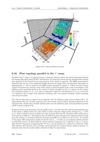
107. 6.10. FLOW TOPOLOGY 5◦
RAMP CHAPTER 6. TOMO-PIV CAMPAIGN
The VG introduces a spanwise perturbation in the near-wall flow regime. Therefore, the spanwise ve-
locity field is further investigated. To identify perturbations in the flow, the data is filtered using a
Savitzky-Golay smoothing filter which is often used in the field of noisy signal processing Savitzky and
Golay [1964]. The perturbations induced by the VG are very small compared to the convective velocities
in particular Vx and Vy. The main goal is to relate the longitudinal heat flux streaks to the velocity
profile measured using Tomo-PIV. Longitudinal vortices are expected and therefore the v
y and v
z profile
is expected in the spanwise direction given in figure 4.18. On the left hand side of figure 6.21, the span-
wise Vy and Vz distribution is given for four fixed x positions. On the right hand side, the corresponding
filtered spanwise v
x, v
y and v
z distribution is given.
−20 −10 0 10 20
−5
0
5
10
15
20
Spanwise velocity fluctuations at x =51.4
y [mm]
v[m/s]
V
y
V
z
(a) Vy and Vz distribution in the middle of (y,z)
plane at x = 51.4mm
−20 −10 0 10 20
−5
0
5
Spanwise velocity fluctuations at x =51.4
y [mm]
v[m/s]
v
x
v
y
vz
(b) Perturbations v
y and v
z distribution in the mid-
dle of (y,z) plane at x = 51.4mm
−20 −10 0 10 20
−5
0
5
10
15
20
25
Spanwise velocity fluctuations at x =45.5
y [mm]
v[m/s]
V
y
V
z
(c) Vy and Vz distribution in the middle of (y,z)
plane at x = 45.5mm
−20 −10 0 10 20
−6
−4
−2
0
2
4
Spanwise velocity fluctuations at x =45.5
y [mm]
v[m/s]
v
x
v
y
vz
(d) Perturbations v
y and v
z distribution in the mid-
dle of (y,z) plane at x = 45.5mm
−20 −10 0 10 20
−5
0
5
10
15
20
25
Spanwise velocity fluctuations at x =30.72
y [mm]
v[m/s]
V
y
V
z
(e) Vy and Vz distribution in the middle of (y,z)
plane at x = 30.72mm
−20 −10 0 10 20
−8
−6
−4
−2
0
2
4
6
Spanwise velocity fluctuations at x =30.72
y [mm]
v[m/s]
v
x
v
y
vz
(f) Perturbations v
y and v
z distribution in the mid-
dle of (y,z) plane at x = 30.72mm
Figure 6.21: The spanwise v
y and v
z distribution for four fixed x positions
During the data analysis, it has been noticed that the influence of the VG on the velocity field is relative
MSc. Thesis 91 D. Ekelschot, 1 2 6 6 3 0 6

108. 6.11. FLOW TOPOLOGY 45◦
RAMP CHAPTER 6. TOMO-PIV CAMPAIGN
small compared to the convective speed Vx. By specifying the range of interest to 980 ≤ Vx ≤ 1005 m/s,
clear fluctuations are visualised which are induced by the VG. The spanwise Vx and v
y distributions at
four fixed x positions are plotted in figure 6.22.
For every fixed x position, the 10 upstream and 10 downstream spanwise velocity profiles are taken and
the mean is calculated. This corresponds with taking the average over a range of approximately 6 mm
in streamwise direction.
It can be seen that clear velocity fluctuations are present which correspond with the wavelength of
the VG (λV G = 6mm). The gradient is relatively low which can be seen by the contour values indicated
in figure 6.22. The difference between the higher and lower velocity regions is approximately 10 m/s
while the total velocity is in the order of 1000 m/s.
The standard deviation of Vx is determined based on the individual snap shots. The spanwise Vx distri-
bution is given together with the corresponding contour plot of the standard deviation in Appendix E.
Based on this figure, it can be seen that the position of the longitudinal streaks is rather fixed and within
each streak, no velocity fluctuations are present. This indicates that the streaks are not turbulent.
The v
y and v
z vectors do not show clear vortical behaviour. Within the measurement domain paral-
lel to the 5◦
ramp, the influence of the VG is clearly noticed on the streamwise and spanwise velocity
component. However, not a clear fluctuating behaviour of Vz is noticed which would be expected when
having longitudinal vortices. This is due to the fact that v
z are expected to be of the same order as v
y
(O(1m/s)). The high rms value in Vz does not allow an accurate measurement of such small spanwise
fluctuations as shown in the previous section.
The correlation of Vx and v
y show a similar pattern that is found by Sch¨ulein and Trofimov [2011].
A higher Vx domain is measured at spanwise position where the perturbation vectors point towards each
other and a lower local Vx domain is measured where the perturbation vectors are pointing away from
each other. This corresponds to what is presented in figure 4.22(a) Sch¨ulein and Trofimov [2011]. This
follows as well from the perturbation plots given in figure 6.22. The velocity fluctuations,v
x and v
y are
slightly out of phase which is expected based on the image given in figure 4.22(a).
6.11 Flow topology parallel to the 45◦
ramp
A similar flow description is given for the velocity field parallel to the 45◦
. During this discussion, the
coordinates (x2, y2, z2) given in figure 6 are referred to as (x, y, z) such that x is tangent to the 45◦
ramp,
y the spanwise coordinate and z the normal coordinate, positive pointing away from the model.
During the calibration phase it is noted that the calibration could not be properly aligned with the
surface of the 45◦
ramp. Therefore the calibration plate is rotated around the z-axis. The rotation
angle, ω = 22◦
is determined during the self-calibration phase and checked with the extra runs taken for
measurement validation. The velocity components and the (x, y) domain are therefore rotated to obtain
the correct velocity components parallel to the 45◦
ramp.
The measurement domain is defined 2.2 mm away from the surface of the 45◦
ramp. In figure 6.23
the contour plot of the total velocity together with the corresponding streamlines are given within the
3D measurement domain.
The streamlines at reattachment indicate a typical pattern of cropped streamlines that diverge and
progress into straight longitudinal streaks. This is also found by Sch¨ulein and Trofimov [2011] using
oil flow visualisation (see figure 4.22(b)). Furthermore, a local low velocity domain near reattachment
is observed upstream at x = −15 mm. The primary features of the flow parallel to the 45◦
ramp are
discussed by looking at the streamwise development of the velocity field. The spanwise mean of Vx is
plotted in x direction as shown in figure 6.24.
The Vx streamwise distribution indicates velocity drop near the first the second ramp junction due to
the reattachment shock at x −15mm. Locally, the velocity parallel to the 45◦
ramp increases at
x ≈ −30mm. This can be ascribed to the expansion wave which originate from the shock interaction
MSc. Thesis 92 D. Ekelschot, 1 2 6 6 3 0 6

109. 6.11. FLOW TOPOLOGY 45◦
RAMP CHAPTER 6. TOMO-PIV CAMPAIGN
−15 −10 −5 0 5 10 15
3
4
5
6
7
y [mm]
z[mm]
Spanwise Vx
distribution at x = 46.97mm
Vx[m/s]
−1000
−995
−990
(a) Vx distribution in the (y,z) plane at x = 47mm
−15 −10 −5 0 5 10 15
3
4
5
6
7
y [mm]
z[mm]
Spanwise v
y
distribution at x = 46.97mm
v
y
[m/s]
−1
0
1
(b) Contour map of v
y plotted with the v
y and v
z (y,z) perturbation vector field at x = 47mm
−15 −10 −5 0 5 10 15
3
4
5
6
7
y [mm]
z[mm]
Spanwise Vx
distribution at x = 41.06mm
Vx[m/s]
−1000
−995
−990
(c) Vx distribution in the (y,z) plane at x = 41mm
−15 −10 −5 0 5 10 15
3
4
5
6
7
y [mm]
z[mm]
Spanwise vy
distribution at x = 41.06mm
v
y
[m/s]
−1
0
1
(d) Contour map of v
y plotted with the v
y and v
z (y,z) perturbation vector field at x = 41mm
−15 −10 −5 0 5 10 15
3
4
5
6
7
y [mm]
z[mm]
Spanwise Vx
distribution at x = 35.16mm
Vx[m/s]
−1000
−995
−990
−985
(e) Vx distribution in the (y,z) plane at x = 35mm
−15 −10 −5 0 5 10 15
3
4
5
6
7
y [mm]
z[mm]
Spanwise vy
distribution at x = 35.16mm
v
y
[m/s]
−1
0
1
(f) Contour map of v
y plotted with the v
y and v
z (y,z) perturbation vector field at x = 35mm
−15 −10 −5 0 5 10 15
3
4
5
6
7
y [mm]
z[mm]
Spanwise Vx
distribution at x = 29.25mm
Vx[m/s]
−1000
−995
−990
−985
(g) Vx distribution in the (y,z) plane at x = 29mm
−15 −10 −5 0 5 10 15
3
4
5
6
7
y [mm]
z[mm]
Spanwise vy
distribution at x = 29.25mm
v
y
[m/s]
−2
0
2
(h) Contour map of v
y plotted with the v
y and v
z (y,z) perturbation vector field at x = 29mm
Figure 6.22: Contour map of Vx with its corresponding contour map v
y for four different fixed streamwise
positions on the 5◦
ramp
MSc. Thesis 93 D. Ekelschot, 1 2 6 6 3 0 6

110. 6.11. FLOW TOPOLOGY 45◦
RAMP CHAPTER 6. TOMO-PIV CAMPAIGN
Figure 6.23: Flow overview parallel to the 45◦
ramp. Velocity magnitude is given in m/s
Vx for y = 0mm
x [mm]
z[mm]
−70 −60 −50 −40 −30 −20
3
4
5
6
7
Vx[m/s]
−600
−400
−200
Figure 6.24: The mean streamwise Vx velocity distribution parallel to the 45◦
ramp
MSc. Thesis 94 D. Ekelschot, 1 2 6 6 3 0 6

111. 6.11. FLOW TOPOLOGY 45◦
RAMP CHAPTER 6. TOMO-PIV CAMPAIGN
above the 45◦
ramp. This is further elaborated based on the streamwise wall-normal velocity distribution.
A similar plot is given for Vz in figure 6.25. Note, the two red domains in the streamwise Vz plot
given in figure 6.25. It appears, that the flow is locally parallel to the surface (−30 ≤ x ≤ −10). Further
downstream it is curved upwards (−45 ≤ x −30) after which it is curved back parallel to the wall
(−60 x ≤ −50). Downstream, at x 60mm, the flow is again curved away from the model. Similar
flow behaviour is noticed in figure 4.10. The streamlines parallel to the 45◦
, shown in figure 4.10, indicate
a small bump where the flow is curved away from the model twice. Parallel to the 45◦
ramp and further
downstream behind the bow shock, the flow is curved away from the model which can be seen at the
downstream part of the plot where Vz. Here, a gradual increase in Vz is noticed from Vz ≈ 20 m/s at
z = 2.2mm to Vz ≈ 35 m/s at z = 7 mm. In figure 4.10, it was noticed that the flow angle increases
approximately 3◦
− 5◦
with respect to the 45◦
ramp further downstream behind the bow shock. This can
be ascribed to the curvature of the shear layer, shown in figure 4.10. The local increase in Vz at x 60
mm is related to this phenomena.
Figure 6.25: The mean streamwise Vz velocity distribution parallel to the 45◦
ramp
The velocity parallel to the wall (Vx) increases at −45 ≤ x ≤ −30mm (see figure 6.24) and the velocity
component normal to wall (Vz) increases as well (see figure 6.24). The indicates that the flow is curved
away from the model with an increase in total velocity. Based on this argument, it is assumed that the
velocity field at −45 ≤ x ≤ −30mm is dominated by the expansion wave that originates from the shock
interaction above the 45◦
ramp.
In figure 6.26, the colour map of Vx is plotted in the (x, y) plane for four fixed z values. In general
it can be seen that there is a gentle decrease of Vx when z increases. For Vz the opposite is observed. Vz
increases with z in particular at the downstream part of the 45◦
ramp. Also note the blobs where Vx is
locally higher.
Note, the local, relatively high velocity domain at −40 mm ≤ x ≤ −20 mm after which the flow is
slowed down and accelerated again. The flow domain −40 mm ≤ x ≤ −20 mm corresponds with the
high heat flux domain on the 45◦
ramp measured using QIRT and shown in figure C.5. An explanation
for the local high surface heat flux can therefore be the combination of a local thin boundary layer, and
high convective velocity causing a high local high shear stress and thus a high local Stanton number
according to Reynold’s analogy [Anderson, 2006].
The streamwise velocity component decreases when z increases in particular for −70 mm ≤ x ≤ −45 mm
where the velocity decreases from approximately 700 m/s to 550 m/s over a normal distance of 3.4 mm.
The Vx velocity profile at x ≈ 30 mm indicates local high velocity blobs but the spanwise fluctuations
are in the order of the standard deviation obtained in section 6.7.
The local high Vz at x ≈ 40 mm in figure 6.25 can be found over the the whole width of the model
which is shown on the right hand side of figure 6.26. Note two spanwise high Vz domains at x ≈ −40
mm and x ≈ −65 mm. The latter flow domain is dominated by the curved shear layer behind the bow
shock.
Again, the fluctuations in the velocity map can not be observed properly due to the high convective
velocity scales compared to the perturbation velocity scales (limited dynamic range in Vz). The local
spanwise Vy and Vz profile is plotted since these velocity components indicate longitudinal vorticity in
the flow. These velocity profiles are filtered using the Stavinsky-Goulay filtering procedure to obtain
the spanwise fluctuation distribution v
x, v
y and v
z. The perturbations are plotted next to the absolute
MSc. Thesis 95 D. Ekelschot, 1 2 6 6 3 0 6

112. 6.11. FLOW TOPOLOGY 45◦
RAMP CHAPTER 6. TOMO-PIV CAMPAIGN
x [mm]
y[mm]
Vx for z = 3.14mm
−70 −60 −50 −40 −30 −20 −10
−20
−15
−10
−5
0
5
10
15
20
Vx[m/s]
−700
−600
−500
−400
−300
−200
−100
0
(a) colourmap of the total velocity together with the (x, y)
plane velocity component for z = 3.14mm
x [mm]
y[mm]
Vz for z = 3.14mm
−70 −60 −50 −40 −30 −20 −10
−20
−15
−10
−5
0
5
10
15
20
Vz[m/s]
−30
−20
−10
0
10
20
30
40
50
(b) colourmap of the total velocity together with the (x, y)
plane velocity component for z = 3.14mm
x [mm]
y[mm]
Vx for z = 3.83mm
−70 −60 −50 −40 −30 −20 −10
−20
−15
−10
−5
0
5
10
15
20
Vx[m/s]
−700
−600
−500
−400
−300
−200
−100
0
(c) colourmap of the total velocity together with the (x, y)
plane velocity component for z = 3.83mm
x [mm]
y[mm]
Vz for z = 3.83mm
−70 −60 −50 −40 −30 −20 −10
−20
−15
−10
−5
0
5
10
15
20
Vz[m/s]
−40
−30
−20
−10
0
10
20
30
40
50
60
(d) colourmap of the total velocity together with the (x, y)
plane velocity component for z = 3.86mm
x [mm]
y[mm]
Vx for z = 5.21mm
−70 −60 −50 −40 −30 −20 −10
−20
−15
−10
−5
0
5
10
15
20
Vx[m/s]
−800
−700
−600
−500
−400
−300
−200
−100
(e) colourmap of the total velocity together with the (x, y)
plane velocity component for z = 5.21mm
x [mm]
y[mm]
Vz for z = 5.21mm
−70 −60 −50 −40 −30 −20 −10
−20
−15
−10
−5
0
5
10
15
20
Vz[m/s]
−40
−20
0
20
40
60
(f) colourmap of the total velocity together with the (x, y)
plane velocity component for z = 5.21mm
x [mm]
y[mm]
Vx for z = 6.59mm
−70 −60 −50 −40 −30 −20 −10
−20
−15
−10
−5
0
5
10
15
20
Vx[m/s]
−800
−700
−600
−500
−400
−300
−200
−100
(g) colourmap of the total velocity together with the (x, y)
plane velocity component for z = 6.59mm
x [mm]
y[mm]
Vz for z = 6.59mm
−70 −60 −50 −40 −30 −20 −10
−20
−15
−10
−5
0
5
10
15
20
Vz[m/s]
−40
−20
0
20
40
60
(h) colourmap of the total velocity together with the (x, y)
plane velocity component for z = 6.59mm
Figure 6.26: Contour map for Vx and Vz for four fixed z positions parallel to the 45◦
ramp
MSc. Thesis 96 D. Ekelschot, 1 2 6 6 3 0 6

113. 6.11. FLOW TOPOLOGY 45◦
RAMP CHAPTER 6. TOMO-PIV CAMPAIGN
velocity profiles for various fixed x positions in figure 6.27.
−20 −10 0 10 20
−200
−150
−100
−50
0
50
y [mm]
v[m/s] velocity fluctuations for x = −14.15mm
v
x
v
y
vz
(a) Spanwise Vy and Vz distribution in the middle
of (y, z) plane at x = −14.15mm
−20 −10 0 10 20
−30
−20
−10
0
10
20
30
y [mm]
v[m/s]
velocity fluctuations for x = −14.15mm
v
x
v
y
vz
(b) Perturbations v
y and v
z distribution in the mid-
dle of (y, z) plane at x = −14.15mm
−20 −10 0 10 20
−800
−600
−400
−200
0
200
y [mm]
v[m/s]
velocity fluctuations for x = −39.15mm
v
x
v
y
vz
(c) Spanwise Vy and Vz distribution in the middle
of (y, z) plane at x = −39.15mm
−20 −10 0 10 20
−50
0
50
y [mm]
v[m/s]
velocity fluctuations for x = −39.15mm
v
x
v
y
vz
(d) Perturbations v
y and v
z distribution in the mid-
dle of (y, z) plane at x = −39.15mm
−20 −10 0 10 20
−700
−600
−500
−400
−300
−200
−100
0
100
y [mm]
v[m/s]
velocity fluctuations for x = −72.65mm
v
x
v
y
vz
(e) Spanwise Vy and Vz distribution in the middle
of (y, z) plane at x = −72.65mm
−20 −10 0 10 20
−15
−10
−5
0
5
10
15
y [mm]
v[m/s]
velocity fluctuations for x = −72.65mm
v
x
v
y
vz
(f) Perturbations v
y and v
z distribution in the mid-
dle of (y, z) plane at x = −72.65mm
Figure 6.27: Spanwise velocity perturbations v
y and v
z for four fixed x positions
The complete data set is filtered and smoothened in spanwise direction by taking the local spanwise mean
of 10 planes upstream and 10 planes downstream and apply the the Stavinsky-Goulay filter. As a result,
v
x, v
y and v
z are obtained. On the left hand side, the spanwise v
y fluctuations are plotted and on the
right hand side the spanwise v
z fluctuations. Note that clear fluctuations in v
y are present for −40 mm
≤ x ≤ −10 mm while v
y decreases for x ≤ 40 mm. For v
z this is not the case. The intensity of the
fluctuations at −40 mm ≤ x ≤ 0 mm is also significantly higher but near the wall, the fluctuations in v
z
become larger for the domain −70 mm ≤ x ≤ −40 mm.
The colormap of v
y and v
z are plotted for four different z position on the left hand side and right
MSc. Thesis 97 D. Ekelschot, 1 2 6 6 3 0 6

114. 6.11. FLOW TOPOLOGY 45◦
RAMP CHAPTER 6. TOMO-PIV CAMPAIGN
hand side of figure 6.28 respectively.
x [mm]
y[mm]
vy
for z = 3.14mm
−70 −60 −50 −40 −30 −20 −10
−20
−15
−10
−5
0
5
10
15
20
vy
[m/s]
−60
−40
−20
0
20
40
60
80
(a) colourmap of the perturbation velocity (v
y) in the (y, z)
plane for z = 3.14mm
x [mm]
y[mm]
vz
for z = 3.14mm
−70 −60 −50 −40 −30 −20 −10
−20
−15
−10
−5
0
5
10
15
20
vz
[m/s]
−20
−10
0
10
20
30
(b) colourmap of the perturbation velocity (v
z) in the (y, z)
plane for z = 3.14mm
x [mm]
y[mm]
vy
for z = 3.83mm
−70 −60 −50 −40 −30 −20 −10
−20
−15
−10
−5
0
5
10
15
20
vy
[m/s]
−60
−40
−20
0
20
40
60
(c) colourmap of the perturbation velocity (v
y) in the (y, z)
plane for z = 3.83mm
x [mm]
y[mm]
vz
for z = 3.83mm
−70 −60 −50 −40 −30 −20 −10
−20
−15
−10
−5
0
5
10
15
20
vz
[m/s]
−25
−20
−15
−10
−5
0
5
10
15
20
25
(d) colourmap of the perturbation velocity (v
z) in the (y, z)
plane for z = 3.83mm
x [mm]
y[mm]
vy
for z = 5.21mm
−70 −60 −50 −40 −30 −20 −10
−20
−15
−10
−5
0
5
10
15
20
vy
[m/s]
−60
−40
−20
0
20
40
60
(e) colourmap of the perturbation velocity (v
y) in the (y, z)
plane for z = 5.21mm
x [mm]
y[mm]
vz
for z = 5.21mm
−70 −60 −50 −40 −30 −20 −10
−20
−15
−10
−5
0
5
10
15
20
vz
[m/s]
−20
−10
0
10
20
30
(f) colourmap of the perturbation velocity (v
z) in the (y, z)
plane for z = 5.21mm
x [mm]
y[mm]
vy
for z = 6.59mm
−70 −60 −50 −40 −30 −20 −10
−20
−15
−10
−5
0
5
10
15
20
v
y
[m/s]
−60
−40
−20
0
20
40
60
(g) colourmap of the perturbation velocity (v
y) in the (y, z)
plane for z = 6.59mm
x [mm]
y[mm]
vz
for z = 6.59mm
−70 −60 −50 −40 −30 −20 −10
−20
−15
−10
−5
0
5
10
15
20
vz
[m/s]
−30
−20
−10
0
10
20
30
(h) colourmap of the perturbation velocity (v
z) in the (y, z)
plane for z = 6.59mm
Figure 6.28: Contour map of the velocity perturbations v
y and v
z for four fixed z positions
Both v
y and v
z are of the same order. However, it is clear that the map appears to be rather noisy.
At x = −50 mm a clear drop in absolute value for v
y is noticed for all four z planes. This position
corresponds with the last characteristic of the expansion wave that originates from the shock interaction
above the 45◦
ramp. For v
z, the absolute value for x 50 mm and x 50 mm seem to be equal and are
MSc. Thesis 98 D. Ekelschot, 1 2 6 6 3 0 6

115. 6.11. FLOW TOPOLOGY 45◦
RAMP CHAPTER 6. TOMO-PIV CAMPAIGN
in the order of O(v
z) ≈ ±20m/s. Based on the error estimation discussed in section 6.7, the v
z data is
not very reliable.
MSc. Thesis 99 D. Ekelschot, 1 2 6 6 3 0 6

116. Chapter 7
Conclusions and recommendations
Based on the results presented in chapter 4, 5 and 6, conclusions are drawn regarding the macroscopic
and detailed flow topology. Next to that, Tomo-PIV is verified as an applicable measurement technique
in the HTFD and recommendations are given for the application of Tomo-PIV for this particular case
study presented in this thesis report.
7.1 Conclusions based on the results obtained by QIRT
The QIRT measurements show that there are sinusoidal spanwise heat transfer fluctuations present for
the case that a Vortex Generator (VG) is applied. A zigzag VG strip is pasted 25 mm from the leading
edge to induce longitudinal vortices and investigate the growth of G¨ortler vortices. Next to that, the
influence of the Reynolds number on the streamwise heat transfer distribution is investigated. It is found
that the height of the VG and the Reynolds number both have an influence on the location of boundary
layer separation.
A clear heat transfer drop for hzz = 0 mm and hzz = 0.2 mm is determined which indicates boundary
layer separation shown in figure 5.3(a) and 5.3(b). A similar heat transfer drop is noticed for hzz = 1.15
mm at Reunit = 14.1 × 106
[m−1
]. Hence, the boundary layer separation takes place at approximately
x = 95 mm for the undisturbed case while separation occurs at x = 20 mm for hzz = 1.15 mm at
Reunit = 14.1 × 106
[m−1
]. The downstream heat transfer distribution seems monotone for hzz = 0.4
mm and hzz = 0.75 mm which makes it difficult to obtain a exact location of the boundary layer sepa-
ration.
The location of reattachment is considered to occur at x ≈ 24 mm for all test cases. Note the second
peak that appears at x ≈ −45 mm at the second ramp which can be ascribed to local flow compression
due to an impinging shock on the model. This second peak reduces for the case that hzz = 1.15 mm
which can be attributed to the change in shock interaction above the model.
For hzz = 1.15 mm and Reunit = 14.1 × 106
[m−1
] it is interesting to see the formation of secondary
wavelength fluctuations further downstream on the first ramp (see figure 5.1(b)). This indicates that the
initial vortices break up into smaller longitudinal (vortical) streaks. This phenomena can possible be as-
cribed to secondary flow instability as described in figure 4.19 and section 4.3. Furthermore, it is observed
in figure 5.4, that the absolute amplitude decreases. It seems that within the separated region x = 20 mm
the heat transfer fluctuations are still present and that the initial wavelength is restored (see figure 5.4(f)).
A spanwise disturbance wavelength of λ = 6 mm is determined directly downstream of the VG. This cor-
responds with the wavelength of the VG since λV G = 6 mm. For hzz = 1.15 mm and Reunit = 14.1×106
[m−1
] Reunit = 11.3 × 106
[m−1
] , the wavelength on the second ramp corresponds with the wavelength
determined at the first ramp. This does not hold for the case that hzz = 0.20 mm, hzz = 0.40 mm
and hzz = 0.75 mm. The wavelength increases to approximately 10 − 12 mm. For the lowest Reynolds
number and hzz = 1.15 mm again a larger wavelength is found while for higher Reynolds numbers a
similar wavelength (λzz = 6 mm) is observed. This behaviour can be ascribed to a badly pasted VG
strip or a combination of low Reynolds number and low VG strip. It has been noticed that secondary
disturbances influence the measurement outcome since a significant amplification takes place as shown in
100

117. 7.2. CONCLUSIONS TOMO-PIV APPLICATION CHAPTER 7. CONCLUSIONS
figure 5.7 and 5.8.
The growth rate is defined and determined at fixed streamwise positions for the different VG heights.
In figure 5.6, the streamwise growth rate profile for the disturbed test cases are given. The streamwise
growth rate profile for the undisturbed flow case is not determined since it is noticed that the spanwise
noise dominates the spanwise surface heat flux fluctuations. For the other cases, longitudinal vortices
are already induced by the VG at x = 125 mm. Note that the growth rate decreases when hzz increases
which can be attributed to the small initial disturbance for a low hzz. The peak for hzz = 0.20 mm given
in figure 5.6 can be ascribed to a secondary disturbance that originates from the VG as described in the
previous paragraph.
In figure 5.11, the growth rate is plotted parallel to the 45◦
ramp. For all test cases, a clear peak is
noticed at x = −20 mm. As mentioned before, the flow reattaches at x = −24 mm. Based on the PIV
result shown in figure 4.12 can be concluded that the local radius of curvature amplifies the spanwise
heat flux distribution significantly, indicating that the longitudinal vortices grow locally. Hence, the
measurement outcome corresponds to the predictions made in chapter 4. For all test cases, it seems that
the Reynolds number does not effect the position of the peak.
The show case presented in the report (hzz = 1.15 mm and Reunit14.1 × 106
[m−1
]), shows a sinu-
soidal spanwise heat transfer fluctuation. Furthermore, the longitudinal vortices are spatially stable and
no movement occurs in spanwise direction. Therefore, this case is investigated in detail using Tomographic
Particle Image Velocimetry (Tomo-PIV).
7.2 Conclusion regarding the application of Tomo-PIV in the
HTFD
Tomo-PIV is applied in the HTFD for first time. Hence several validation steps were carried out to
determine the specific measurement capacities. As stated in Elsinga [2008], the quality of the recon-
struction is dependent on the geometry of the measurement set-up (viewing angles, Particle Per Voxel
(ppv) and light refraction etc). Refraction has been taken into account since it was found during the
self calibration procedure that this has a significant influence on the measurement outcome. Due to the
pressure difference (ambient outside and vacuum inside the test section), light refraction takes place and
a pixel displacement of approximately 1.2 pixel was found theoretically. Experimentally, a pixel shift of
approximately 3 pixels was found for the first camera while the pixel shift for the other two cameras was
significantly lower. This corresponds with theoretically found pixel deviations. The self calibration has
to be performed on the residual images of the run.
The laser sheet is aligned with the surface of the model. Due to reflections on the surface, the height of
the laser sheet with respect to the model can be measured more accurately. During the reconstruction
procedure a peak is found in the mean light intensity distribution at the z location of the surface of the
model such that the distance between the laser sheet edge and the surface of the model can be measured
in the order of 10−1
mm.
The particle density distribution varies due to the particle slip induced by the present shocks. How-
ever, in general, a ppv of 0.018 is found which lies within the acceptable range found by Elsinga [2008].
Streamwise longitudinal vorticity is expected and therefore the fluctuation s in the (y, z) plane are of
main interest. Hence the (y, z) measurement fluctuations are of critical importance for the measurement
accuracy. For this reason, one test run is carried out during which the model is removed from the test
section. A uniform undisturbed flow field is expected dependent on the laser sheet geometry as described
in chapter 6. the measurement fluctuations are then determined by looking at the in plane standard de-
viation for the three velocity components. It was found that the standard deviation for Vz is significantly
higher than for Vx and Vy. The values are given in table 7.1:
The relatively high mean Vz velocity is due to the fact that the laser sheet is 5◦
rotated towards the cam-
era set-up. It can be concluded that the standard deviation in Vz is approximately 3 times higher than
for Vx and Vy. This is ascribed to an elongated particle shape in z-direction as shown in figure 6.15. This
MSc. Thesis 101 D. Ekelschot, 1 2 6 6 3 0 6

118. 7.3. CONCLUSIONS BASED ON TOMO-PIV CHAPTER 7. CONCLUSIONS
Table 7.1: Standard deviation and mean for every velocity component in the (y, z) plane for the presented
test case
std[m/s] mean[m/s] std[%]
Vx 5.6 1008 0.6
Vy 6.2 77.5 8.0
Vz 17.4 109.7 15.9
widens the correlation peak causing an inaccurate sub-pixel velocity determination. Furthermore, the
dynamic range in z direction is limited due to the high convective velocity in x direction (0 ≤ Vx ≤ 1000
m/s while 30 m/s ≤ Vz ≤ 30 m/s). Due to the high Vx a relatively short time separation of∆ t = 2×10−6
s is used. As a consequence, the relative particle displacement in pixels in z direction is in the order of
one pixel (see equation 6.14).
A similar procedure is performed for the measurement domain parallel to the second ramp only this
time, the model is present in the test section. By moving the model further back, the distance between
the laser sheet and the surface of the model is increased such that a far field velocity field is measured.
Unfortunately, the measurement was disturbed by the presence of the bow shock. The rms value is deter-
mined upstream and downstream of the shock, as shown in figure 6.14(b). Note that the rms downstream
of the shock is significantly smaller than upstream of the shock (see figure 6.14(b)). At x = −50 mm a
clear peak in the rms of Vx and Vy can be seen which is caused by the rather inaccurate measurement of
the velocity due to the presence of the shock. Downstream of the shock, the rms value of Vy and Vz are
approximately 16 m/s and for Vx the rms is slightly higher (σVx
= 26 m/s). Downstream of the shock
the mean velocity is approximately 1000 m/s and the rms values are:
Table 7.2: Standard deviation and mean for every velocity component in the (y, z) plane for the presented
test case
Upstream of the shock Downstream of the shock
mean[m/s] std[m/s] std[%] mean[m/s] std[m/s] std[%]
Vx −441 26.5 6 963 59 6
Vy 177 16.3 9.2 385 38 10
Vz −2.9 16.3 565 −41 45 110
Due to the limited optical accessibility, the quality of the outcome for the velocity field parallel to the
second ramp is relatively poor compared to the measurement domain parallel to the first ramp. This can
be attributed to the large viewing angles with respect the z-axis of the measurement domain. Especially
the cameras which are vertically aligned with each other make a large viewing angle and therefore a
poor triangulation is performed during the reconstruction procedure. A large optical axis means a large
amount of ghost particles and thus a bad particle triangulation. On the other hand, the camera on the
side makes a rather small viewing angle which on its turn causes a poor depth resolution which again
can be seen in the poor quality of the measurement of Vz.
Furthermore, the pixel displacement en x and y direction is in the order O(25) and O(12) respectively
while the pixel displacement in z direction is in the order of one pixel. This is due to the small time
separation∆ t = 2µs and the low velocity in z direction. The measurement noise is therefore dominating
in this particular direction.
7.3 Conclusion regarding the detailed flow topology of the 5◦
-45◦
ramp
The velocity field measured parallel to the first ramp shows clear spanwise longitudinal fluctuations in Vx
and Vy. Coherent spanwise Vx domains are determined with a spanwise gradient of approximately 10 m/s
MSc. Thesis 102 D. Ekelschot, 1 2 6 6 3 0 6

119. 7.4. RECOMMENDATIONS CHAPTER 7. CONCLUSIONS
(see figure 6.22. This is approximately 1 % of the convective streamwise velocity component. By filtering
the spanwise velocity (Vy) component in spanwise direction, the fluctuations (v
y) are determined. The
amplitude with respect to the mean spanwise Vy distribution is measured to be 1 m/s. This indicates
that the rotation in the (y, z) has a very low intensity and the initial disturbance can be considered as
weak. The fluctuations in Vz are expected to be of the same order. Based on the validation run, it can be
concluded that the standard deviation of Vz is too large to measure such small fluctuations. The ability of
this set-up to measure the three dimensionality of the flow is limited by the large standard deviation in Vz.
The percentages given in table 6.6 correspond with the found fluctuations parallel to the first ramp.
Typical fluctuations of 10 m/s in Vx and 1 m/s in Vy which are 1% and 10% with respect to their
corresponding convective velocity components. The fluctuations that were measured are therefore valid.
Based on figure 6.22 clear spanwise wakes can be seen which correspond to the expected v
y distribu-
tion. Conclusions can be drawn based on the three dimensional Vx and Vy velocity field. The correlation
between Vx and v
y looks similar to what is discussed by Sch¨ulein and Trofimov [2011] and in section 4.3
regarding counter rotating vortices emanating from the VG tips. A higher Vx domain is measured at
spanwise position where the perturbation vectors converge. The high momentum flow domain is pushed
towards the surface causing a high velocity streak. A lower local Vx domain is measured where the
perturbation vectors diverge and point away from the model. This corresponds to what is presented in
figure 4.22(a) Sch¨ulein and Trofimov [2011].
Some of the main flow features parallel to the second ramp could be captured such as the high ve-
locity domain for both Vx and Vz. This indicates the presence of an expansion wave which was also
predicted during the theoretical analysis presented in chapter 4.
Again local fluctuations where measured in Vx and Vy but the outcome for Vz seems rather noisy and
not reliable. The spanwise fluctuations in Vy are present locally (x = −39.15 mm and even further
downstream x = −72.65 mm, see figures 6.27(b)-6.27(e)). Based on the absolute values of the v
y it can
be concluded that the local fluctuations are reliable and in the order of 20 m/s and locally even nearly
50 m/s. This indicates that there is a significant increase of longitudinal vorticity if it is assumed that
v
z and v
y are of the same order. The spanwise fluctuations parallel to the first ramp where in the order
of 1 m/s while the spanwise fluctuations parallel to the second ramp are in the order of 20 m/s (based
on the v
y distribution).
The higher ch domains on the second ramp can be ascribed to the locally high Vx velocity compo-
nent and thus a locally high kinetic energy . Corresponding high velocity blobs were found in the Vx
colourmap given in figure 6.23 and 6.26. These local high Vx regions induce a local high friction coefficient
which is directly proportional to the Stanton number. Due to the lack of a larger amount of measurement
samples, this is not as clear as expected.
7.4 Recommendations
At first it is recommended to perform more runs to obtain more statistical data. Since the measurement
time is short, the tuning of the tunnel and the camera set-up is rather rough. It can happen that an
image is taken which is near the end of the run which is indicated by the poor particle distribution. This
makes the measurement campaign time consuming.
Regarding the accuracy of Tomo-PIV is the HTFD, the blurring effect and particle stretching needs
to be further investigated. The effect of particle stretching in the out of plane direction on the volume
reconstruction requires further attention. Hence, based on the currently used Tomo-PIV measurement
configuration, it is recommended to investigate the influence of aero-optical disturbances present during
the current experiment. The change in particle shape induced by the refractive index changes due to
the presence of shocks has been investigated by Elsinga [2005]. However, this investigation considered an
oblique shock wave measured by 2C-PIV. So far, no error estimations are obtained regarding the current
Tomo-PIV experiments.
Furthermore, it is recommended to perform Schlieren experiments with a pulsed light source to iden-
tify the small scale shock structures near the 45◦
ramp. In this way a better correlation can be made
MSc. Thesis 103 D. Ekelschot, 1 2 6 6 3 0 6

120. 7.4. RECOMMENDATIONS CHAPTER 7. CONCLUSIONS
between the shock pattern and the velocity field measured by means of Tomo-PIV.
G¨ortler vortices are induced by the centrifugal forces associated with the change in direction of mo-
tion forced on the fluid by the geometry of the surface. To obtain the three dimensional flow behaviour
it is proposed to use a model with a fixed radius of curvature like Luca de et al. [1993]. It is noticed
that the flow direction angle is abruptly changed for hypersonic double compression ramp flow such that
the flow is not gradually curved. No fixed radius of curvature is present which effects the persistence of
G¨ortler vortices in hypersonic double compression ramp flow. It has been noticed, that the development
of G¨ortler vortices is a local phenomena in hypersonic double ramp flow. For fundamental research re-
garding G¨ortler vortices in hypersonic flow, it is therefore recommended to used a model with a fixed
radius of curvature.
During the current experiments it is attempted to measure spatially steady longitudinal vortices over
a double ramp. For Tomo-PIV, it is therefore suggested, to perform measurements with the high-speed
measurement set-up (high speed laser, high speed cameras). In this way, the time development of the lon-
gitudinal streaks can be determined and more statistical data can be acquired to obtain a nice converging
mean 3D velocity field.
MSc. Thesis 104 D. Ekelschot, 1 2 6 6 3 0 6

121. Appendix A
The three separate FOV for 2C-PIV
105

122. APPENDIX A. THE THREE SEPARATE FOV FOR 2C-PIV
(a) Particle intensity image at the first ramp which is aligned with the x axis
x’ [mm]
y’[mm]
50 60 70 80 90
-20
-15
-10
-5
0
5
10
15
20
Vtot
1050
931.25
812.5
693.75
575
456.25
337.5
218.75
100
(b) Mean velocity field at the first ramp which is aligned with the x axis
Figure A.1: Sample of a raw PIV images and the corresponding mean velocity field for the first FOV
MSc. Thesis 106 D. Ekelschot, 1 2 6 6 3 0 6

123. APPENDIX A. THE THREE SEPARATE FOV FOR 2C-PIV
(a) Particle intensity image at the first ramp which is aligned with the x axis
x’ [mm]
y’[mm]
0 10 20 30 40
-20
-15
-10
-5
0
5
10
15
20
Vtot
1100
988.889
877.778
766.667
655.556
544.444
433.333
322.222
211.111
100
(b) Mean velocity field at the first ramp which is aligned with the x axis
Figure A.2: Sample of a raw PIV images and the corresponding mean velocity field for the second FOV
MSc. Thesis 107 D. Ekelschot, 1 2 6 6 3 0 6

124. APPENDIX A. THE THREE SEPARATE FOV FOR 2C-PIV
(a) Particle intensity image at the second ramp which is aligned with the x axis
x’ [mm]
y’[mm]
-40 -30 -20 -10 0
-30
-25
-20
-15
-10
-5
0
5
10
Vtot
1100
975
850
725
600
475
350
225
100
(b) Mean velocity field at the second ramp which is aligned with the x axis
Figure A.3: Sample of a raw PIV images and the corresponding mean velocity field for the third FOV
MSc. Thesis 108 D. Ekelschot, 1 2 6 6 3 0 6

125. Appendix B
Derivation of the entries
(L11, L12, L21, L22) of the local stability
eigenvalue problem
Starting off from the perturbation equations 4.25-4.28 obtained from the order analysis shown in section
?? and substituting (u, v, w, p) = (¯u(y), ¯v(y), ¯w(y), ¯p(y))eσx+iβz
for the purtubated quantities gives:
σ¯u + D¯v + iβ ¯w = 0 (B.1)
σU ¯u + Ux ¯u + V D¯v + Uy ¯v = D2
¯u − β2
¯u (B.2)
σU¯v + Vx ¯u + V D¯v + Vy ¯v = −D¯p + D2
¯v − β2
¯v − 2G2
U ¯u (B.3)
σU ¯w + V D ¯w = −iβ¯p + D2
¯w − β2
¯w (B.4)
The D stands for derivative with respect to the normal coordinate y. From this point, ¯w and ¯p can be
eliminated using cross differentiation of equation B.3 and B.4 and substituting the obtained expression
for ¯w in terms of ¯u and ¯v into equation B.1. First equation B.4 is differntiated with respect to Y which
will give:
σUy ¯w + σUD ¯w + VyD ¯w + V D2
¯w − D3
¯w + β2
D ¯w = −Diβ¯p (B.5)
and differentiating equation B.3 with respect to Z and eliminate the the terms where U and V are dif-
ferentiated w.r.t Z:
σUiβ¯v + Vxiβ¯u + V Di β¯v + Vyiβ¯v − D2
iβ¯v + β2
iβ¯v + 2G2
Uz ¯u + 2G2
Uiβ¯u = −Diβ¯p (B.6)
With equation B.5 and B.6, ¯w can be expressed in terms of ¯v and ¯u and substituted in equation B.1:
109

126. APPENDIX B. DERIVATION OF THE ENTRIES (L11, L12, L21, L22) OF THE LOCAL STABILITY
EIGENVALUE PROBLEM
¯u
−Vxβ2
− 2G2
Uβ2
+ σ2
Uy + σ2
UD + σVyD + V D2
σ − D3
σ + Dβ2
σ
+¯v
−(D2
− β2
)2
+ σU(D2
− β2
) + V D(D2
− β2
) + Vy(D2
− β2
) + DσUy
= 0
(B.7)
This expression can be simplified by differentiating equation B.2 with respect to Y and multiply by σ
and taking continuity equation (Ux = −Vy) into account, it can be seen that several terms can be written
in terms of the mean stream velocities:
σ (Vyy + DVy) ¯u = ¯u
σ2
Uy + σUD + σVyD + σV D2
− D3
σ + β2
Dσ
+ ¯v (Uyy + σUyD)
→ ¯uσ (Vyy + VyD) − ¯vσUyy = ¯u
σ2
Uy + σUD + σV D2
− D3
σ + β2
Dσ
+ σDUy ¯v
(B.8)
The right hand side of equation B.8also shows up on the right hand side of equation B.7 and thus the
final equation will look like:
¯u
−Vxβ2
− 2G2
Uβ2
+ σ (Vyy + VyD)
+¯v
−(D2
− β2
)2
+ σU(D2
− β2
) + V D(D2
− β2
) + Vy(D2
− β2
) − σUyy
= 0
(B.9)
which are the entries L11 and L12 of the linear operator discussed in chapter 4. The entries L21 and L22
follow directly from equation B.2.
MSc. Thesis 110 D. Ekelschot, 1 2 6 6 3 0 6

127. Appendix C
Heat transfer distribution mapped
on the physical coordinates
111

128. APPENDIX C. MAPPED HEAT TRANSFER DISTRIBUTION
(a) The heat transfer mapped on the surface coordinate sys-
tem for the case hzz = 0mm, Re = 8.47 × 106 m−1
(b) The logarithm of the Stanton number (ch) mapped on
the surface coordinate system for the case hzz = 0mm, Re =
8.47 × 106 m−1
(c) The heat transfer mapped on the surface coordinate sys-
tem for the case hzz = 0mm, Re = 11.3 × 106 m−1
(d) The logarithm of the Stanton number (ch) mapped on
the surface coordinate system for the case hzz = 0mm, Re =
11.3 × 106 m−1
(e) The heat transfer mapped on the surface coordinate sys-
tem for the case hzz = 0mm, Re = 14.1 × 106 m−1
(f) The logarithm of the Stanton number (ch) mapped on
the surface coordinate system for the case hzz = 0mm, Re =
14.1 × 106 m−1
Figure C.1: The Stanton number (ch) plotted on the physical model coordinates for the three Reynolds
numbers and hzz = 0 mm
MSc. Thesis 112 D. Ekelschot, 1 2 6 6 3 0 6

129. APPENDIX C. MAPPED HEAT TRANSFER DISTRIBUTION
(a) The heat transfer mapped on the surface coordinate sys-
tem for the case h = 0.2mm, Re = 8.47 × 106 m−1
(b) The logarithm of the Stanton number (ch) mapped on
the surface coordinate system for the case hzz = 0.2mm,
Re = 8.47 × 106 m−1
(c) The heat transfer mapped on the surface coordinate sys-
tem for the case h = 0.2mm, Re = 11.3 × 106 m−1
(d) The logarithm of the Stanton number (ch) mapped on
the surface coordinate system for the case hzz = 0.2mm,
Re = 11.3 × 106 m−1
(e) The heat transfer mapped on the surface coordinate sys-
tem for the case h = 0.2mm, Re = 14.1 × 106 m−1
(f) The logarithm of the Stanton number (ch) mapped on
the surface coordinate system for the case hzz = 0.2mm,
Re = 14.1 × 106 m−1
Figure C.2: The Stanton number (ch) plotted on the physical model coordinates for the three Reynolds
numbers and hzz = 0.20 mm
MSc. Thesis 113 D. Ekelschot, 1 2 6 6 3 0 6

130. APPENDIX C. MAPPED HEAT TRANSFER DISTRIBUTION
(a) The heat transfer mapped on the surface coordinate sys-
tem for the case h = 0.4mm, Re = 8.47 × 106 m−1
(b) The logarithm of the Stanton number (ch) mapped on
the surface coordinate system for the case hzz = 0.4mm,
Re = 8.47 × 106 m−1
(c) The heat transfer mapped on the surface coordinate sys-
tem for the case h = 0.4mm, Re = 11.3 × 106 m−1
(d) The logarithm of the Stanton number (ch) mapped on
the surface coordinate system for the case hzz = 0.4mm,
Re = 11.3 × 106 m−1
(e) The heat transfer mapped on the surface coordinate sys-
tem for the case h = 0.4mm, Re = 14.1 × 106 m−1
(f) The logarithm of the Stanton number (ch) mapped on
the surface coordinate system for the case hzz = 0.4mm,
Re = 14.1 × 106 m−1
Figure C.3: The Stanton number (ch) plotted on the physical model coordinates for the three Reynolds
numbers and hzz = 0.40 mm
MSc. Thesis 114 D. Ekelschot, 1 2 6 6 3 0 6

131. APPENDIX C. MAPPED HEAT TRANSFER DISTRIBUTION
(a) The heat transfer mapped on the surface coordinate sys-
tem for the case h = 0.75mm, Re = 8.47 × 106 m−1
(b) The logarithm of the Stanton number (ch) mapped on
the surface coordinate system for the case hzz = 0.75mm,
Re = 8.47 × 106 m−1
(c) The heat transfer mapped on the surface coordinate sys-
tem for the case hzz = 0.75mm, Re = 11.3 × 106 m−1
(d) The logarithm of the Stanton number (ch) mapped on
the surface coordinate system for the case hzz = 0.75mm,
Re = 11.3 × 106 m−1
(e) The heat transfer mapped on the surface coordinate sys-
tem for the case h = 0.75mm, Re = 14.1 × 106 m−1
(f) The logarithm of the Stanton number (ch) mapped on
the surface coordinate system for the case hzz = 0.75mm,
Re = 14.1 × 106 m−1
Figure C.4: The Stanton number (ch) plotted on the physical model coordinates for the three Reynolds
numbers and hzz = 0.75 mm
MSc. Thesis 115 D. Ekelschot, 1 2 6 6 3 0 6

132. APPENDIX C. MAPPED HEAT TRANSFER DISTRIBUTION
(a) The heat transfer mapped on the surface coordinate sys-
tem for the case h = 1.15mm, Re = 8.47 × 106 m−1
(b) The logarithm of the Stanton number (ch) mapped on
the surface coordinate system for the case hzz = 1.15mm,
Re = 8.47 × 106 m−1
(c) The heat transfer mapped on the surface coordinate sys-
tem for the case h5 = 1.15mm, Re = 11.3 × 106 m−1
(d) The logarithm of the Stanton number (ch) mapped on
the surface coordinate system for the case hzz = 1.15mm,
Re = 11.3 × 106 m−1
(e) The heat transfer mapped on the surface coordinate sys-
tem for the case h = 1.15mm, Re = 14.1 × 106 m−1
(f) The logarithm of the Stanton number (ch) mapped on
the surface coordinate system for the case hzz = 1.15mm,
Re = 14.1 × 106 m−1
Figure C.5: The Stanton number (ch) plotted on the physical model coordinates for the three Reynolds
numbers and hzz = 1.15 mm
MSc. Thesis 116 D. Ekelschot, 1 2 6 6 3 0 6

133. Appendix D
Disparity map obtained during self
calibration for both FOVs
-16
-12
-8
-4
0
4
8
12
16
20
mm
35302520151050-5-10-15
mm
(a) Summed disparity map
-16
-12
-8
-4
0
4
8
12
16
mm
35302520151050-5-10-15
mm
(b) Triangulation peaks for the second calibra-
tion update
-20
-15
-10
-5
0
5
10
15
20
mm
20100-10-20-30
mm
(c) Summed disparity map
-24
-20
-16
-12
-8
-4
0
4
8
12
16
20
mm
20100-10-20-30
mm
(d) Triangulation peaks for the second calibra-
tion update
Figure D.1: Typical disparity map for the three different cameras
117

134. Appendix E
Contour plot of the standard
deviation in Vx parallel to the 5◦
ramp
118

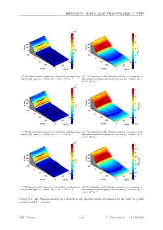
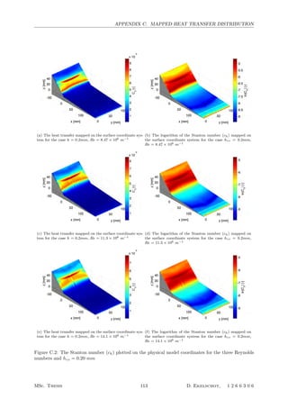
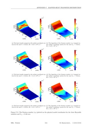
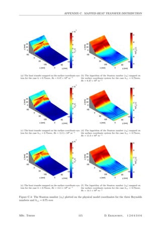
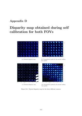
135. APPENDIX E. CONTOUR PLOT OF THE STANDARD DEVIATION IN VX PARALLEL TO THE
5◦
RAMP
−15 −10 −5 0 5 10 15
3
4
5
6
7
y [mm]
z[mm]
Spanwise Vx
distribution at x = 46.97mm
Vx[m/s]
−1000
−995
−990
(a) Vx distribution in the (y,z) plane at x = 47mm
Spanwise velocity std
V
x
at x =46.97
y [mm]
z[mm]
−15 −10 −5 0 5 10 15
3
4
5
6
7
stdV
x
[m/s]
10
15
20
(b) Contour map of stdVx at x = 47mm
−15 −10 −5 0 5 10 15
3
4
5
6
7
y [mm]
z[mm]
Spanwise V
x
distribution at x = 41.06mm
Vx[m/s]
−1000
−995
−990
(c) Vx distribution in the (y,z) plane at x = 41mm
Spanwise velocity std
V
x
at x =41.06
y [mm]
z[mm]
−15 −10 −5 0 5 10 15
3
4
5
6
7
stdV
x
[m/s]
10
15
20
(d) Contour map of stdVx at x = 41mm
−15 −10 −5 0 5 10 15
3
4
5
6
7
y [mm]
z[mm]
Spanwise V
x
distribution at x = 35.16mm
Vx[m/s]−1000
−995
−990
−985
(e) Vx distribution in the (y,z) plane at x = 35mm
Spanwise velocity std
V
x
at x =35.16
y [mm]
z[mm]
−15 −10 −5 0 5 10 15
3
4
5
6
7
stdV
x
[m/s]
10
20
(f) Contour map of stdVx at x = 35mm
−15 −10 −5 0 5 10 15
3
4
5
6
7
y [mm]
z[mm]
Spanwise Vx
distribution at x = 29.25mm
Vx[m/s]
−1000
−995
−990
−985
(g) Vx distribution in the (y,z) plane at x = 29mm
Spanwise velocity stdV
x
at x =29.25
y [mm]
z[mm]
−15 −10 −5 0 5 10 15
3
4
5
6
7
stdV
x
[m/s]
15
20
25
30
(h) Contour map of stdVx at x = 29mm
Figure E.1: Contour map of Vx with its corresponding contour map stdVx
for four different fixed stream-
wise positions on the 5◦
ramp
MSc. Thesis 119 D. Ekelschot, 1 2 6 6 3 0 6

136. Bibliography
J. D. Anderson. Fundamentals of aerodynamics. McGraw-Hill, 2005.
J. D. Anderson. Hypersonic and High-Temperature Gas Dynamics Second Edition. American Institute
of Aeronautics and Astronautics, 2006.
D. Arnal and J. Delery. Laminar-turbulent transition and shock wave/boundary layer interaction. 2004.
C. Atkinson and J. Soria. An efficient simultaneous reconstruction technique for tomographic particle
image velocimetry. Experimental Fluids, 47:553–568, 2009.
P. Bakker and B. van Leer. Gas Dynamics Lecture Notes. TU Delft, 2005.
G. K. Batchelor and J. Miles. Hydrodynamic stability. Cambridge University Press, 1981.
A. Bottaro and P. Luchini. G¨ortler vortices: Are they amenable to local eigenvalue analysis? European
Journal of Mechanics B/Fluids, 1999.
R. Caljouw. An experimental investigation of a three-dimensional hypersonic flow on a double ramp
geometry using stereo-piv. Master’s thesis, TU Delft, 2007.
J. Delery. Shock interference in high mach number flows. La Recherche Aerospatiale, 3:175–185, 1994.
D. Ekelschot. Literature study: Investigation of g¨ortler vortices in hypersonic flow using tomopiv. Tech-
nical report, TU Delft, 2012.
G. Elsinga. Evaluation of aero-optical distortion effects in piv. Experiments in Fluids, 39:246–256, 2005.
G. Elsinga. Tomographic particle image velocimetry and its application to turbulent boundary layers. PhD
thesis, TU Delft, 2008.
G. Elsinga and J. Westerweel. Tomographic-piv measurement of the flow around a zigzag boundary layer
trip. Experimental Fluids, 52:865–876, 2012.
J. Floryan. On the g¨ortler instability of boundary layers. Prog. Aerospace Sci, 28:235–271, 1991.
P. Goulpie, B. G. B. Klingmann, and A. Bottaro. G¨ortler vortices in boundary layers with streamwise
pressure gradient: Linear theory. American Institute of Physics, 1996.
F. Li and M. Malik. Fundamental and subharmonic secondary instabilities of gortler vortices. J. Fluid
Mech., 297:77–100, 1995.
L. Luca de, G. Cardone, D. d. l. C. Aymer, and A. Fonteneau. Goerlter instability of hypersonic boundary
layer. Experiments in Fluids, 16, 1993.
A. Melling. Tracer particles and seeding for particle image velocimetry. Measurement Science and
Technology, 8:1400–1416, 1997.
S. Navarro-Martinez and O. Tutty. Computers and fluids. Numerical simulation of G¨ortler vortices in
hypersonic compression ramps, 34:225–247, 2005.
M. Novara, K. Batenburg, and F. Scarano. Motion tracking-enhanced mart for tomographic piv. Mea-
surement Science and Technology, 21, 2010.
W. Saric. G¨ortler vortices. Annual Review of Fluid Mechanics, 26:379–409, 1994.
120

137. BIBLIOGRAPHY BIBLIOGRAPHY
A. Savitzky and M. Golay. Smooting and differentiation of data by simplfied least squares procedures.
Analytical chemistry, 36(8):1627–1639, 1964.
F. Scarano. Iterative image deformation methods in piv. Measurement Science and Technology, 13, 2002.
F. Scarano. Experimental Aerodynamics. TU Delft, 2007.
F. Schrijer. Experimental investigation of re-entry aerodynamic phenomena. PhD thesis, TU Delft, 2010a.
F. Schrijer. Investigation of g¨ortler vortices in a hypersonic double compression ramp flow by means of
infrared thermography. 10th International Conference on Quatitive InfraRed Thermography, 2010b.
F. Schrijer and W. Bannink. Description and flow assessment of the delft hypersonic ludwieg tube. AIAA,
2008.
F. Schrijer, F. Scarano, and B. van Oudheusden. Application of piv in a mach 7 ludwieg tube flow facility.
6th International Symposium on Particle Image Velocimetry, September 2005.
E. Sch¨ulein and V. Trofimov. Steady longitudinal vortices in supersonic turbulent separated flows. J.
Fluid Mech., pages 1–26, 2011.
D. Schultz and T. Jones. Heat-transfer measurements in short-duration hypersonic facilities. AGARD,
1973.
S. Soloff, R. Adrian, and Z.-C. Liu. Distortion compensation for generalized stereoscopic particle image
velocimetry. Measurement Science and Technology, 8:1441–1454, 1997.
J. Swearingen and R. Blackwelder. The growth and breakdown of streamwise vortices in the presence of
a wall. J. Fluid Mech., 182:255–290, 1987.
B. Wieneke. Volume self-calibration for 3d particle image velocimetry. Exp Fluids, 45:549–556, 2008.
MSc. Thesis 121 D. Ekelschot, 1 2 6 6 3 0 6