This document is the thesis submitted by Bryan Omar Collazo Santiago to the Department of Electrical Engineering and Computer Science at MIT in partial fulfillment of the requirements for a Master of Engineering degree. The thesis presents MLBlocks, a machine learning system that allows data scientists to easily explore different modeling techniques. MLBlocks supports discriminative modeling, generative modeling, and using synthetic features to boost performance. It has a simple interface and is highly parameterizable and extensible. The thesis describes the architecture and implementation of MLBlocks and provides two examples of using it on real-world problems - predicting student dropout in MOOCs and predicting vehicle destinations from trajectory data.


![3.3.5 An Example: Stopout Prediction in MOOCs
An example problem that we translated into this data form is the problem discussed
in Colin Taylor’s thesis of Stopout Prediction in a Massive Open Online Courses[9].
The goal is to predict if and when a student will “stopout” (the online equivalent of
a dropout of a course), given data about his past performance. Here, an Entity is a
Student, the Slices are the different weeks of data, and the Features, are quantities like
average length of forum posts, total amount of time spent with resources, number of
submissions, and many other recorded metrics recorded that talk about the student’s
performance on a given week.
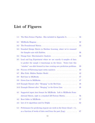
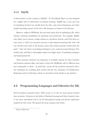
3.3.6 Another Example: Standard 2D Design Matrix
There is one general mapping that already shows that a vast majority of datasets out
there very easily and seamlessly work with MLBlocks. In particular, many datasets,
such as the ones found in the famous UCI Repository and Kaggle competitions, come
in what is also the most common output format of a feature engineering procedure,
which is the 𝑛 x 𝑑 (samples x features) “Design Matrix.” An example is shown in
Figure 3-3 and is commonly denoted as 𝑋 in the literature.
Figure 3-3: Standard Design Matrix in Machine Learning, where we’ve renamed the
Samples axis with Entities.
We claim that this design matrix is simply a special case of the MLBlocks Foun-
dational Matrix, where there is only one slice or one entity in the data. Hence, it can
36](https://image.slidesharecdn.com/b4556345-b79c-4c26-8dc3-6c2a186c38c3-161206014455/85/Machine_Learning_Blocks___Bryan_Thesis-36-320.jpg)
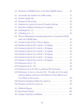
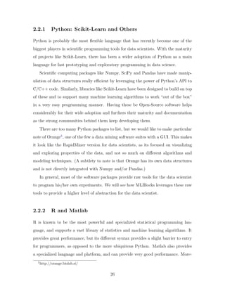
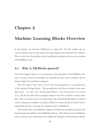
![Figure 3-4: Orange Line: Discriminative Analysis
stock some 𝑗 units of time from now, given data only from the last 𝑖 time units. It
would be nice to experiment with what values of 𝑗 (lead) and 𝑖 (lag) one can use to
predict these problems well.
One way to carry out this type of training and experiment is to “flatten” the data
– which is exactly what the Flatten node in the Orange Line does. We will produce
a 2D Design Matrix from this node which classifiers can use for standard training,
but which will also encode the question of how well we can make predictions given
some lead and lag. In later sections, we’ll also see how to also run such experiments
with Hidden Markov Models (HMMs).
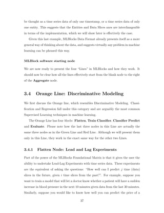
Formally, the transformation in this node goes as follows. Take a timeseries dataset
𝑆 = {𝑠0, 𝑠1, ..., 𝑠 𝑛−1|𝑠𝑡 ∈ R 𝑑
, 𝑡 ∈ [0, 𝑛−1]} with 𝑛 slices in R 𝑑
as shown in Figure 3-5.
Every slice 𝑠𝑡 (also called an observation) has a label and 𝑑 features. Then, given a
lead 𝑗 and a lag 𝑖, we will create a new 2d matrix with data samples 𝐹, where each
new sample 𝑓𝑡 is created by concatenating all the features of the slices in 𝑆 from 𝑡 − 𝑖
to 𝑡 into a single vector, and setting the label of this vector to be the label of the slice
at time 𝑡 + 𝑗.
38](https://image.slidesharecdn.com/b4556345-b79c-4c26-8dc3-6c2a186c38c3-161206014455/85/Machine_Learning_Blocks___Bryan_Thesis-38-320.jpg)


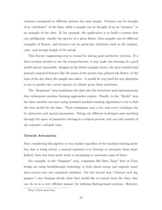
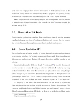
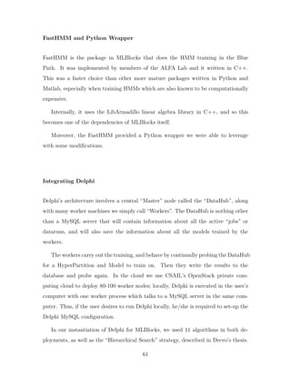
![[MLBlocks]
• line: Orange | Blue | Red | Green. The Line you want to take. :)
• lead: integer. Requires ≥ 0. To be used in all aspects of Lead- Lag experiments.
Nodes that use this are the Flat node, the HMM Predict and the Form HMM
features.
• lag: integer. Requires ≥ 1. To be used in all aspects of Lead- Lag experiments.
Nodes that use this are the Flat node, the HMM Predict and the Form HMM
features.
• test_size: float. Requires 0.0 < 𝑥 < 1.0. Will the percentage of the test set
in the train-test split used in HMM Predict and Train Classifier with Logistic
Regression; Delphi uses a Stratified K-Fold with K=10, and thus will ignore
this.
• num_processes: integer. Positive Integer ≥ 1, number of processes to spawn
in parallelized routines.
• debug: True | False. Controls the level of output in the console.
The next section requests information about the input data. It has five parame-
ters.
[Data]
• data_path: string. Path to folder with CSV files (representing the Founda-
tional Matrix) or path to a single CSV file (representing 2D Matrix).
• data_delimiter: string. Sequence to look for when reading input CSVs. In
most CSVs should be “,” (without quotes).
• skip_rows: integer. Requires ≥ 0. Rows to skip when reading CSVs. Useful
for CSVs with headers.
53](https://image.slidesharecdn.com/b4556345-b79c-4c26-8dc3-6c2a186c38c3-161206014455/85/Machine_Learning_Blocks___Bryan_Thesis-53-320.jpg)
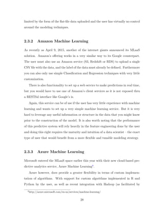
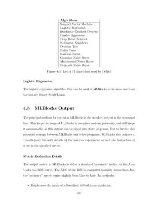
![• label_logic: lambda expression. This is the logic that will be used to get the
label out of every sample. Needs to be a lambda expression as in Python, where
the input is an array-like. Thus, if a label is a column i just have “lambda x:
x[i]”. It supports basic arithmetic operations.
The next sections are now specific to particular nodes and are named accordingly.
[TrainClassifier]
• mode: LogisticRegression | DelphiLocal | DelphiCloud. Discriminative Model-
ing Technique to use.
• learners_budget: integer. Requires ≥ 1. Only used for DelphiCloud; budget
of learners to explore.
• restart_workers: True | False. Only used for DelphiCloud; whether to restart
all the Cloud workers in Delphi. Will yield more throughput, as sometimes there
are straggeler workers in Delphi.
• timeout: integer. Requires ≥ 0. Only used for DelphiCloud; seconds to wait
for DelphiCloud to train. Will come back with results thus far.
[Discretize]
• binning_method: EqualFreq | EqualWidth. Strategy of compute bin cut-
offs. EqualFreq makes the cut-offs be such that every bin has roughly the same
number of instances in the dataset. EqualWidth just divides the range of that
feature in equal length bins.
• num_bins: integer. Requires ≥ 1. Number of bins per feature.
• skip_columns: comma separated integers. e.g. 0,3,8. Indices to skip in
Discretization process. If skipping columns, because say they are already dis-
cretized, you need to make sure they are discretized and 0-indexed.
54](https://image.slidesharecdn.com/b4556345-b79c-4c26-8dc3-6c2a186c38c3-161206014455/85/Machine_Learning_Blocks___Bryan_Thesis-54-320.jpg)
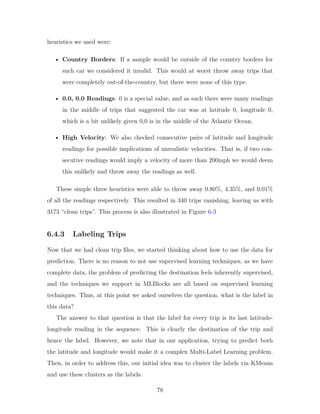
![[HMMTrain]
• mode: Discrete. To be used for switching type of HMM. Only “Discrete” is
supported.
• num_states: integer. Requires ≥ 1. Number of states in the HMM.
• max_iterations: integer. Requires ≥ 1. Sets a maximum number of iterations
for the EM Algorithm.
• log_likelhood_change: float. Requires > 0. Sets the stopping condition for
the EM algorithm.
[Evaluate]
• metric: ACCURACY | ROCAUC | ROCAUCPLOT. Metric to use for evalu-
ation. If ROCAUCPLOT will use matplotlib to plot ROC curve. ROCAUC*
can only be used for binary classification problems.
• positive_class: 0 | 1. Required for ROCAUC* metric; ignored otherwise.
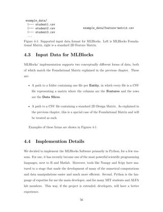
Putting this all together makes the MLBlocks config file. A concrete example can
be found in Appendix B.
MLBConfigManager
To make the parsing of such a file modular, and self-contained, but also to provide
a helper class for developers wanting to use MLBlocks in an automated way, we
constructed an “MLBConfigManager” class that has two main methods; read and
write. The read takes in a path to an INI file and will return a dictionary with all
the key-value pairs already parsed and interpreted. The write takes in any number of
the keyword arguments and an output path, and writes a MLBlocks formated config
file to that path with the specified values, and default values for non-specified.
55](https://image.slidesharecdn.com/b4556345-b79c-4c26-8dc3-6c2a186c38c3-161206014455/85/Machine_Learning_Blocks___Bryan_Thesis-55-320.jpg)


![notion of a ‘Signal’ that maps almost one-to-one with Channel, but lets us discern
readings of a Channel that were used for different Messages.
6.3.1 Trip and Signal Abstraction
Defining good abstractions and concepts is a key part of any system design. In
his influential book The Mythical Man-Month[3], Fred Brooks said that “Conceptual
integrity is the most important consideration in system design”. Thus, we took a
closer look at what important concepts and abstractions we needed to make to be
able to predict destination nicely.
The first one was that of a “Signal,” as introduced in our last section. A Signal is
simply the abstraction of a sequence of (timestamp, value) pairs for a given Channel
and Message pair. This is the main building block of information that we get from
the raw data, and it inherently imposes a times series structure that nicely matches
how the data was generated.
One of the purposes of coming up with such a concept was to flatten the structure
of Channels and Messages to make them easier to think and reason about, and to
help us better discern readings that arose in different messages even though they
used the same channel. With this definition, the raw data reduces to just “a set of
Signals”, which again is much simpler to think about as opposed to its complicated
Message-Channel structure.
The second important concept that we define, and arguably the most important, is
the concept of a Trip. This concept followed immediately from the problem definition
of destination prediction and application. This translates the idea of a ‘sample’ in a
machine learning context to our specific destination prediction problem.
Furthermore, it is imperative that we group them the Signals in terms of the
particular Trip that they were recorded in. This was almost already done for us in
the raw data, as the number of partitions (or .db files) mapped almost one-to-one
with car trips. We say almost because only a subset of the partitions (.db files) were
actually recordings of Signals from where the car started to where it was turned off.
Some other partitions are still valid in light of the other JLR applications, but contain
74](https://image.slidesharecdn.com/b4556345-b79c-4c26-8dc3-6c2a186c38c3-161206014455/85/Machine_Learning_Blocks___Bryan_Thesis-74-320.jpg)


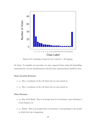
![• 𝑥5: Day of the Month. Ranges from 1 to the number of days of that month in
that year.
• 𝑥6: Hour of the Day. This is the hour when the trip is starting, ranges from
0-23 inclusive.
• 𝑥7: Minutes of the Hour. Ranges from 0-59 inclusive.
Distribution Features
These were 𝐾 + 1 features that represented the conditional distribution on the top-K
locations (and the special not-top-K location), given that the trip has started in this
location. That is, for these features, we looked at all the previous trips that the user
had taken that had started in this same cell. Then, we took the distribution of all
the destinations in those trips. So effectively, every feature 𝑓𝑖 is the proportion of
times you have been to class 𝑖, of all the trips that also started in the current trip’s
location.
• 𝑥𝑖: Conditional Probability of going of going to class 𝑖 given the start location
of this trip. For integers 𝑖 ∈ [1, 𝐾 + 1]
6.5 Results with MLBlocks
The feature matrices created above are a perfect fit for the Orange Line in the ML-
Blocks software. We inputted them and achieved the following results.
6.5.1 Orange Line
Examining the 𝑅 and 𝐾 Parameters
We used two main parameters to phrase the problem of destination prediction. These
were the size 𝑅 of the grid, and the number of locations to predict 𝐾.
We did the variation of 𝑅 on 10, 100 and 1000, and 𝐾 on 10, 20 and ALL (meaning
no-clipping; using all the unique destinations the car has been to). We fixed the car
89](https://image.slidesharecdn.com/b4556345-b79c-4c26-8dc3-6c2a186c38c3-161206014455/85/Machine_Learning_Blocks___Bryan_Thesis-89-320.jpg)


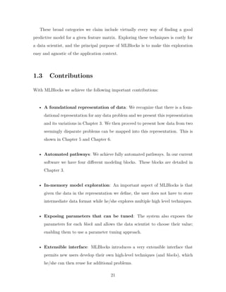
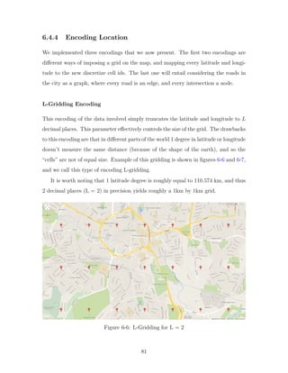
![[MLBlocks]
line=Orange
lead=0
lag=1
test_split=0.3
num_processes=12
debug=False
[Data]
data_path=example_data/
data_delimiter=,
skip_rows=1
label_logic=lambda x: x[0]
[TrainClassifier]
mode=LogisticRegression
learners_budget=5
restart_workers=False
ping_back_seconds=60
[Discretize]
binning_method=EqualFreq
num_bins=5
skip_columns=None
[HMMTrain]
hmm_type=Discrete
num_states=4
max_iterations=10
log_likelihood_change=.0000001
[Evaluate]
evaluation_metric=ACCURACY
positive_class=0
Figure A-3: Example Config File in MLBlocks.
104](https://image.slidesharecdn.com/b4556345-b79c-4c26-8dc3-6c2a186c38c3-161206014455/85/Machine_Learning_Blocks___Bryan_Thesis-104-320.jpg)
![Bibliography
[1] Yu Zheng Xing Xie Jin Huang Andy Yuan Xue, Rui Zhang and Zhenghua Xu.
Destination prediction by sub-trajectory synthesis and privacy protection against
such prediction. In IEEE, 2013.
[2] Anind K. Dey Brian D. Ziebart, Andrew L. Maas and J. Andrew Bagnell. Navigate
like a cabbie: Probabilistic reasoning from observed context-aware behavior. In
ACM, 2008.
[3] Frederick P. Brooks. The Mythical Man-Month: Essays on Software Engineering.
Addison-Wesley, 1995.
[4] Jon Froehlich and John Krumm. Route prediction from trip observations. SAE
International, 2008.
[5] Eibe Frank Ian H. Witten and Mark A. Hall. Data Mining: Practical Machine
Learning Tools and Techniques. 3rd Edition. Morgan Kaufmann Publishers, 2011.
[6] John Krumm. Real time destination prediction based on efficient routes. SAE
International, 2006.
[7] John Krumm and Eric Horvitz. Predestination: Inferring destination from partial
trajectories. In UbiComp, 2006.
[8] Sham Kakade Niranjan Srinivas, Andreas Krause and Matthias Seeger. Gaussian
process optimization in the bandit setting: No regret and experimental design. In
Proceedings of the 27th International Conference on Machine Learning, 2010.
[9] Colin Taylor. Stopout prediction in massive open online courses. Master’s thesis,
Massachusetts Institute of Technology, 2014.
105](https://image.slidesharecdn.com/b4556345-b79c-4c26-8dc3-6c2a186c38c3-161206014455/85/Machine_Learning_Blocks___Bryan_Thesis-105-320.jpg)