This document is a master's thesis submitted by Sascha Nawrot to Berlin University of Applied Sciences in partial fulfillment of the requirements for a Master of Science degree in Applied Computer Science. The thesis introduces novel, lightweight open source annotation tools for whole slide images that enable deep learning experts and pathology experts to cooperate in creating training samples by annotating regions of interest in whole slide images, regardless of platform or format, in a fast and easy manner. The tools consist of a conversion service to convert whole slide images to an open format, an annotation service for annotating regions of interest, and a tessellation service to extract the annotated regions from the images.
![Chapter 1
Introduction
1.1 Motivation
The medical discipline of pathology is in a digital transformation. Instead of
looking at tissue samples through the means of traditional light microscopy, it
is now possible to digitize those samples. This digitalization is done with the
help of a so called slide scanner. The result of such an operation is a whole slide
image (WSI) [11]. The digital nature of WSIs opens the door to the realm of
image processesing and analysis which yields certain benefits, such as the use
of image segmentation and registration methods to support the pathologist in
his/her work.
A very promising approach to image analysis is the use of deep learning, also
known as neural networks (NN). These are a group of computational models
inspired by our current understanding of biological NN. The construct of many
interconnected neurons is considered a NN (both in the biological and artificial
context). Each single one of those neurons has input values and an output
value. Once the input reaches a certain trigger point, the cell in the neuron
sends a signal as output. The connections between the neurons are weighted
and can dampen or strengthen a signal. Because of this, old pathways can be
blocked and new ones created. In other words, a NN is capable of ”learning”
[60]. This is a huge advantage compared to other software models. While
certain problems are ”easier” to solve in a sequential, algorithmic fashion (say
an equation or the towers of hanoi), certain problems (e.g. image segmentation
or object recognition) are very complex, so that new approaches are needed,
while other problems can not be solved algorithmically at all. With the use
of adequate training samples, a NN can learn to solve a problem, much like a
human.
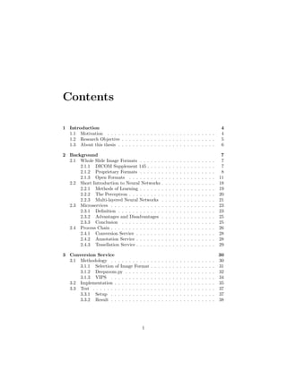
In the recent past the use of NN enabled major breakthroughs, especially in
the area of image classification and object recognition. Karpathy and Fei-Fei,
for example, created a NN that is capable of describing an image or a scene
using natural language text blocks [2] (see fig. 1.1 for a selection of examples).
4](https://image.slidesharecdn.com/5fb6f304-59ac-4e5f-8514-f4f12554de32-161019112150/85/document-7-320.jpg)
![Figure 1.1: Example results of the in [2] introduced model (source: http:
//cs.stanford.edu/people/karpathy/deepimagesent/)
There is enormous potential in the use of NN in the digital pathology as
well, but to transfer these models and technologies, certain obstacles must be
overcome. One of those is the need for proper training samples. While generally
there are large amounts of WSIs (e.g. publicly available at the Cancer Genome
Atlas1
), most of them will not be usable as a training sample without further
preparation.
A possible way to prepare them is by using image annotation: tagging regions
of interest (ROI) on an image and assigning labels or keywords as metadata to
those ROIs. These can be added to the WSIs, stored and later used for training.
The result of such an approach could be similar to the one of Karpathy and Fei-
Fei [2], but with a medical context instead of daily situations.
1.2 Research Objective
The goal of this thesis is the conceptualization and implementation of tools to
enable deep learning and pathology experts to cooperate in annotating WSIs to
create a ground truth for the later use in NNs. In order to do so, it must be
possible to open a given WSI with a viewer, add annotations to it and persist
1https://gdc-portal.nci.nih.gov/
5](https://image.slidesharecdn.com/5fb6f304-59ac-4e5f-8514-f4f12554de32-161019112150/85/document-8-320.jpg)
![those annotations. Additionally, persisted annotations must be extracted from
the WSI to be used as ground truth.
This thesis has three objectives:
(1) There is no standard for WSI files, therefore vendors developed their own
proprietary solutions [11]. This either leads to a vendor lock-in or separate
handling of each proprietary format. To avoid both cases, a conversion tool
that turns proprietary WSI formats into an open format must be introduced.
(2) The deployment of a WSI viewer tool. This WSI viewer must be capable of
adding annotations to a WSI and persisting them. As stated earlier, the tool
is intended to be used by deep learning and pathology experts. An intuitive
and easy-to-understand graphical user interface (GUI) is necessary to avoid
long learning periods and create willingness to actually use the tool.
(3) The implementation of a tool that is capable of turning persisted annota-
tions into a format usable as ground truth.
It is explicitly stated, that the intention of this thesis is to introduce tools
that are used by deep learning and pathology experts to create a ground truth
for NN. The intention is not to create a tool for analyzing and diagnosing WSIs,
that is capable of competing with existing industry solutions.
1.3 About this thesis
This thesis contains 6 chapters.
Chapter 1 - Introduction and 2 - Background address the scope, background
and vocabulary of this thesis.
The chapters 3 to 5 address the components described in the last section:
chapter 3 - Conversion Service will describe a tool for image conversion, chapter
4 - Annotation Service will describe a tool for image annotation and chapter 5 -
Tessellation Service will describe an extraction tool, to prepare the annotations
made with the Annotation Service for the use in a NN.
Finally, Chapter 6 - Conclusion will discuss and conclude the findings of the
aforementioned chapters.
6](https://image.slidesharecdn.com/5fb6f304-59ac-4e5f-8514-f4f12554de32-161019112150/85/document-9-320.jpg)
![Chapter 2
Background
2.1 Whole Slide Image Formats
Due to the amount of data stored in a raw, uncompressed WSI1
, file formatting
and compression are required to make working with WSIs feasible. Since there
is no standardized format for WSIs, vendors came up with their own, propri-
etary solutions, which vary greatly [11]. Efforts of standardization are being
made through the Digital Imaging and Communications in Medicine (DICOM)
Standard [16].
Usually, WSI files are stored as a multitude of single images, spanning mul-
tiple folders and different resolutions. Those files are used to construct a so
called image pyramid [30] (see fig. 2.1 and subsection 2.1.1).
2.1.1 DICOM Supplement 145
Singh et al. [33] describe DICOM as follows:
”Digital Imaging and Communications in Medicine (DICOM),
synonymous with ISO (International Organization for Standardiza-
tion) standard 12052, is the global standard for medical imaging and
is used in all electronic medical record systems that include imaging
as part of the patient record.”
Before Supplement 145: Whole Slide Microscopic Image IOD and SOP
Classes, the DICOM Standard did not address standardization of WSI. Among
others, the College of American Pathologist’s Diagnostic Intelligence and Health
Information Technology Committee is responsible for the creation and further
advancement of this supplement [33].
It addresses every step involved in creating WSIs: image creation, acqui-
sition, processing, analyzing, distribution, visualization and data management
1 A typical 1,600 megapixel slide requires about 4.6 GB of memory on average [30]. The
size of a H&E (hematoxylin and eosin) stained slide ranges typically from 4 to 20 GB [33].
7](https://image.slidesharecdn.com/5fb6f304-59ac-4e5f-8514-f4f12554de32-161019112150/85/document-10-320.jpg)
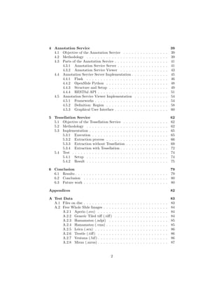
![[16]. It impacted the way how data is stored greatly [33], due to the introduction
of a pyramid image model [16] (see fig. 2.1).
Figure 2.1: DICOMs image pyramid (source: [33])
The image pyramid model facilitates rapid zooming and reduces the com-
putational burden of randomly accessing and traversing a WSI [33], [35]. This
is made possible by storing an image in several precomputed resolutions, with
the highest resolution sitting at the bottom (called the baseline image) and a
thumbnail or low power image at the top (compare fig. 2.1) [16]. This creates a
pyramid like stack of images, hence the name ”pyramid model”. The different
resolutions are referred to as layers [16] or levels [33] respectively.
Each level is tessellated into square or rectangular fragments, called tiles,
and stored in a two dimensional array [30].
Because of this internal organization, the tiles of each level can be retrieved
and put together separately, to either form a subregion of the image or show
it entirely. This makes it easy to randomly access any subregion of the image
without loading large amounts of data [33].
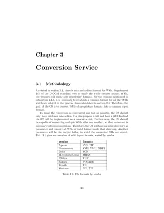
2.1.2 Proprietary Formats
Vendors of whole slide scanners implement their own file formats, libraries and
viewers (see tab. 2.1 for a list of vendors and their formats). Because of this,
they can focus on the key features and abilities of their product. This generally
leads to a higher usability, ease-of-use and enables highly tailored customer
support. Furthermore, in comparison to open source projects, the longevity of
proprietary software is often higher [48].
Since the proprietary formats have little to no documentation, most of the
subsequently presented information was reverse engineered in [21] and [67]. All
proprietary formats listed here implement a modified version of the pyramid
model introduced in 2.1.1
8](https://image.slidesharecdn.com/5fb6f304-59ac-4e5f-8514-f4f12554de32-161019112150/85/document-11-320.jpg)
![vendor formats
Aperio SVS, TIF
Hamamatsu VMS, VMU, NDPI
Leica SCN
3DHistech/Mirax MRXS
Philips TIFF
Sakura SVSLIDE
Trestle TIF
Ventana BIF, TIF
Table 2.1: File formats by vendor
Aperio
The SVS format by Aperio is a TIFF-based format, which comes in a single
file [21]. It has a specific internal organization in which the first image is the
baseline image, which is always tiled (usually with 240x240 pixels). This is
followed by a thumbnail, typically with dimensions of about 1024x768 pixels.
The thumbnail is followed by at least one intermediate pyramid image (compare
fig. 2.1), with the same compression and tile organization as the baseline image
[67]. Optionally, there may be a slide label and macro camera image at the end
of each file [67].
Hamamatsu
Hamamatsu WSIs come in 3 variants:
(1) VMS
(2) VMU
(3) NDPI
(1) and (2) consist of an index file ((1) - [file name].vms, (2) - [file name].vmu)
and 2 or more image files. In the case of (2), there is also an additional op-
timization file. (3) consists of a single TIFF-like file with custom TIFF tags.
While (1) and (3) contain JPEG images, (2) contains a custom, uncompressed
image format called NGR2
[67].
The random access support for decoding parts of jpeg files is poor [67]. To
work around this, so called restart markers are used to create virtual slides.
Restart markers were originally designed for error recovery. They allow a de-
coder to resynchronize at set intervals throughout the image [21]. These markers
are placed at regular intervals. Their offset is specified in a different manner,
depending on the file format. In the case of (1), it can be found in the index
file. In the case of (2), the optimization file holds the information and in the
case of (3), a TIFF tag contains the offset [67].
2For more information on NGR, consult http://openslide.org/formats/hamamatsu/
9](https://image.slidesharecdn.com/5fb6f304-59ac-4e5f-8514-f4f12554de32-161019112150/85/document-12-320.jpg)
![Leica
SCN is a single file format based on BigTIFF that additionally provides a pyra-
midal thumbnail image [21]. The first TIFF directory has a tag called ”Im-
ageDescription” which contains an XML document that defines the internal
structure of the WSI [67].
Leica WSIs are structured as a collection of images, each of which has mul-
tiple pyramid levels. While the collection only has a size, images have a size
and position, all measured in nanometers. Each dimension has a size in pixels,
an optional focal plane number, and a TIFF directory containing the image
data. Fluorescence images have different dimensions (and thus different TIFF
directories) for each channel [67].
Brightfield slides have at least two images: a low-resolution macro image
and one or more main images corresponding to regions of the macro image.
Fluorescence slides can have two macro images: one brightfield and one fluores-
cence [67].
3DHistech/Mirax
MRXS is a multi-file format with complex metadata in a mixture of text and
binary formats. Images are stored as either JPEG, PNG or BMP [21]. The
poor handling of random access is also applicable to PNG. Because of this,
multiple images are needed to encode a single slide image. To avoid having
many individual files, images are packed into a small number of data files. An
index file provides offsets into the data files for each required piece of data. [67].
A 3DHistech/Mirax scanner take images with an overlap. Each picture taken
is then tessellated without an overlap. Therefore, overlap only occurs between
taken pictures [67].
The generation of the image pyramid differs from the process described in
2.1.1 To create the nth
level, each image of the nth
− 1 level is divided by 2 in
each dimension and then concatenated into a new image. Where the nth
− 1
level had 4 images in 2x2 neighborhood, the nth
level will only have 1 image.
This process has no regards for overlaps. Thus, overlaps may occur in the higher
levels of the image pyramid [67].
Philips
Philips’ TIFF is an export from the native iSyntax format. An XML document
with the hierarchical structure of the WSI can be found over the ImageDescrip-
tion tag of the first TIFF directory. It contains key-value pairs based on DICOM
tags [67].
Slides with multiple regions of interest are structured as a single image pyra-
mid enclosing all regions. Slides may omit pixel data for TIFF tiles not in an
ROI. When such tiles are downsampled into a tile that does contain pixel data,
their contents are rendered as white pixels [67].
Label and macro images are stored either as JPEG or as stripped TIFF
directories.
10](https://image.slidesharecdn.com/5fb6f304-59ac-4e5f-8514-f4f12554de32-161019112150/85/document-13-320.jpg)
![Sakura
WSIs in the SVSLIDE format are SQLite 3 database files. Their tables contain
the metadata, associated images and tiles in the JPEG format. The tiles are
addressed as a tupel of focal plane, downsample, level-0 X coordinate, level-0
Y coordinate, color channel . Additionally, each color channel has a separate
grayscale image [67].
Trestle
Trestle’s TIF is a single-file TIFF. The WSI has the standard pyramidic scheme
and tessellation. It contains non-standard metadata and overlaps, which are
specified in additional files. The first image in the TIFF file is the baseline
image. Subsequent images are assumed to be consecutive levels of the image
pyramid with decreasing resolution [67].
Ventana
Ventana’s WSIs are single-file BigTIFF images, organized in the typical pyra-
midical scheme. The images are tiled and have non-standard metadata, as well
as overlaps. They come with a macro and a thumbnail image [67].
2.1.3 Open Formats
As mentioned in 2.1.2, proprietary formats typically come without much or
any documentation. Furthermore, a vendors viewer is usually the only way
of viewing WSIs of a particular format. This creates a vendor lock-in, where
users can not take advantage of new improvements offered by other vendors.
Furthermore, most viewers only provide support for Windows platforms. While,
in a clinical setting, Windows may dominate the market, a significant amount
of users in medical research prefer Linux or Mac OS X [21]. The use of mobile
platforms, such as iOS or Android tablets may also have a great influence of the
work flow in the future. Some vendors try to compensate for this fact with a
server-based approach, which hurts performance by adding a network round-trip
delay on every digital slide operation [21].
To resolve these issues, open image formats have been suggested, which will
be discussed further in the following subsections.
Deep Zoom Images
The DZI format is an XML-based file format, developed and maintained by
Microsoft [64]. A DZI is a pyramidcal, tiled image (see fig. 2.2), similar to the
one described in 2.1.1 (compare 2.1 and 2.2), with two exceptions:
1. the baseline image is referred to as the highest level, instead of the lowest;
this either turns the image pyramid or its labeling upside down
2. tiles are always square, with the exception of the last column/row
11](https://image.slidesharecdn.com/5fb6f304-59ac-4e5f-8514-f4f12554de32-161019112150/85/document-14-320.jpg)
![Figure 2.2: DZI pyramid model example (source: [64])
A DZI consists of two main parts [64]:
(1) a describing XML file ([file name].dzi) with the following metadata:
• format of individual tiles (e.g. JPEG or PNG)
• overlap between tiles
• size of individual tiles
• height and width of baseline image
(2) a directory ([file name] files) containing image tiles of the specified format
(1) and (2) are stored ”next” to each other, so that there are 2 spearate
files. (2) contains sub directories, one for each level of the image pyramid. The
baseline image of a DZI is in the highest level. Each level is tessellated into as
many tiles necessary to go over the whole image, with each tile having the size
specified in the XML file. If the image size is no multiple of the specified tile
size, the width of the nth
column of tiles will be (width mod tile size) pixels.
Equally, the height of the mth
row will be (height mod tile size) pixels. Thus,
the outermost right bottom tile tn,m will be of (width mod tile size) x (height
mod tile size) pixels.
International Image Interoperability Framework
The International Image Interoperability Framework (IIIF) is the result of a
cooperation between The British Library, Stanford University, the Bodleian
Libraries (Oxford University), the Biblioth`eque Nationale de France, Nasjon-
albiblioteket (National Library of Norway), Los Alamos National Laboratory
Research Library and Cornell University [12]. Version 1.0 was published in
2012.
12](https://image.slidesharecdn.com/5fb6f304-59ac-4e5f-8514-f4f12554de32-161019112150/85/document-15-320.jpg)
![IIIFs goal is to collaboratively produce an interoperable technology and com-
munity framework for image delivery [46]. To achieve this, IIIF tries to:
(1) give scholars access to image-based resources around the world
(2) define a set of common APIs to support interoperability between image
repositories
(3) develop and document shared technologies (such as image servers and web
clients), that enable scholars to view, compare, manipulate and annotate
images
Figure 2.3: Example of iiif request (source:http://www.slideshare.
net/Tom-Cramer/iiif-international-image-interoperability-
framework-dlf2012?ref=https://www.diglib.org/forums/2012forum/
transcending-silos-leveraging-linked-data-and-open-image-apis-
for-collaborative-access-to-digital-facsimiles/)
The part relevant for this thesis is (2), especially the image API [27]. It
specifies a web service that returns an image in response to a standard web
request. The URL can specify the region, size, rotation, quality and format of
the requested image (see 2.3). Originally intended for resources in digital image
repositories maintained by cultural heritage organizations, the API can be used
to retrieve static images in response to a properly constructed URL [45]. The
13](https://image.slidesharecdn.com/5fb6f304-59ac-4e5f-8514-f4f12554de32-161019112150/85/document-16-320.jpg)
![URL scheme looks like this 3
:
1 {scheme }://{ s e r v e r }{/ p r e f i x }/{ i d e n t i f i e r }/{ region }/{ s i z e }/{ r o t a t i o n
}/{ q u a l i t y }.{ format }
The region and size parameters are of special interest for this thesis. With
them, it is possible to request only a certain region of an image in a specified
size.
The region parameter defines the rectangular portion of the full image to be
returned. It can be specified by pixel coordinates, percentage or by the value
“full” (see tab. 2.2 and fig. 2.4).
Form Description
full The complete image is returned, without any cropping.
x,y,w,h The region of the full image to be returned is defined in
terms of absolute pixel values. The value of x represents
the number of pixels from the 0 position on the horizontal
axis. The value of y represents the number of pixels from
the 0 position on the vertical axis. Thus the x,y position
0,0 is the upper left-most pixel of the image. w represents
the width of the region and h represents the height of the
region in pixels.
pct:x,y,w,h The region to be returned is specified as a sequence of per-
centages of the full image’s dimensions, as reported in the
Image Information document. Thus, x represents the num-
ber of pixels from the 0 position on the horizontal axis,
calculated as a percentage of the reported width. w repre-
sents the width of the region, also calculated as a percent-
age of the reported width. The same applies to y and h
respectively. These may be floating point numbers.
Table 2.2: Valid values for region parameter (source: [27])
If the request specifies a region whose size extends beyond the actual size
of the image, the response should be a cropped image, instead of an image
with added empty space. If the region is completely outside of the image, the
response should be a ”404 Not Found” HTTP status code [27].
3For detailed information on all parameters see the official API: http://iiif.io/api/
image/2.0
14](https://image.slidesharecdn.com/5fb6f304-59ac-4e5f-8514-f4f12554de32-161019112150/85/document-17-320.jpg)
![Figure 2.4: Results of IIIF request with different values for region parameter
(source: [27])
If a region was extracted, it is scaled to the dimensions specified by the size
parameter (see tab. 2.3 and fig. 2.5).
Figure 2.5: Results of IIIF request with different values for size parameter
(source: [27])
15](https://image.slidesharecdn.com/5fb6f304-59ac-4e5f-8514-f4f12554de32-161019112150/85/document-18-320.jpg)
![If the resulting height or width equals 0, then the server should return a
”400 Bad Request” HTTP status code. Depending on the image server, scaling
above the full size of the extracted region may be supported [27].
Form Description
full The extracted region is not scaled, and is returned at its
full size.
w, The extracted region should be scaled so that its width is
exactly equal to w, and the height will be a calculated value
that maintains the aspect ratio of the extracted region.
,h The extracted region should be scaled so that its height is
exactly equal to h, and the width will be a calculated value
that maintains the aspect ratio of the extracted region.
pct:n The width and height of the returned image is scaled to
n% of the width and height of the extracted region. The
aspect ratio of the returned image is the same as that of
the extracted region.
w,h The width and height of the returned image are exactly
w and h. The aspect ratio of the returned image may be
different than the extracted region, resulting in a distorted
image.
!w,h The image content is scaled for the best fit such that the
resulting width and height are less than or equal to the
requested width and height. The exact scaling may be de-
termined by the service provider, based on characteristics
including image quality and system performance. The di-
mensions of the returned image content are calculated to
maintain the aspect ratio of the extracted region.
Table 2.3: Valid values for size parameter (source: [27])
To use the IIIF API, a compliant web server must be deployed. Loris and
IIPImageserver are examples for open source IIIF API compliant systems [45]:
• Loris, an open source image server based on python that supports the
IIIF API versions 2.0, 1.1 and 1.0. Supported image formats are JPEG,
JPEG2000 and TIFF.
• IIPImage Server, an open source Fast CGI module written in C++, that
is designed to be embedded within a hosting web server such as Apache,
Lighttpd, MyServer or Nginx. Supported image formats are JPEG2000
and TIFF [46].
16](https://image.slidesharecdn.com/5fb6f304-59ac-4e5f-8514-f4f12554de32-161019112150/85/document-19-320.jpg)
![OpenStreetMap/Tiled Map Service
OpenStreetMap (OSM) is a popular tile source used in many online geographic
mapping specifications [45]. It is a community driven alternative to services
such as Google Maps. Information is added by users via aerial images, GPS
devices and field maps. All OSM data is classified as open data, meaning that
it can be used anywhere, as long as the OSM Foundation is credited [41].
Tiled Map Service (TMS) is a tile scheme developed by the Open Source
Geospatial Foundation (OSGF) [45] and specified in [40]. The OSGF is a non-
profit organization whose goal it is to support the needs of the open source
geospatial community. TMS provides access to cartographic maps of geo-referenced
data. Access to these resources is provided via a ”REST” interface, starting
with a root resource describing available layers, then map resources with a set
of scales, then scales holding sets of tiles [40].
Both, OSM and TMS, offer zooming images, which in general, have the
functionality necessary, to be of use for this thesis. Unfortunately, they are also
highly specialized on the needs of the mapping community, with many features
not needed in the context of this thesis.
JPEG 2000
[56] describes the image compression standard JPEG 2000 as follows:
”JPEG 2000 is an image coding system that uses state-of-the-art
compression techniques based on wavelet technology. Its architec-
ture lends itself to a wide range of uses from portable digital cameras
through to advanced pre-press, medical imaging and other key sec-
tors.”
It incorporates a mathematically lossless compression mode, in which the
storage requirement of images can be reduced by an average of 2:1 [15]. Fur-
thermore, a visually lossless compression mode is provided. At visually loss-
less compression rates, even a trained observer can not see the difference be-
tween original and compressed version. The visually lossless compression mode
achieves compression rates of 10:1 and up to 20:1 [50]. JPEG 2000 code streams
offer mechanisms to support random access at varying degrees of granularity. It
is possible to store different parts of the same picture using different quality [15].
In the compression process, JPEG 2000 partitions an image into rectangular
and non-overlapping tiles of equal size (except for tiles at the image borders).
The tile size is arbitrary and can be as large as the original image itself (resulting
in only one tile) or as small as a single pixel. Furthermore, the image gets
decomposed into a multiple resolution representation [62].
This creates a tiled image pyramid, similar to the one described in subsection
2.1.1.
The encoding-decoding process of JPEG 2000 is beyond the scope of this
thesis. Therefore, it is recommended to consult either [50] for a quick overview
or [62] for an in depth guide.
17](https://image.slidesharecdn.com/5fb6f304-59ac-4e5f-8514-f4f12554de32-161019112150/85/document-20-320.jpg)
![TIFF/BigTIFF
The Tagged Image File Format (TIFF) consists of a number of corresponding
key-value pairs (e.g. ImageWidth and ImageLength, who describe the width
and length of the contained image) called tags. One of the core features of this
format is that it allows for the image data to be stored in tiles [20].
Each tile offset is saved in an image header, so that efficient random access
to any tile is granted. The original specification demands a use of 32 bit file
offset values, limiting the maximum offset to 232
. This constraint limits the file
size to be below 4 GB [20].
This constraint led to the development of BigTIFF. The offset values were
raised to a 64 bit base, limiting the maximum offset to 264
. This results in an
image size of up to 18,000 peta bytes [17].
TIFF and BigTIFF are capable of saving images in multiple resolutions.
Together with the feature of saving tiles, the image pyramid model (as described
in subsection 2.1.1) can be applied [18].
2.2 Short Introduction to Neural Networks
The objective of the workflows introduced in chapter 1.2 is to create training
samples for NNs. Before going into other details, it is necessary to clarify what
NNs are, how they work, why they need training samples and what they are
used for4
.
Artificial NNs are a group of models inspired by Biological Neural Networks
(BNN) . BNNs can be described as an interconnected web of neurons (see 2.6),
whose purpose it is to transmit information in the form of electrical signals. A
neuron receives input via dendrites and sends output via axons [71]. An average
human adult brain contains about 1011
neurons. Each of those receives input
from about 104
other neurons. If their combined input is strong enough, the
receiving neuron will send an output signal to other neurons [14].
Figure 2.6: Neuron in a BNN (source: [71])
Although artificial NNs are much simpler in comparison (they seldom have
4 An in-depth introduction into the field of NNs is far beyond the scope of this work.
For further information about NNs, consultation of literature (e.g. [8], [14], [28], [60], [71]) is
highly recommended.
18](https://image.slidesharecdn.com/5fb6f304-59ac-4e5f-8514-f4f12554de32-161019112150/85/document-21-320.jpg)
![more than a few dozen neurons [14]), they generally work in the same fashion.
One of the biggest strengths of a NN, much like a BNN, is the ability to adapt
by learning (as humans, NN learn by training [71]). This adaption is based on
weights that are assigned to the connections between single neurons. Fig 2.7
shows an exemplary NN with neurons and the connections between them.
Figure 2.7: Exemplary NN (source: [71])
Each line in fig. 2.7 represents a connection between 2 neurons. Those con-
nections are a one-directional flow of information, each assigned with a specific
weight. This weight is a simple number that is multiplied with the incoming/out-
going signal and therefore weakens or enhances it. They are the defining factor
of the behavior of a NN. Determining those values is the purpose of training a
NN [14].
According to [71], some of the standard use cases for NN are: pattern recog-
nition, time series prediction, signal processing perceptron, control, soft sensors,
and anomaly detection
2.2.1 Methods of Learning
There are 3 general strategies when it comes to the training of a NN [14]. Those
are:
1. Supervised Learning
2. Unsupervised Learning
3. Reinforcement Learning (a variant of Unsupervised Learning [69])
Supervised Learning is a strategy that involves a training set to which the
correct output is known (a so called ground truth), as well as an observing
teacher. The NN is provided with the training data and computes its output.
This output is compared to the expected output and the difference is measured.
19](https://image.slidesharecdn.com/5fb6f304-59ac-4e5f-8514-f4f12554de32-161019112150/85/document-22-320.jpg)
![According to the error made, the weights of the NN are corrected. The magni-
tude of the correction is determined by the used learning algorithm [69].
Unsupervised Learning is a strategy that is required when the correct output
is unknown and no teacher is available. Because of this, he NN must organize
itself [71]. [69] makes a distinction between 2 different classes of unsupervised
learning:
• reinforced learning
• competitive learning
Reinforced learning adjusts the weights in such a way, that desired output
is reproduced. An example is a robot in a maze: If the robot can drive straight
without any hindrances, it can associate this sensory input with driving straight
(desired outcome). As soon as it approaches a turn, the robot will hit a wall
(non-desired outcome). To prevent it from hitting the wall it must turn, there-
fore the weights of turning must be adjusted to the sensory input of being at a
turn. Another example is Hebbian learning (see [69] for further information).
In competitive learning, the single neurons compete against each other for
the right to give a certain output for an associated input. Only one element in
the NN is allowed to answer, so that other, competing neurons are inhibited [69].
2.2.2 The Perceptron
The perceptron was invented by Rosenblatt at the Cornell Aeronautical Labora-
tory in 1957 [70]. It is the computational model of a single neuron and as such,
the simplest NN possible [71]. A perceptron consists of one or more inputs, a
processor and a single output (see fig. 2.8) [70].
Figure 2.8: Perceptron by Rosenblatt (source: [71])
This can be directly compared to the neuron in fig. 2.6, where:
• input = dendrites
• processor = cell
• output = axon
A perceptron is only capable of solving linearly separable problems, such
as logical AND and OR problems. To solve non-linearly separable problems,
more then one perceptron is required [70]. Simply put, a problem is linearly
20](https://image.slidesharecdn.com/5fb6f304-59ac-4e5f-8514-f4f12554de32-161019112150/85/document-23-320.jpg)
![separable, if it can be solved with a straight line (see fig. 2.9), otherwise it is
considered a non-linearly separable problem (see fig. 2.10).
Figure 2.9: Examples for linearly separable problems (source: [71])
Figure 2.10: Examples for non-linearly separable problems (source: [71])
2.2.3 Multi-layered Neural Networks
To solve more complex problems, multiple perceptrons can be connected to
form a more powerful NN. A single perceptron might not be able to solve XOR,
but one perceptron can solve OR, while the other can solve ¬AND. Those two
perceptrons combined can solve XOR [71].
If multiple perceptrons get combined, they create layers. Those layers can
be separated into 3 distinct types [8]:
• input layer
• hidden layer
• output layer
A typical NN will have an input layer, which is connected to a number of
hidden layers, which either connect to more hidden layers or, eventually, an
output layer (see fig. 2.11 for a NN with one hidden layer).
21](https://image.slidesharecdn.com/5fb6f304-59ac-4e5f-8514-f4f12554de32-161019112150/85/document-24-320.jpg)
![Figure 2.11: NN with multiple layers (source: http://docs.opencv.org/2.4/
_images/mlp.png)
As the name suggests, the input layer gets provided with the raw information
input. Depending on the internal weights and connections inside the hidden
layer, a representation of the input information gets formed. At last, the output
layer generates output, again based on the connections and weights between the
hidden and output layer [8].
Training this kind of NN is much more complicated than training a simple
perceptron, since weights are scattered all over the NN and its layers. A solution
to this problem is called backpropagation [71].
Backpropagation
Training is an optimization process. To optimize something, a metric to mea-
sure has to be established. In the case of backpropagation, this metric is the
accumulated output error of the NN to a given input. There are several ways
to calculate this error, with the mean square error being the most common
one [14]. The mean square error describes the average of the square of the
differences of two variables (in this case the expected and the actual output).
Finding the optimal weights is an iterative process of the following steps:
1. start with training set of data with known output
2. initialize weights in NN
3. for each set of input, feed the NN and compute the output
4. compare calculated with known output
5. adjust weights to reduce error
22](https://image.slidesharecdn.com/5fb6f304-59ac-4e5f-8514-f4f12554de32-161019112150/85/document-25-320.jpg)
![There are 2 possibilities in how to proceed. The first one is to compare
results and adjust weights after each input/output-cycle. The second one is to
calculate the accumulated error over a whole iteration of the input/output-cycle.
Each of those iterations is known as an epoch [14].
2.3 Microservices
The following section elaborates on the concept of Microservices (MS), defining
what they are, listing their advantages and disadvantages, as well as explain-
ing why this approach was chosen over a monolithic approach. A monolithic
software solution is described by [55] as follows:
”[...] a monolithic application [is] built as a single unit. Enter-
prise Applications are often built in three main parts: a client-side
user interface (consisting of HTML pages and javascript running in a
browser on the user’s machine) a database (consisting of many tables
inserted into a common, and usually relational, database manage-
ment system), and a server-side application. The server-side appli-
cation will handle HTTP requests, execute domain logic, retrieve
and update data from the database, and select and populate HTML
views to be sent to the browser. This server-side application is a
monolith - a single logical executable. Any changes to the system
involve building and deploying a new version of the server-side ap-
plication.”
2.3.1 Definition
MS are an interpretation of the Service Oriented Architecture. The concept is to
separate one monolithic software construct into several smaller, modular pieces
of software [79]. As such, MS are a modularization concept. However, they differ
from other such concepts, since MS are independent from each other. This is
a trait, other modularization concepts usually lack [79]. As a result, changes
in one MS do not bring up the necessity of deploying the whole product cycle
again, but just the one service. This can be achieved by turning each MS into
an independent process with its own runtime [55].
This modularization creates an information barrier between different MS.
Therefore, if MS need to share data or communicate with each other, light
weight communication mechanisms must be established, such as a RESTful
API [68].
Even though MS are more a concept than a specific architectural style,
certain traits are usually shared between them [68]. According to [68] and [55],
those are:
(a) Componentization as a Service: bringing chosen components (e.g. ex-
ternal libraries) together to make a customized service
23](https://image.slidesharecdn.com/5fb6f304-59ac-4e5f-8514-f4f12554de32-161019112150/85/document-26-320.jpg)
![(b) Organized Around Business Capabilities: cross-functional teams, in-
cluding the full range of skills required to achieve the MS goal
(c) Products instead of Projects: teams own a product over its full lifetime,
not just for the remainder of a project
(d) Smart Endpoints and Dumb Pipes: each microservice is as decoupled
as possible with its own domain logic
(e) Decentralized Governance: enabling developer choice to build on pre-
ferred languages for each component.
(f) Decentralized Data Management: having each microservice label and
handle data differently
(g) Infrastructure Automation: including automated deployment up the
pipeline
(h) Design for Failure: a consequence of using services as components, is
that applications need to be designed so that they can tolerate the failure
of single or multiple services
Furthermore, [7] defined 5 architectural constraints, which should help to
develop a MS:
(1.) Elastic
The elasticity constraint describes the ability of a MS to scale up or down,
without affecting the rest of the system. This can be realized in different
ways. [7] suggests to architect the system in such a fashion, that multiple
stateless instances of each microservice can run, together with a mechanism
for service naming, registration, and discovery along with routing and load-
balancing of requests.
(2.) Resilient
This constraint is referring to the before mentioned trait (h) - Design for
Failure. The failure of or an error in the execution of a MS must not impact
other services in the system.
(3.) Composable
To avoid confusion, different MS in a system should have the same way of
identifying, representing, and manipulating resources, describing the API
schema and supported API operations.
(4.) Minimal
A MS should only perform one single business function, in which only
semantically closely related components are needed.
(5.) Complete
A MS must offer a complete functionality, with minimal dependencies to
other services. Without this constraint, services would be interconnected
again, making it impossible to upgrade or scale individual services.
24](https://image.slidesharecdn.com/5fb6f304-59ac-4e5f-8514-f4f12554de32-161019112150/85/document-27-320.jpg)
![2.3.2 Advantages and Disadvantages
One big advantage of this modularization is that each service can be written in
a different programming language, using different frameworks and tools. Fur-
thermore, each microservice can bring along its own support services and data
storages. It is imperative for the concept of modularization, that each microser-
vice has its own storage of which it is in charge of [79].
The small and focused nature of MS makes scaling, updates, general changes
and the deployment process easier. Furthermore, smaller teams can work on
smaller code bases, making the distribution of know-how easier [68].
Another advantage is how well MS plays into the hands of agile, scrum and
continuous software development processes, due to their previously discussed
inherent traits.
The modularization of MS does not only yield advantages. Since each MS has
its own, closed off data management (see 2.3.1(f)), interprocess communication
becomes a necessity. This can lead to communicational overhead which has a
negative impact on the overall performance of the system [79].
2.3.1(e) (Decentralized Governance) can lead to compatibility issues, if dif-
ferent developer teams chose to use different technologies. Thus, more com-
munication and social compatibility between teams is required. This can lead
to an unstable system which makes the deployment of extensive workarounds
necessary [68].
It often makes sense to share code inside a system to not replicate function-
ality which is already there and therefore increase the maintenance burden. The
independent nature of MS can make that very difficult, since shared libraries
must be build carefully and with the fact in mind, that different MS may use
different technologies, possibly creating dependency conflicts.
2.3.3 Conclusion
The tools needed to achieve the research objective stated in subsection 1.2 will
be implemented by using the MS modularization patterns. Due to the imple-
mentation being done by a single person, some of the inherent disadvantages of
MS are negated (making them a favorable modularization concept):
• Interprocess communication does not arise between the single stages of the
process chain, since they have a set order (e.g. it would not make sense
trying to extract a training sample without converting or annotating a
WSI first).
• Different technologies may be chosen for the single steps of the process
chain, however, working alone on the project makes technological incom-
patibilities instantly visible
• The services should not share functionality, therefore there should be no
need for shared libraries
25](https://image.slidesharecdn.com/5fb6f304-59ac-4e5f-8514-f4f12554de32-161019112150/85/document-28-320.jpg)
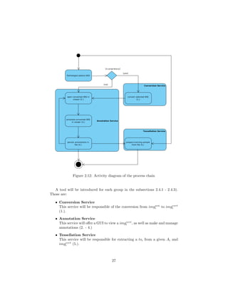
![2.4.1 Conversion Service
The devices which create WSIs, so called whole slide scanners, create images
in various formats, depending on the vendor system (due to the lack of stan-
dardization [11]). The Conversion Service (CS) has the goal of converting those
formats to an open format (compare subsections 2.1.2 and 2.1.3, see fig. 2.13).
Figure 2.13: Visualization of the Conversion Service
Upon invocation, the CS will take every single WSI inside a given directory
and convert it to a chosen open format. The output of each conversion will be
saved in another specified folder. Valid image formats for conversion are: BIF,
MRXS, NDPI, SCN, SVS, SVSLIDE, TIF, TIFF, VMS and VMU.
2.4.2 Annotation Service
As mentioned in 2.4, the Annotation Service (AS) will provide a graphical user
interface to view a WSI, create annotations and manage those annotations. This
also includes persisting made annotations in a file (see fig. 2.14).
Figure 2.14: Visualization of the Annotation Service
The supplied GUI will offer different tools to help the user annotate the
WSI, e.g. a ruler to measure the distance between two points. The annotations
themselves will be made via drawing a contour around an object of interest and
putting a specified label on that region. To ensure uniformity of annotations,
28](https://image.slidesharecdn.com/5fb6f304-59ac-4e5f-8514-f4f12554de32-161019112150/85/document-31-320.jpg)

![3.1.1 Selection of Image Format
A format or service must be chosen as conversion target for the CS. Choices
have been established in 2.1.3. These are: BigTIFF, DZI, IFFF, JPEG 2000
and TMS/OMS.
To convert a WSI, a conversion tool is needed. Tab. 3.2 shows a listing of
possibilities for that purpose. Listed are the name of the tool, the technology
used and the output format. The table indicates, that DZI has a great variety of
options, while the alternatives have little to none (Map Tiler for TMS, Kakadu
for IFFF and none for the others).
tool description output
Deep Zoom Com-
poser
dekstop app for Windows DZI
Image Composite
Editor
dekstop app for Windows DZI
DeepZoomTools.dll .NET library DZI
deepzoom.py python script DZI
deepzoom perl script DZI
PHP Deep Zoom
Tools
PHP script DZI
Deepzoom PHP script DZI
DZT Ruby library DZI
MapTiler desktop app for Windows,
Mac, Linux
TMS
VIPS command line tool, library
for a number of languages
DZI
Sharp Node.js script, uses VIPS DZI
MagickSlicer shell script DZI
Gmap Uploader
Tiler
C++ application DZI
Node.js Deep Zoom
Tools
Node.js script, under con-
struction
DZI
OpenSeaDragon
DZI Online Com-
poser
Web app (and PERL,
PHP scripts)
DZI
Zoomable service, offers embeds; no
explicit API
DZI
ZoomHub service, under construc-
tion
DZI
Kakadu C++ library IIIF
PyramidIO Java tool (command line
and library)
DZI
Table 3.2: Overview of conversion options for zooming image formats (source:
[45])
31](https://image.slidesharecdn.com/5fb6f304-59ac-4e5f-8514-f4f12554de32-161019112150/85/document-34-320.jpg)
![Since the CS should only consist of brief user interaction and be as automated
as possible, desktop and web applications are not valid as tools for conversion.
This excludes Deep Zoom Composer, MapTiler, OpenSeaDragon DZI Online
Composer and Zoomable as possible choices (therefore also excluding (next to
the reasons given in subsection 2.1.3), TMS as possible format).
One of the reasons not to use proprietary formats was the limitation to only
certain operating systems, eliminating Windows-only tools. Those are Image
Composite Editor and DeepZoomTools.dll.
Furthermore, reading the proprietary formats is a highly specialized task,
eliminating most of the leftover choices: deepzoom [5], DZT [19], sharp [42],
MagickSlicer, Node.js Deep Zoom Tools (both use ImageMagick to read im-
ages, which does not support any of the proprietary WSI formats [47]), Gmap
Uploader Tiler [65], Zoomhub [44] and PyramidIO [39].
Kakadu can only encode and decode JPEG 2000 images [45], making it no
valid choice either.
This leaves deepzoom.py and VIPS, both creating DZI as output. Through
the use of OpenSlide, they are both capable of reading all proprietary formats
stated in tab. 3.1 [67].
3.1.2 Deepzoom.py
Deepzoom.py1
is a python script and part of Open Zoom2
. It can either be called
directly over a terminal or imported as a module in another python script. The
conversion procedure itself is analogous for both methods.
If run in a terminal the call looks like the following:
1 $ python deepzoom . py [ options ] [ input f i l e ]
The various options and their default values can be seen in table 3.3. If called
without a designated output destination, deepzoom.py will save the converted
DZI in the same directory as the input file.
option description default
-h show help dialog -
-d output destination -
-s size of the tiles in pixels 254
-f image format of the tiles jpg
-o overlap of the tiles in pixels (0 - 10) 1
-q quality of the output image (0.0 - 1.0) 0.8
-r type of resize filter antialias
Table 3.3: Options for deepzoom.py
1See https://github.com/openzoom/deepzoom.py for further details
2See https://github.com/openzoom for further details
32](https://image.slidesharecdn.com/5fb6f304-59ac-4e5f-8514-f4f12554de32-161019112150/85/document-35-320.jpg)
![The resize filter is applied to interpolate the pixels of the image when chang-
ing its size for the different levels. Supported filters are:
• cubic
• biliniear
• bicubic
• nearest
• antialias
When used as module in another python script, deepzoom.py can simply be
imported via the usual import command. To actually use deepzoom.py, a Deep
Zoom Image Creator needs to be created. This class will manage the conversion
process:
1 # Create Deep Zoom Image Creator
2 c r e a t o r = deepzoom . ImageCreator ( t i l e s i z e =[ s i z e ] ,
3 t i l e o v e r l a p =[ overlap ] , t i l e f o r m a t =[ format ] ,
4 image quality =[ q u a l i t y ] , r e s i z e f i l t e r =[ f i l t e r ] )
The options are analogous with the terminal version (compare tab. 3.3). To
start the conversion process, the following call must be made within the python
script:
1 # Create Deep Zoom image pyramid from source
2 c r e a t o r . create ( [ source ] , [ d e s t i n a t i o n ] )
In the proposed workflow, the ImageCreator opens the input image imgwsi
and accesses the information necessary to create the describing XML file for the
DZI (compare subsection 2.1.3). The needed number of levels is calculated next.
For this, the bigger value of height or width of imgwsi
is chosen (see eq. 3.1)
and then used to determine the number of levels lvlmax
(see eq. 3.2) necessary.
max dim = max(height, width) (3.1)
lvlmax
= log2(max dim) + 1 (3.2)
Once lvlmax
has been determined, a resized version imgdzi
i of imgwsi
will
be created for every level i ∈ [0, lvl − 1]. The quality of imgdzi
i will be reduced
according to the value specified for -q/image quality (see tab. 3.3). The res-
olution of imgdzi
i will be calculated with the scale function (see eq. 3.3) for
both, height and width. Furthermore, the image will be interpolated with the
specified filter (-r/resize filter parameter, see tab. 3.3).
scale = dim ∗ 0.5lvlmax
−i
(3.3)
Once imgdzi
i has been created, it will be tessellated into as many tiles of the
specified size (-s/tile size parameter, see tab. 3.3) and overlap (-o/tile overlap
33](https://image.slidesharecdn.com/5fb6f304-59ac-4e5f-8514-f4f12554de32-161019112150/85/document-36-320.jpg)
![parameter, see tab. 3.3) as possible. If the size of imgwsi
in either dimension
is not a multiple of the tile size, the last row/column of tiles will be smaller by
the amount of (tile size − ([height or width] mod tile size)) pixels.
Every tile will be saved as [column] [row].[format] (depending on the -f/file
format parameter, see tab. 3.3) in a directory named according to the corre-
sponding level i. Each one of those level directories will be contained within
a directory called [filename] files. The describing XML file will be persisted as
[filename].dzi in the same directory as [filename] files.
3.1.3 VIPS
VIPS (VASARI Image Processing System) is described as ”[...] a free image
processing system [...]” [13]. It includes a wide range of different image pro-
cessing tools, such as various filters, histograms, geometric transformations and
color processing algorithms. It also supports various scientific image formats,
especially from the histopathological sector [13]. One of the strongest traits of
VIPS is its speed and little data usage compared to other imaging libraries [52].
VIPS consists of two parts: the actual library (called libvips) and a GUI
(called nip2). libvips offers interfaces for C, C++, python and the command
line. The GUI will not be further discussed, since it is of no interest for the
implementation of the CS.
VIPS speed and little data usage is achieved by the usage of a fully demand-
driven image input/output system. While conventional imaging libraries queue
their operations and go through them sequentially, VIPS awaits a final write
command, before actually manipulating the image. All the queued operations
will then be evaluated and merged into a few single operations, requiring no
additional disc space for intermediates and no unnecessary disc in- and out-
put. Furthermore, if more than one CPU is available, VIPS will automatically
evaluate the operations in parallel [51].
As mentioned before, VIPS has a command line and python interface. In
either case, a function called dzsave will manage the conversion from a WSI to
a DZI. A call in the terminal looks as follows:
1 $ vips dzsave [ input ] [ output ] [ options ]
When called, VIPS will take the image [input], convert it into a DZI and
then save it to [output]. The various options and their default values can be
seen in tab. 3.4.
34](https://image.slidesharecdn.com/5fb6f304-59ac-4e5f-8514-f4f12554de32-161019112150/85/document-37-320.jpg)
![option description default
layout directory layout (allowed: dz, google, zoomify) dz
overlap tile overlap in pixels 1
centre center image in tile false
depth pyramid depth onepixel
angle rotate image during save d0
container pyramid container type fs
properties write a properties file to the output directory false
strip strip all metadata from image false
Table 3.4: Options for VIPS
A call in python has the same parameters and default values. It looks like
this:
1 image = Vips . Image . n e w f r o m f i l e ( input )
2 image . dzsave ( output [ , options ] )
In line 1 the image gets opened and saved into a local variable called im-
age. While being opened, further operations on the image could be done. The
command in line 2 writes the processed image as DZI into the specified output
location.
3.2 Implementation
The first iteration of the CS was a python script using deepzoom.py for the
conversion. This caused severe performance issues. Out of all the image files in
the test set (see section 3.3), only CMU-3.svs (from Aperio, see appendix A.2.1)
could be converted. Other files were either too big, so the process would even-
tually be killed by the operating system, or exited with an IOError concerning
the input file from the PIL imaging library.
The second iteration uses VIPS python implementation, which is capable of
converting all the given test images3
.
The script has to be called inside a terminal in the following fashion:
1 $ python ConversionService . py [ input d i r ] [ output d i r ]
Both the input and the output directory parameter are mandatory, in order
for the script to know where to look for images to convert and where to save
the resulting DZIs.
Upon execution, the main() function will be called, which orchestrates the
whole conversion process. The source code can be seen in the code snippet
below.
3 The CS can be found on the disc at the end of this thesis, see appendix A.1.
35](https://image.slidesharecdn.com/5fb6f304-59ac-4e5f-8514-f4f12554de32-161019112150/85/document-38-320.jpg)
![1 def main () :
2 path = checkParams ()
3 f i l e s = os . l i s t d i r ( path )
4 f o r f i l e in f i l e s :
5 print ( ”−−−−−−−−−−−−−−−−−−−−−−−−−−−−−−−−−−−−−−−−−” )
6 extLen = getFileExt ( f i l e )
7 i f ( extLen != 0) :
8 print ( ” converting ” + f i l e + ” . . . ” )
9 convert ( path , f i l e , extLen )
10 print ( ”done ! ” )
checkParams() checks if the input parameters are valid and, if so, returns
the path to the specified folder or aborts the execution otherwise. Furthermore,
it will create the specified output folder, if it does not exist already. In the
next step, the specified input folder will be checked for its content. getFile-
Ext(file) looks up the extension of each contained file and will either return
the length of the files extension or 0 otherwise. Each valid file will then be
converted with the convert(...) function:
1 # convert image source into . dzi format and copies a l l header
2 # information into [ img ] f i l e s d i r as metadata . txt
3 # param path : d i r e c t o r y of param f i l e
4 # param f i l e : f i l e to be converted
5 # param extLen : length of f i l e extension
6 def convert ( path , f i l e , extLen ) :
7 dzi = OUTPUT + f i l e [ : extLen ] + ” dzi ”
8 im = Vips . Image . n e w f r o m f i l e ( path + f i l e )
9 # get image header and save to metadata f i l e
10 im . dzsave ( dzi , overlap=OVERLAP, t i l e s i z e=TILESIZE)
11 # create f i l e f o r header
12 headerOutput = OUTPUT + f i l e [ : extLen −1] + ” f i l e s /metadata . txt ”
13 bashCommand = ” touch ” + headerOutput
14 c a l l (bashCommand . s p l i t () )
15 # get header information
16 bashCommand = ” vipsheader −a ” + path + f i l e
17 p = subprocess . Popen (bashCommand . s p l i t () , stdout=subprocess . PIPE ,
s t d e r r=subprocess . PIPE)
18 out , e r r = p . communicate ()
19 # write header information to f i l e
20 t e x t f i l e = open ( headerOutput , ”w” )
21 t e x t f i l e . write ( out )
22 t e x t f i l e . c l o s e ()
The name for the new DZI file will be created from the original file name,
however, the former extension will be replaced by ”dzi” (see line 7). OUTPUT
specifies the output directory which the file will be saved to. Next, the image
file will be opened with Vips’ Image class. Afterwards, dzsave(...) will be
called, which handles the actual conversion into the dzi file format. OVERLAP and
TILESIZE are global variables which describe the overlap of the tiles and their
respective size. Their default values are 0 (OVERLAP) and 256 (TILESIZE). The
output will be saved to the current working directory of ConversionService.py,
appending ”/dzi/[OUTPUT]/”.
36](https://image.slidesharecdn.com/5fb6f304-59ac-4e5f-8514-f4f12554de32-161019112150/85/document-39-320.jpg)
![When a WSI gets converted into DZI by the CS, most of the image header
information is lost. To counteract this, a file metadata.txt is created in the
[name] files directory, which serves as container for the header information of
the original WSI (see line 12 and 13).
The console command vipsheader -a is responsible for extracting the header
information (see line 17 - 18). The read information (out in line 18) is then writ-
ten into the metadata.txt file (Line 20 - 22).
3.3 Test
To test the correct functionality of the CS a test data set was needed. OpenSlide
offers a selection of freely distributable WSI files4
, which can be used for that
purpose.
Because of the size of each single WSI file, only 2 are included on the disc
at the end of this thesis (see appendix A.1). The others must be downloaded
separately from the OpenSlide homepage. For a complete listing of the used
test data see appendix A.2.
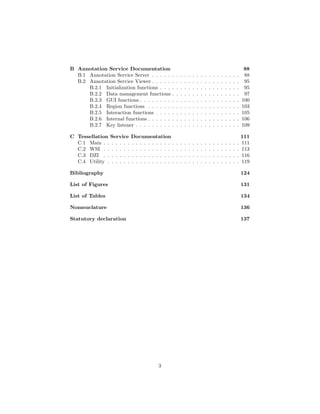
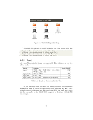
3.3.1 Setup
To create a controlled environment for the test, a new directory will be created,
called CS test. A copy of ConversionService.py as well as a directory containing
all the test WSIs (called input) will be placed in that directory.
Input contains the following slides:
(1) CMU-2 (Aperio, .svs)
(2) CMU-1 (Generic Tiled tiff, .tiff)
(3) OS-3 (Hamamatsu, .ndpi)
(4) CMU-2 (Hamamatsu, .vms)
(5) Leica-2 (Leica, .scn)
(6) Mirax2.2-3 (Mirax, .mrxs)
(7) CMU-2 (Trestle, .tif)
(8) OS-2 (Ventana, .bif)
Because of their structure, (4), (6) and (7) will be placed in directories titled
with their file extension. Fig. 3.1 shows the content of the input folder.
4 See http://openslide.cs.cmu.edu/download/openslide-testdata/ for the test data.
37](https://image.slidesharecdn.com/5fb6f304-59ac-4e5f-8514-f4f12554de32-161019112150/85/document-40-320.jpg)
![Chapter 4
Annotation Service
4.1 Objective of the Annotation Service
As described in 2.4.2, the goal of the AS is to provide a user with the possibility
to:
(1) view a WSI
(2) annotate a WSI
(3) manage previously made annotations
In order to achieve objective (1) - (3), a GUI needs to be deployed which
supports the user in working on those tasks. (3) also adds the need for file
persistence management.
During the development of the AS it became clear that the support of DZI
as the only image format was impractical for the real life environment, thus
making it necessary to support proprietary formats as well. A solution has to
be found, that still addresses the vendor and platform issues stated in 1.2 and
2.1.3.
4.2 Methodology
As stated in 2.1.3, most vendors ship their own implementation of an image
viewer tailored to their proprietary image format, thus creating a vendor lock-
in. Furthermore most of the vendors only support Windows as a platform,
ignoring other operating systems [11], [16], [30]. To avoid vendor- or platform
lock-in, a solution must be found that is independent of operating system and
vendor.
Independence from an operating system can be achieved by using web tech-
nologies, especially when running an application in a web browser, since those
are supported by all modern operating systems and even mobile platforms [23].
39](https://image.slidesharecdn.com/5fb6f304-59ac-4e5f-8514-f4f12554de32-161019112150/85/document-42-320.jpg)
![By choosing the web as target environment for the AS, the service itself
becomes subject to security considerations, namely cross-origin resource sharing
(CORS) [59] and the same-origin policy (SOP) [63]. The SOP is a security
concept of the web application security model, that only allows direct file access
if the parent directory of the originating file is an ancestor directory of the
target file [63]. Since the local WSI file will not have the same origin, CORS
is needed. CORS is a standard that defines mechanisms to allow access to
restricted resources from a domain outside of the origin, when using the HTTP
protocol [59]. Since the WSI is a local file, HTTP can not be used to retrieve
the file.
The restrictions of SOP and CORS can be worked around by deploying a
server as a so called digital slide repository (DSR). A DSR manages storage of
WSIs and their metadata [11]. This way, WSIs would share the same origin as
the viewer and their retrieval would be possible.
Using a DSR has additional advantages:
• WSIs are medical images and as such confidential information. Their
access is usually tied to non-disclosure or confidentiality agreements (e.g.
[66] or [75]). A DSR eliminates the need to hand out copies of WSIs,
which makes it easier to uphold the mentioned agreements.
• WSIs take up big portions of storage [33]. The local systems used by
pathologists in the environment of the AS are usual desktop computers
and laptops. As such, their storage might be insufficient to hold data in
those quantities. A DSR can be set up as a dedicated file server, equipped
for the purpose of offering large amounts of storage.
• A DSR enables centralized file management. Pathologists don’t access
their local version of a WSI and it’s annotations, but share the same data
pool.
• Depending on the network setup, other advantages become possible, e.g.
sharing of rare cases as educational material and teleconsultation of ex-
perts independent of their physical position [22].
Chapter 3 established a service to convert WSIs of various, proprietary for-
mats to DZI, addressing the need to implement multiple image format drivers.
But, as stated in 4.1, a solution to serve proprietary image formats without
explicit conversion is needed as well.
OpenSlides Python provides a DZI wrapper. This wrapper can be used to
wrap a proprietary WSI and treat it as a DZI [67]. A DSR can use this to serve
a proprietary WSI as DZI to a viewer.
For the reasons mentioned above, the AS will be implemented as a web
application. To do so, it will be split into 2 parts: a DSR and a viewer.
40](https://image.slidesharecdn.com/5fb6f304-59ac-4e5f-8514-f4f12554de32-161019112150/85/document-43-320.jpg)
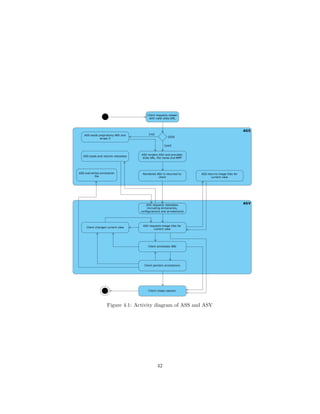
![4.3 Parts of the Annotation Service
As described in section 4.2, the AS will be realized in 2 separate parts:
• a DSR, called Annotation Service Server (ASS) (see subsection 4.3.1)
• a viewer, called Annotation Service Viewer (ASV) (see subsection 4.3.2)
The ASS will be responsible for data management, supplying image data
and serving the ASV to the client. The ASV will provide a WSI viewer with
the tools needed to annotate ROIs in a WSI.
The two components interact as follows: once the client requested a valid
image URL, the ASS will check if the requested WSI is a DZI and, if so, render a
ASV with the image path, the image’s microns per pixel (MPP) and file name.
If the WSI is proprietary, it will be wrapped by OpenSlide. The remaining
procedure is then identical to the DZI case.
The ASV is served to the client as a web application that requests the data
necessary to view the WSI and its annotations. This includes configurations,
previously made annotations (if present), label dictionaries and the image tiles
for the current view. Once loaded, the client can change the current view to
maneuver through the different levels and image tiles available, which will be
requested by the ASS whenever needed. Annotations can be made and persisted
at any time.
Fig. 4.1 visualizes the described interaction process in an activity diagram.
4.3.1 Annotation Service Server
As described in section 4.2, the ASS serves as a DZR. As such it is responsible
for the storage of WSI files and their related metadata [11]. Additional data
managed by the ASS will be:
• annotation data
• the ASV’s configuration data
• dictionary data
Communication with the ASS directly is only necessary to request the ren-
dering of an ASV with a WSI. Once the ASV is rendered, communication can
be handled through shortcuts in the ASV.
41](https://image.slidesharecdn.com/5fb6f304-59ac-4e5f-8514-f4f12554de32-161019112150/85/document-44-320.jpg)
![Communication between ASS and client will be realized over a Represen-
tational State Transfer (REST) API offered by the ASS. REST is an archi-
tectural style for developing web applications. It was established in 2000 by
Fielding in [37]. A system that complies to the constraints of REST can be
called RESTful. Typically, RESTful systems communicate via the HTTP pro-
tocol [37].
The development of a fully functional web server is not within the scope
of this thesis. Therefore, the ASS is intended to run as a local web server.
This works around many of the common issues when hosting a web server (e.g.
inefficient caching, load balance issues, gateway issues, poor security design,
connectivity issues) [3].
4.3.2 Annotation Service Viewer
The ASV is developed to provide a WSI viewer with annotation capabilities. It
serves as the main component for interaction with the AS, realizing most of the
communication with the ASS (compare fig. 4.1).
The annotation capabilities look as follows:
• Annotations will be represented by so called regions. A region is defined
by a path enclosing the ROI. This path can be drawn directly onto the
WSI. The drawing is done either in free hand or polygon mode. When
drawing free hand, the path will follow the mouse cursor along its way as
long as the drawing mode is activated. In polygon mode, segments can
be placed, which are connected with a path in the order that they were
placed in.
• Each region has an associated label that describes the region. A label
is a keyword, predefined by a dictionary. A dictionary contains a list of
keywords that are available as labels.
• New, empty label dictionaries can be created.
• New labels can be added to existing dictionaries.
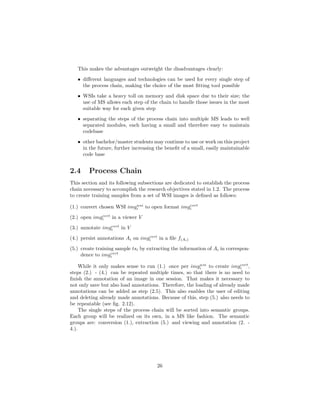
• Each region has a context trait. This trait lists all other regions that
– touch
– cross
– surround
– are surrounded by
the region (see fig. 4.2).
43](https://image.slidesharecdn.com/5fb6f304-59ac-4e5f-8514-f4f12554de32-161019112150/85/document-46-320.jpg)
![• A point of interest (POI) is another way to create a region. After se-
lecting a POI (a point coordinate in the image), an external script will
start a segmentation and return the image coordinates for an enclosing
path to the ASV. The ASV will then automatically create a region based
on the provided information. Since segmentation approaches differ dras-
tically between cases and scenarios [61] (e.g. [25], [26], [36] or [53] for cell
segmentation alone), it exceeds the scope of this work by far. To prove
basic functionality a dummy implementation will be delivered. The script
will be an interchangeable python plug in.
• For annotation support, a distance measurement tool is provided. This
tool can measure the distance between 2 pixels in a straight line. The
measurement will be realized by the euclidean distance between a pixel pa
and pb [74].
Figure 4.2: Example of context regions (B, C are context of A; A, C are context
of B; A, B are context of C; D has no context region)
The ASV uses keywords from a dictionary to label regions. While a free text
approach is more flexible and easier to handle for novice users, it encounters diffi-
culties in a professional metadata environment (such as histopathological image
annotation). A dictionary-based approach facilitates interoperability between
different persons and annotation precision [29]. To increase flexibility, the ASV
will offer the possibility of adding new entries to existing dictionaries.
Since the vocabulary may vary strongly between different studies, the ASV
offers the possibility to create new dictionaries. This way, dictionaries can be
filled with a few case-relevant keywords instead of many generic, mostly irrele-
vant ones. This explicitly does not exclude the use of a generic dictionary if it
should serve a broad series of cases.
44](https://image.slidesharecdn.com/5fb6f304-59ac-4e5f-8514-f4f12554de32-161019112150/85/document-47-320.jpg)
![The first iteration of the ASV will be based on an open source project called
MicroDraw1
(see fig. 4.3 for MicroDraw’s GUI).
Figure 4.3: Microdraw GUI with opened WSI
MicroDraw is a web application to view and annotate ”high resolution his-
tology data” [4]. The visualization is based on OpenSeadragon (OSD)2
, another
open source project. Annotations are made possible by the use of Paper.js3
.
This delivers a baseline for the capabilities stated earlier in this section.
Each iteration of the ASV will be reviewed regarding its usability and func-
tionality by a pathologist, thus adjusting it to its real life environment with each
iteration.
4.4 Annotation Service Server Implementation
The ASS is a local server, implemented in python (as server.py). It offers
a RESTful styled API for communication (see subsection 4.4.4). To improve
functionality, the following frameworks were used:
• Flask (see subsection 4.4.1)
• OpenSlide Python (see subsection 4.4.2)
All code snippets in the following subsections have been taken from as
server.py. A detailed documentation of the individual functions can be found
in appendix B.1.
1See https://github.com/r03ert0/microdraw for more information on the MicroDraw
project
2 See https://openseadragon.github.io/ for more information on OSD.
3 See http://paperjs.org/ for more information on Paper.js.
45](https://image.slidesharecdn.com/5fb6f304-59ac-4e5f-8514-f4f12554de32-161019112150/85/document-48-320.jpg)
![4.4.1 Flask
To give ASS its server capabilities, Flask was used4
. It provides a built-in
development server, integrated unit testing, RESTful request dispatching and is
Web Server Gateway Interface (WSGI) compliant [38]. The WSGI is a standard
interface for the communication between web servers and web applications or
frameworks in python. The interface has a server and application side. The
server side invokes a callable object that is provided by the application side.
The specifics of providing this object are up to the individual server [6].
Flask’s so called route() decorator provides a simple way to build a RESTful
API for server client communication:
1 @app . route ( ’ / loadJson ’ )
2 def loadJson () :
3 . . .
4
5 @app . route ( ’ / createDictionary ’ )
6 def createDictionary () :
7 . . .
8
9 @app . route ( ’ / g e t D i c t i o n a r i e s ’ )
10 def g e t D i c t i o n a r i e s () :
11 . . .
12
13 @app . route ( ”/ runSegmentation ” )
14 def runSegmentation () :
15 . . .
Decorating a function with @app.route([URL]) will bind it to the supplied
URL. When the client requests that bound URL, the server will call the dec-
orated function [38]. The code snippet above shows exemplary how to use
decorators.
A bound URL can also contain variable sections, which are marked as <vari-
able name>. Optionally, a converter can by used to only accept variables of a
certain type. This becomes possible by specifying the converter in front of the
variable: <converter:variable name> [38]. The following code snippet shows
possible examples for URLs with variables (see tab. 4.1 for a list of available
converters):
1 @app . route ( ’ / wsi/<path : f i l e p a t h >. dzi ’ )
2 def index dzi ( f i l e p a t h ) :
3 . . .
4
5 @app . route ( ’ / wsi/<path : f i l e p a t h >’ )
6 def index wsi ( f i l e p a t h ) :
7 . . .
8
9 @app . route ( ’/<slug >. dzi ’ )
10 def dzi ( slug ) :
11 . . .
4 See http://flask.pocoo.org/ for additional information on Flask.
46](https://image.slidesharecdn.com/5fb6f304-59ac-4e5f-8514-f4f12554de32-161019112150/85/document-49-320.jpg)
![To bind a URL with one or more variables, the corresponding function must
be parameterized with the same variables (compare line 1 and 2 or 13 - 14 and
15) [38].
name accepted input
string any text without a slash (default)
int integer values
float floating point values
path like string, but also accepts slashes
any matches one of the items provided
uuid UUID strings
Table 4.1: Available converters in Flask (source: [38])
HTTP provides different methods for accessing URLs (such as GET or
POST) [73]]. By default Flask will answer only GET requests. Any other
method is answered with a ”405 Method not allowed” HTTP status code [38].
This can be changed by adding the methods argument to the decorator:
1 @app . route ( ’ / saveJson ’ , methods=[ ’POST ’ ] )
2 def saveJson () :
3 . . .
Tab. 4.2 states a number of URLs, that have been bound to a corresponding
function. For a detailed documentation of the individual functions, consult
appendix B.1.
URL function
/wsi/<path:file path>.dzi index dzi(file path)
/wsi/<path:file path> index wsi(file path)
/<slug>.dzi dzi(slug)
/<slug> files/<int:level> <int:col>
<int:row>.<format>
tile(slug, level,
col, row, format)
/saveJson saveJson()
/loadJson loadJson()
/createDictionary createDictionary()
/static/dictionaries/<dictionary> loadDictionary(
dictionary)
/getDictionaries getDictionaries()
/switchDictionary switchDictionary()
/runSementation runSegmentation()
Table 4.2: ASS’ URL-function binding overview
47](https://image.slidesharecdn.com/5fb6f304-59ac-4e5f-8514-f4f12554de32-161019112150/85/document-50-320.jpg)
![4.4.2 OpenSlide Python
To read a WSI, ASS uses OpenSlide Python, which is a python interface to the
OpenSlide C library. Besides providing an interface to read a WSI, it offers a
DZI wrapper [67], called DeepZoomGenerator (DZG). The DZG can be used to
create Deep Zoom tiles on demand. The following formats are supported by
OpenSlide [67]: BIF, NDPI, MRXS, SCN, SVS, SVSLIDE, TIF, TIFF, VMS
and VMU. This list is identical to the list of image formats supported by the
CS (compare chapter 3). This is due to the fact that VIPS uses OpenSlide to
read a WSI as well [13].
OpenSlide can read a proprietary WSI as a so called OpenSlide object (see
line 4):
1 from openslide import o p e n s l i d e
2 from openslide . deepzoom import DeepZoomGenerator
3
4 s l i d e = o p e n s l i d e ( s l i d e path )
5 dzg = DeepZoomGenerator ( s l i d e [ , t i l e s i z e , overlap , limit bounds ] )
An OpenSlide object offers methods to access available metadata, image
tiles, the thumbnail image and associated images, if available. The OpenSlide
object can be wrapped with a DZG to enable DZI support (see line 5) [67]. A
number of optional parameters can be passed into the constructor as well (see
tab 4.3 for parameters and their default values).
parameter type description (default value)
osr OpenSlide,
ImageSlide
the slide object (mandatory)
tile size integer the width and height of a single tile
(254)
overlap integer the number of extra pixels to add to
each interior edge of a tile (1)
limit bounds boolean true to render only the non-empty
slide region (false)
Table 4.3: DZG parameters (source: [67])
The DZG5
generates all data necessary, to work with a proprietary WSI as
if it would be a DZI [67]. The DZG’s get dzi(format) and get tile(level,
address) functions are of special importance. get dzi(format) generates a
string containing the complete metadata of a DZI XML file (compare subsection
2.1.3 - Deep Zoom Images). The parameter format specifies the format (PNG or
JPEG) of the individual Deep Zoom tiles. get tile(level, address) returns
an image of the tile corresponding to the provided parameter values (see tab.
4.4). The tiles are returned either as PNG or JPEG, depending on which format
was chosen for get dzi(format).
5 For an in-depth list of functions, see http://openslide.org/api/python/
48](https://image.slidesharecdn.com/5fb6f304-59ac-4e5f-8514-f4f12554de32-161019112150/85/document-51-320.jpg)
![name type description
level integer the DZI level to get the tile from
address tuple the address of the tile within the level as a
(column, row) tuple
Table 4.4: Description of get tile(level, address) parameters (source: [67])
The use of the DZG enables ASS to create DZI metadata and Deep Zoom
tiles from proprietary WSI files on demand.
4.4.3 Structure and Setup
Flask requires a specific directory structure to access static files and HTML
templates. Static files are served from a static/ directory, render-able view
templates must be stored in a template directory. Both of those directories must
be at the root level of the ASS [38]. Because of this, the following directory and
file structure was chosen:
• AnnotationService/
– static/
∗ css/
∗ cursors/
∗ dictionaries/
∗ img/
∗ lib/
∗ segmentation/
∗ wsi/
∗ configuration.json
∗ slideDictionaries.json
– templates/
∗ as viewer.html
– as server.py
As mentioned before, static/ contains all static files required by the ASS,
e.g. the CSS files (css/), icons (cursors/, img/) and JavaScript files (lib/)
needed by the ASV.
To make a WSI accessible to the AS, it must be placed in wsi/. From there,
the file path is arbitrary. wsi/ contains also the persisted annotations of the
associated WSIs. A WSI file will have a save file for each dictionary, according
to the following naming pattern: [file name].[extension] [dictionary].json.
49](https://image.slidesharecdn.com/5fb6f304-59ac-4e5f-8514-f4f12554de32-161019112150/85/document-52-320.jpg)
![parameter description default
-B, –ignore-bounds render only the non-empty slide region false
-e, –overlap set overlap between adjacent tiles in pixels 0
-f, –format set tile format (PNG or JPEG) JPEG
-l, –listen set IP address to listen to 127.0.0.1
-p, –port set port to listen to 5000
-Q, –quality set JPEG compression quality in % 100
-s, –size set tile size 256
Table 4.6: Parameters for as server.py
To retrieve a WSI from the ASS, the URL must be pointed to it in the fol-
lowing manner: http://[host]:[port]/wsi/[file path] (see fig. 4.4 for an example).
Figure 4.4: Example URL to retrieve WSI (http://127.0.0.1:5000/wsi/CMU-
1.svs) ; WSI source: OpenSlides freely distributable test data (see appendix
A.2.1)
4.4.4 RESTful API
The ASS provides a RESTful API. This was realized with Flasks route() dec-
orators (compare subsection 4.4.1). Tab. 4.2 shows a list of corresponding
functions. The listing below gives an overview of the URLs provided by the
API:
(1) - /wsi/[file path].dzi
method: GET
Requests an ASV to view the requested DZI. [file path] must point to a
valid DZI, otherwise a ”404 Not Found” HTTP status code is returned.
Returns either a rendered ASV, which requests the DZI at [file path] or
”404 Not Found”
51](https://image.slidesharecdn.com/5fb6f304-59ac-4e5f-8514-f4f12554de32-161019112150/85/document-54-320.jpg)
![(2) - /wsi/[file path]
method: GET
Works similar to (1), except that the requested image is a proprietary WSI
instead of a DZI. Thus, a DZG is created to wrap the slide.
Returns a specifically generated URL ([slug].dzi).
(3) - /[slug].dzi
method: GET
Requests the DZI metadata of [slug] from the DZG. A corresponding DZG
will only exist, if (2) was called beforehand. Never call this function man-
ually, to ensure a safe execution of the related commands. The ASV will
call this function automatically.
Returns the DZI metadata generated by the DZG or ”404 Not Found” if
no corresponding DZG was found.
(4) - /[slug] files/[level] [col] [row].[format]
method: GET
Requests the Deep Zoom tile [col] [row].[format] in [level] from the DZG.
As with (3), do not call this function manually. The ASV will call it
automatically to retrieve the image tiles needed.
Returns the image tile in the specified level at the requested position or
”404 Not Found” if no image tile could be generated.
(5) - /saveJson
method: POST
Post request that saves the provided JSON data in the provided JSON
file. Creates a new one, if it does not exist. The posted data must look
like the following:
1 {
2 ” f i l e ” : ” [ f i l e name ] ” ,
3 ” content ” : ” [ json content ]”
4 }
5
(6) - /loadJson?src=[source]
method: GET
Loads the JSON file specified in [source].
Returns the JSON data if a file was found, an empty JSON map (”[]”)
otherwise.
(7) - /static/dictionaries/[dictionary]
method: GET
Loads the dictionary file located at [dictionary].
Returns a stringified version of the dictionary content if a dictionary was
found at [dictionary], a ”404 Not Found” HTTP status code otherwise.
52](https://image.slidesharecdn.com/5fb6f304-59ac-4e5f-8514-f4f12554de32-161019112150/85/document-55-320.jpg)
![(8) - /createDictionary?name=[name]&slide=[slide]
method: GET
Requests the creation of a new, empty dictionary. The file will be called
[name]. The ASV adds a ”.json” if necessary. A manual call of this
functions makes an added ”.json” necessary. Otherwise, a text file will be
created. The slide parameter provides the name of the WSI the dictionary
was created at, so it can be changed in the slideDictionaries.json file.
Returns the name and path to the new dictionary as json:
1 {
2 ”name ” : ” [ name ] ” ,
3 ”path ” : ” [ d i c t i o n a r y path ]”
4 }
5
or ”error” if [name] is already taken by another dictionary.
(9) - /getDictionaries
method: GET
Requests a list of files contained in the dictionaries folder.
Returns a list with the file names, or ”-1” if no dictionaries are present.
(10) - /switchDictionary?name=[name]&slide=[slide]
method: GET
Changes the key-value entry in the slideDictionaries.json file whose key
matches the provided [slide] parameter. The value will be adjusted to
[name].
Returns a ”200 OK” HTTP status code.
(11) - /runSegmentation?x=[x]&y=[y]
method: GET
Requests the invocation of the segmentation script provided in the con-
figuration file. The coordinates of the POI are passed as URL arguments
and will be handed down to the segmentation script.
Returns a list of 2D coordinates, describing the contour around the POI,
or a ”404 Not Found” HTTP status code if no script was provided or the
provided script was not found.
53](https://image.slidesharecdn.com/5fb6f304-59ac-4e5f-8514-f4f12554de32-161019112150/85/document-56-320.jpg)
![4.5 Annotation Service Viewer Implementation
The ASV is a browser application based on the MicroDraw open source project.
It provides a client with a WSI viewer with annotation capabilities (see subsec-
tion 4.3.2). It is implemented using JavaScript, HTML5 and CSS. The following
frameworks were used to add additional functionality:
• jQuery
• OSD
• Paper.js
The ASV consists of the following files:
• as viewer.html (template/)
• as viewer.js (static/lib/)
• as viewer.css (static/css/)
• style.css (static/css/)
A documentation of the individual functions of the ASV JavaScript (as server.js)
can be found in appendix B.2.
4.5.1 Frameworks
The ASV uses jQuery, OSD and Paper.js for additional functionality.
jQuery is a common JavaScript library, that offers an API to handle HTML
document traversal and manipulation, event handling, animation and Asyn-
chronous JavaScript and XML (AJAX) requests [58]. AJAX is a group of tech-
nologies which enable a client to make asynchronous web requests [9]. jQuery
is also supported by all common web browsers [57]. The ASV uses jQuery espe-
cially for its HTML document traversal and manipulation capabilities, as well
as its AJAX support.
See the corresponding subsections for OSD and Paper.js.
OpenSeadragon
OSD is used by the ASV to show a WSI. It is a JavaScript based, open source
web application to serve a viewer for ”high-resolution zoomable images” [45]. It
supports the following image formats: DZI, IIIF, OSM and TMS.
Furthermore, custom tile sources can be added to support other image for-
mats as well. Since the ASS is capable of delivering every WSI as DZI, no
custom tile source implementation is necessary for proprietary WSIs.
54](https://image.slidesharecdn.com/5fb6f304-59ac-4e5f-8514-f4f12554de32-161019112150/85/document-57-320.jpg)
![The ASV defines a placeholder block element in its HTML file, which will
be used to hold the OSD viewer (OSDV):
1 <!−− OpenSeadragon viewer −−>
2 <div id=” openseadragon1 ” s t y l e=”width : vh ; height : hh”></ div>
as viewer.html
The OSDV is then created in the ASV’s JavaScript file:
1 // create image viewer
2 viewer = OpenSeadragon ({
3 id : " openseadragon1 " ,
4 p r e f i x U r l : staticPath + "/lib/ openseadragon /images/" ,
5 showReferenceStrip : false ,
6 showNavigator : true ,
7 sequenceMode : false ,
8 navigatorId : "myNavigator " ,
9 zoomPerClick : 1 ,
10 }) ;
as viewer.js
The relation between the <div> element in the webpage and OSDV is cre-
ated through the id parameter (line 3). A description of the other used param-
eters of the OpenSeadragon constructor is provided in Tab. 4.7 6
.
parameter description
id Id of the element to append the viewer’s
container element to.
prefixUrl Prepends the provided prefixUrl to the
path for the OSDVs internal images.
showReferenceStrip If true, display a scrolling strip of image
thumbnails for navigating through the im-
ages.
showNavigator Makes the navigator minimap visible if
true.
sequenceMode Set to true to view a sequence of images.
navigatorId The ID of a div to hold the navigator min-
imap.
zoomPerClick The distance to zoom in on every mouse
click. Setting it to 1.0 disables the feature.
Table 4.7: Overview of used options in OSDV constructor (source: [45])
The OSDV provides a function called zoomPerClick that enhances the im-
age section under the cursor when clicked. Since drawing paths and managing
6 See https://openseadragon.github.io/docs/OpenSeadragon.html#.Options for an in-
depth documentation of every parameter available.
55](https://image.slidesharecdn.com/5fb6f304-59ac-4e5f-8514-f4f12554de32-161019112150/85/document-58-320.jpg)
![regions involves clicking onto the corresponding ROIs, this function must be
disabled. If not disabled, each interaction with an ROI or region will lead to a
call of zoomPerClick, which creates a highly disorienting experience.
Since DZI implements a version of the tiled image pyramid model (compare
subsection 2.1.1), a number of image tiles must be opened to display a current
view. For this purpose the OSDV provides an open(tileSources) function.
The tileSources are provided as URL to the DZI’s metadata file by the ASS
(either ”/static/wsi/[file].dzi” (natural DZI) or ”/static/slide.dzi” (artificial DZI
from the DZG (compare subsection 4.4.2). Based on the URL extension (always
”.dzi” in this AS’ scope), the OSDV selects an appropriate TileSource interface
to access the individual tiles and levels of the provided image format.
A scalebar is added to the OSDV to support the assessment of ROIs:
1 var mpp = 0;
2 i f ( s l i d e .mpp) {
3 ppm = s l i d e .mpp > 0 ? (1 e6 / s l i d e .mpp) : 0
4 }
5
6 viewer . s c a l e b a r ({
7 type : OpenSeadragon . ScalebarType .MICROSCOPE,
8 minWidth : ’150 px’ ,
9 pixelsPerMeter :ppm,
10 c o l o r : ’black ’ ,
11 fontColor : ’black ’ ,
12 backgroundColor : "rgba (255 ,255 ,255 ,0.5)" ,
13 barThickness : 4 ,
14 l o c a t i o n : OpenSeadragon . ScalebarLocation .TOP RIGHT,
15 xOffset : 5 ,
16 yOffset :5
17 }) ;
as viewer.js
The scale is pixels/µm. Since the ASS only delivers MPP (which is µm/pixel)
and the OSDV’s scalebar expects pixels/m (PPM ), a conversion is necessary:
PPM =
106
MPP
(4.1)
Eq. 4.1 can be seen in line 3 of the code snippet above. If no valid input
is provided from the ASS (that is: when no value was specified for MPP in the
WSI’s metadata), PPM will be set to 0. If the pixelPerMeter parameter of
the scalebar equals 0 it is automatically hidden [45]. The options in line 7 - 16
concern the styling of the scalebar (such as color, position and size).
When navigating through the tiles and layers of the OSDV’s tile source, it
will automatically load the tiles needed for the current view from the ASS via
HTTP GET requests [45].
56](https://image.slidesharecdn.com/5fb6f304-59ac-4e5f-8514-f4f12554de32-161019112150/85/document-59-320.jpg)
![Paper.js
The ASV utilizes Paper.js to create a region’s path. Paper.js is an ”open source
vector graphics scripting framework”, running on top of the HTML5 canvas [54].
It offers an API to create and manage vector graphics and bezier curves7
. Ad-
ditionally, it offers vector relevant entities, such as point, size and rectangle
objects and enables the drawing of finely grained paths.
When the OSDV opens an image, a so called annotation overlay (AO) is
created:
1 viewer . addHandler ( ’open ’ , function () {
2 initAnnotationOverlay () ;
3 [ . . . ]
4 }
Excerpt from initAnnotationService() in as viewer.js
The AO is a canvas which is placed above the OSDV. On it, paths can be
drawn, which will be used to enclose an ROI. The AO is initialized in initAnno-
tationOverlay() (see line 2 in the code snippet above). Once created, the AO
is resized to fit the opened WSI in height and width. This only happens when
initializing the canvas. Therefore the AO will have (and keep) the dimensions
of the level the WSI was opened in.
This leads to issues when zooming in and out on the OSDV (and conse-
quently changing the level of the tile source). To counteract this, the AO is
stretched to fit the new dimensions of the WSI’s currently viewed layer. This
leads to the problem of having different pixel densities in AO and OSDV.
The supported granularity of the AO is very fine and, when added program-
matically, can create path segments within the decimals of a single pixel [54]. In
drawing mode however, segments are only added between whole pixels, making
it impossible to draw regions in high zoom levels. Since both, AO and OSDV,
calculate clicked pixel positions from the clicked pixel in the browser [45,54], a
conversion is possible. Two conversion functions haven been implemented:
(1) AO coordinate → image coordinate
(2) image coordinate → AO coordinate
The corresponding functions are convertPathToImgCoordinates(point)
for (1) and convertImgToPathCoordinates(point) for (2). The following code
snippet shows their implementation:
7 A bezier curve is a parametric curve, frequently used in computer graphics [74].
57](https://image.slidesharecdn.com/5fb6f304-59ac-4e5f-8514-f4f12554de32-161019112150/85/document-60-320.jpg)
![1 function convertPathToImgCoordinates ( point ) {
2 // convert to screen coordinates
3 var screenCoords = paper . view . projectToView ( point ) ;
4 // convert to viewport coordinates
5 var viewportCoords = viewer . viewport . pointFromPixel (new
OpenSeadragon . Point ( screenCoords . x , screenCoords . y) ) ;
6 // convert to image coordinates
7 var imgCoords = viewer . viewport . viewportToImageCoordinates (
viewportCoords ) ;
8 return imgCoords ;
9 }
10
11 function convertImgToPathCoordinates ( point ) {
12 // convert to viewport coordinates
13 var viewportCoords = viewer . viewport . imageToViewportCoordinates (
point ) ;
14 // convert to screen coordinates
15 var p i x e l = viewer . viewport . pixelFromPoint ( viewportCoords ) ;
16 // convert to project coordinates
17 var projectCoords = paper . view . viewToProject ( p i x e l ) ;
18 return projectCoords ;
19 }
as viewer.js
convertPathToImgCoordinates(point) receives a point that is in the AO
coordinate system and turns it into a screen coordinate (line 3). The screen
coordinate is converted into a viewport coordinate (line 5) from where it can
be turned into an actual image coordinate (line 7). A viewport coordinate
maps coordinates into values within the interval [0, 100] for both dimensions x
and y, instead of using pixel coordinates [45].
convertImgToPathCoordinates(point) receives a point coordinate of
the baseline image, which is turned into a viewport coordinate (line 13).
The viewport coordinate is turned into a screen coordinate (line 15), to
be turned into an AO coordinate from there (line 17).
Both of those functions need to work with the viewport coordinates to create
a relation between the dimensions of the image and the current level.
4.5.2 Definition: Region
The basic concept used to realize annotations in the ASV are regions. Each
region has a context, imgCoords, name, path, uid and zoom property as
shown in tab. 4.8. They contain the connecting information between an ROI
(imgCoords, path) and its label (name), making them the interface between
visual and textual information. Because of their central importance to the
ASV, this section describes the region object and its properties.
58](https://image.slidesharecdn.com/5fb6f304-59ac-4e5f-8514-f4f12554de32-161019112150/85/document-61-320.jpg)
![:Region
context : Array
imgCoords : OpenSeadragon.Point[1..n]
name: String
path: Paper.Point[1..n]
uid: Integer
zoom: Float
Table 4.8: Class diagram of the region class
The context property is a list of unique label ids of other regions (compare
subsection 4.3.2). If there is a region R1 and a region R2, then the label of R2
is added to the context of R1, if:
• R2’s path touches, crosses, surrounds or is surrounded by R1’s path, and
• R2’s label is not in the context list of R1 already, and
• R2’s label = R1’s label
The imgCoords (image coordinates) property represents the coordinates of
the path’s segments in the baseline image. They are represented as a list of
1 to n Openseadragon.Points8
. This property is used to establish the relation
between the ROIs of the AO and the baseline image.
The name property contains the title of the region’s corresponding label. A
region is created with the dictionary label entry currently active at the time of
the regions creation.
The path property represents the coordinates of the path’s segments in the
AO. It is a list of 1 to n Paper.Points9
. They are being used to manage the
contour of an ROI in the AO. The number of points in imgCoords and path is
always identical, as is their position inside the list.
The uid is a unique id (uid ∈ Z+
) that is used to identify the region.
The zoom attribute describes the level of magnification at the point a region
was created. It is the ratio between displayed and original image size (e.g.
1 = 1:1 ratio, 0.5 = 1:2 ratio). This information is added due to the fact
that the annotation process seldom happens in the highest nor at a singular
magnification. Instead, different magnifications are used (lower ones to speed
up the process, higher ones to inspect ROIs in more detail). This leads to
annotations that are rarely pixel precise and tend to contain numerous false
positives and negatives [1].
8 See https://openseadragon.github.io/docs/OpenSeadragon.Viewport.html#
viewportToImageCoordinates for more information on OSD’s Point class.
9 See http://paperjs.org/reference/point/ for more information on Paper.js’ Point
class.
59](https://image.slidesharecdn.com/5fb6f304-59ac-4e5f-8514-f4f12554de32-161019112150/85/document-62-320.jpg)
![4.5.3 Graphical User Interface
This subsections describes the GUI of the ASV and its individual elements
(compare fig. 4.5 for reference):
[1] Toolbar
The toolbar menu contains the Help button ([2]), toolbar toggle switch ([3]),
navigation map ([4]), dictionary list ([5]) and the label list ([6]).
[2] Help button
Hovering over the help button shows a tooltip containing the hotkey mapping
of the ASV.
[3] Toolbar toggle
The toolbar toggle switch can be used to show and hide the toolbar.
[4] Navigation map
The navigation map shows a macro image of the currently opened WSI and
highlights the viewed area.
[5] Dictionary list
The dictionary list shows the currently selected dictionary. A left click on
it opens a list with all currently available dictionaries from which a new one
can be selected. Once selected the old labels will be removed and the new
labels loaded instead.
[6] Label list
The label list lists all available annotation labels from the loaded dictionary.
The selected label is highlighted (see Gef¨aß (vessel) in fig. 4.5). Other labels
can be selected by a mouse click. Additionally, the labels can be iterated via
the tab key. A click on the eye symbol on top of the list toggles the visibility
of all regions. A click on the eye symbol to the left of the label name toggles
the visibility of all regions associated with that label. The color of a label
can be changed with a click on the colored square. This will also change the
color of all regions which are already drawn and associated to that label.
[7] OSDV and AO
The OSDV with its AO and exemplary regions.
[8] Example of a region
Example of a ”sonstige” (miscellaneous) labeled region.
60](https://image.slidesharecdn.com/5fb6f304-59ac-4e5f-8514-f4f12554de32-161019112150/85/document-63-320.jpg)
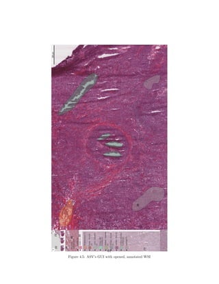
![Chapter 5
Tessellation Service
5.1 Objective of the Tessellation Service
The objective of the TS is to provide a service that extracts image regions
annotated by the AS to create samples for the training of a NN. In this context,
”extraction” describes the process of creating sub images of the original image,
which contain all of the annotated ROI and as little of anything else as possible.
Additionally, the correspondence with the associated region label must be kept.
The AS uses regions to describe ROIs (compare subsection 4.5.2). Those regions
are persisted in a JSON file. Therefore, the TS has 2 objectives:
(1) parse a JSON file and acquire its region data
(2) extract ROIs based on the acquired region data
The handling of WSIs is complicated due to their size and file formats. To
avoid unnecessary complication, the TS will use common file types (JPEG, PNG
and TXT) for the extraction.
5.2 Methodology
The objective of the TS is to create usable training samples for NNs, as stated in
section 5.1. Depending on the setup, chosen learning method (compare section
2.2) and purpose of the NN, the requirements imposed on the training samples
may vary. Smith demonstrates in [72] exemplary how to train a NN to recognize
letters in images of written text by training it with 10x10 pixel grayscale images
(256 gray levels/pixel) of letters. Shereena and David introduce a novel content
based image retrieval classification method in [77], based on color and texture
features. Other approaches extract features through the use of mathematical
models from the supplied images (such as edges or shapes) [32].
62](https://image.slidesharecdn.com/5fb6f304-59ac-4e5f-8514-f4f12554de32-161019112150/85/document-65-320.jpg)
![Because of those varying requirements, the TS will be capable of producing
different output:
(1) Unaltered image of ROI
(2) Resize images to a specific width and height
(3) Approximate ROIs via tessellation
(4) Convert extracted images to grayscale
A user can draw a region’s path without any restrictions concerning the
pattern, resulting in ROIs that can be of arbitrary shape. Therefore, bounding
boxes (BB) are used for ROI extraction in the cases (1) and (2) (see fig. 5.1
for an example). A BB is a rectangular body, fully enclosing a provided (two
dimensional) object of arbitrary shape [76].
Figure 5.1: Examplary BBs: B1 is BB of M1, B2 is BB of
M2 (source: http://www.idav.ucdavis.edu/education/GraphicsNotes/
Bounding-Box/Bounding-Box.html)
In the case of (1), an ROI’s BB is copied pixel by pixel into a new image.
The resizing (scaling the output image up or down to the provided pixel values)
in the case of (2) makes preprocessing of the BB necessary. This has 2 reasons:
• If the aspect ration of the provided width and height is different than the
one of the BB, the resulting image will be distorted.
• When scaling images down, interpolation can be used, to reduce the in-
formation loss of the image [31]. This is partially possible when scaling
images up as well, e.g. via fractal interpolation, but a non trivial task [24].
Therefore, the size of the BB will be adjusted to match the aspect ratio of
the provided width and height. If the resulting BB is bigger then the provided
width and height, the image will be scaled down and interpolated. If the BB
is smaller, it will be scaled up instead of the image. This leads to a bigger
63](https://image.slidesharecdn.com/5fb6f304-59ac-4e5f-8514-f4f12554de32-161019112150/85/document-66-320.jpg)
![area inside the BB that is not part of the ROI, but a pixel ratio of 1:1 between
original and extracted image, resulting in no distortion or loss of quality.
Case (3) approximates a ROI by tessellating it into tiles of the provided
width and height. Tessellation describes the tiling of a plane using one or more
geometric shapes with no overlaps or gaps (see fig. 5.2 for an example) [10].
Every tile inside the region’s enclosing path (or touched by it) is targeted by
the extraction. Each tile is extracted into an individual image.
Figure 5.2: Example of an ROI approximated via tessellation (gray tiles belong
to the ROI)
Cases (1) - (3) can be combined with (4) to convert the extracted ROI images
into grayscale images.
A region contains additional information besides the label that can be uti-
lized, especially the level of magnification (compare subsection 4.5.2). As Doyle
has shown in [34], the level of magnification an annotation was made in is an
important factor. This is due to the fact that manual annotations made in lower
magnifications do not have the granularity needed for higher ones, which results
in numerous false positives and negatives and therefore distorts the ground
truth [1]. A region’s zoom attribute informs at what level of magnification a
region was drawn in, thus helping to assess the described issue.
To utilize the additional metadata, each extracted region will also have a
corresponding metadata file. This metadata contains:
• the name of the extracted image file (case (1) and (2)), or a list of all
image tiles which belong to the ROI (case (3))
• the region’s label
• the level of magnification
• the region’s context
64](https://image.slidesharecdn.com/5fb6f304-59ac-4e5f-8514-f4f12554de32-161019112150/85/document-67-320.jpg)
![Section 5.1 additionally stated the objective of keeping up correspondence
between an ROI and its associated label. To achieve this, an extracted image
will be saved in a directory of the same name as its corresponding label. This
way, all ROIs of a specific label can be collected in one location. Additionally,
the corresponding metadata file will contain an association between image file
and label name.
5.3 Implementation
The TS is implemented as a python script called TessellationService.py1
.
As stated in sections 5.1 and 5.2, its purpose is to extract annotated ROIs from
a WSI. This is done with the help of the following frameworks and libraries:
OpenSlide, NumPy, Pillow and OpenCV (Open Source Computer Vision Li-
brary).
OpenSlide was used to access and read a provided WSI (compare subsection
4.5.1 - OpenSlide).
NumPy is a python library for efficient scientific computing, especially re-
garding operations involving multi-dimensional array objects [78]. Since a lot
of image operations are based on the use of matrices, this library was used to
increase efficiency.
OpenCV is an open source computer vision and machine learning library. It
was built to provide a common infrastructure for computer vision applications.
It offers numerous functions regarding image processing and machine learning
[43]. Its main purpose in the TS is to create a reference image for the tessellation
function (see subsection 5.3.4).
Pillow is an imaging library, which offers methods to read from and write to
image files. It was used for reading, writing, scaling and converting the extracted
images.
A detailed documentation of the TS’ functions can be found in appendix C.
5.3.1 Execution
The TS can be called over the python interpreter:
1 $ python T e s s e l l a t i o n S e r v i c e [ input ] [ d i c t i o n a r y ] [ params ]
The [input] and [dictionary] arguments are mandatory.
Files whose ROIs are supposed to be extracted are passed to the TS via the
[input] argument. This can be a list of WSIs, DZIs and directories. If a directory
is handed to the TS, all subdirectories (except a DZI’s ” files” directory) will
be searched as well.
As mentioned in subsection 4.4.3, each used dictionary has its own save file
per WSI annotated with it, according the the pattern [file name].[extension]
[dictionary].json. The [dictionary] parameter is used to determine which save
1 The TS is contained on the disc at the end of this thesis, see appendix A.1.
65](https://image.slidesharecdn.com/5fb6f304-59ac-4e5f-8514-f4f12554de32-161019112150/85/document-68-320.jpg)
![file to use. The provided directory name is applied to all input elements. Each
file must have its associated save file in the same directory.
As mentioned in section 5.2, it might be necessary to create different output
images for different purposes. Therefore, the TS has a list of optional parameters
to manipulate the created output in order to be applicable to a wider variety of
cases (see tab. 5.1). Those parameters are optional.
name description default
-h, –help show help -
-f, –force-overwrite flag to overwrite images with the
same name (if not supplied, a
number will be added to the im-
age name)
false
-g, –grayscale flag to convert images to
grayscale images before saving
them
false
-i, –interpolation choose interpolation method:
nearest neighbor, bilinear,
bicubic, lanczos
nearest neighbor in-
terpolation
-o, –output [direc-
tory]
choose output directory (if not
provided, the TS will save all
extracted images in its current
working directory)
-
-r, –resize [width]
[height]
resize all output images to the
provided [width] and [height] in
pixel
-
-s, –show-
tessellated
flag to create window and show
stitched image resulting from the
tessellation process (only for de-
bugging purposes, see ”-t”)
false
-t, –tessellate
[width] [height]
tessellate regions into tiles of the
provided [width] and [height] in
pixels
-
Table 5.1: Optional parameters for the TS
5.3.2 Extraction process
The TS receives a list of files and folders to extract regions from and iterates
over each entry. If the entry is a directory, each contained element will be
checked for its type. If it is a WSI/DZI file, the extraction is started right away.
Once the extraction is finished, the next element is examined. If the entry is a
directory, each contained element is subject to the same evaluation. WSI/DZI
files are extracted, while subdirectories are recursively traversed until the end of
66](https://image.slidesharecdn.com/5fb6f304-59ac-4e5f-8514-f4f12554de32-161019112150/85/document-69-320.jpg)
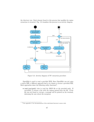
![• save image(image, region, slide name, *tiles) generates an appro-
priate name from the region information and the slide name for the im-
age and metadata file. The name differs between tessellated and non-
tessellated output (see tab. 5.3).
If -r is provided, the image will be resized to the supplied height and width,
with the interpolation method provided via -i (default: nearest neighbor
interpolation). If -g is specified, the image will be converted to grayscale
with the luma transform defined in the ITU-R 601-2 standard [49] (see eq.
5.1).
L = R ∗ 299/1000 + G ∗ 587/1000 + B ∗ 114/1000 (5.1)
Eq. 5.1 averages out the RGB values of every pixel under consideration
of how a human eye perceives colors.
If -o was provided, the processed image will be saved in the supplied
location inside a directory with the name of the extracted region’s label.
• save metadata(name, region, *tiles) writes the corresponding meta-
data to an extracted image into a file (see tab. 5.3 for the file name
pattern). The metadata is a JSON map and contains the values listed in
tab. 5.2. When the TS is run with -t, the ”image” key is replaced by
”tiles”, which is a JSON list containing the names of all tile image files
belonging to the extracted image (each file name is in accordance with the
pattern in tab. 5.3).
key value type
context the image region’s context JSON list
image name of the extracted image file (com-
pare tab. 5.3)
string
tiles list of file names of the extracted tiles
(compare tab. 5.3)
JSON list
label the region’s label string
zoom the region’s zoom float
Table 5.2: Metadata information
• get bounding box(region) iterates over every segment of a region’s path
and builds the BB by collecting the minimal and maximal values for x and
y (compare fig. 5.1).
• resize bounding box(bounding box) is used to adjust a region’s BB to
a different aspect ratio. This is to avoid image distortion when the -r
parameter specifies a different image ratio than the BB’s inherent one
(see fig. 5.4 for an example).
68](https://image.slidesharecdn.com/5fb6f304-59ac-4e5f-8514-f4f12554de32-161019112150/85/document-71-320.jpg)
![Figure 5.4: Example for adjusted BB (A - original BB with aspect ratio of ∼1:1,
B - adjusted BB to aspect ratio of ∼1:2)
• scale bounding box(bounding box, scale) scales a BB by a provided
scale. This is to avoid image distortions due to scaling images up (compare
section 5.2). While get bounding box(region) changes the aspect ratio
of a BB, scale bounding box(bounding box, scale) keeps the aspect
ratio and increases or decreases both dimensions of the BB by the provided
scale.
name image file metadata file
-t not provided [slide name] [region.uid].
jpeg
[slide name] [region.uid].
metadata.json
-t provided [slide name] [region.uid]
([row] [column]).jpeg
[slide name] [region.uid].
metadata.tessellated.json
Table 5.3: File name patterns of generated output
5.3.3 Extraction without Tessellation
As mentioned in subsection 5.3.2, the implementation of the extraction process
differs for DZI and WSI. This is because of the use of OpenSlide to read a WSI.
The following two subsections describe the extraction process for both cases. A
documentation of all mentioned functions can be found in appendix C.
69](https://image.slidesharecdn.com/5fb6f304-59ac-4e5f-8514-f4f12554de32-161019112150/85/document-72-320.jpg)
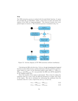
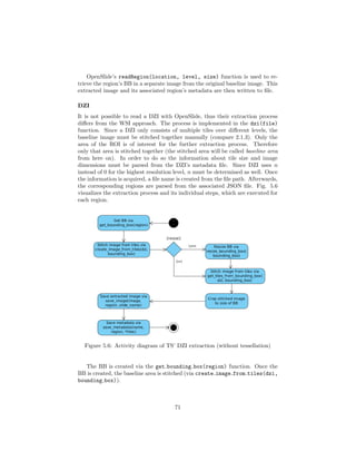
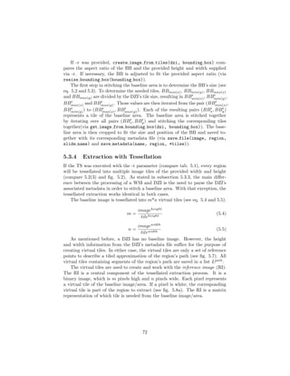
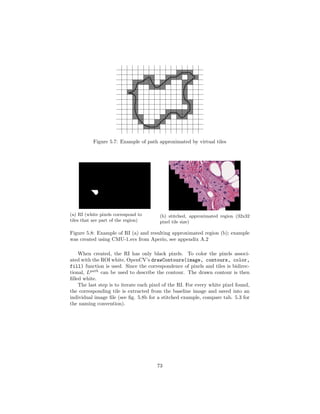
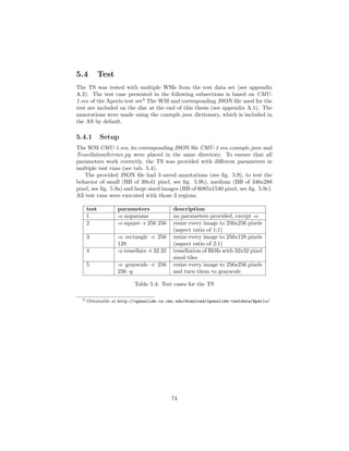
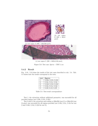
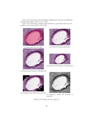
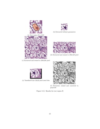
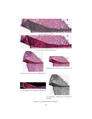
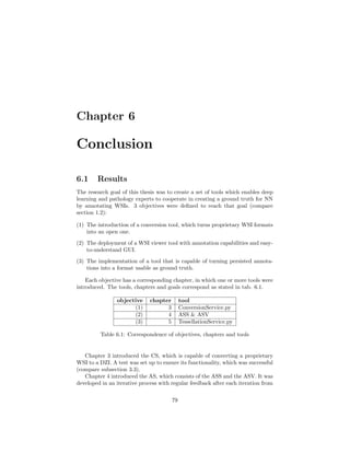
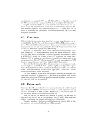

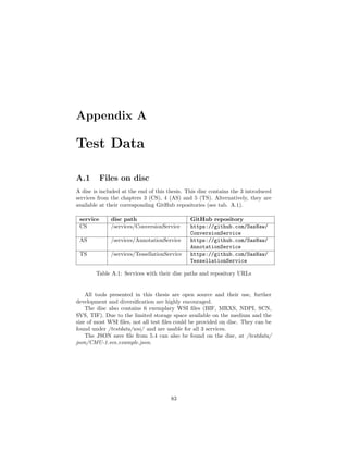
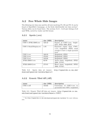
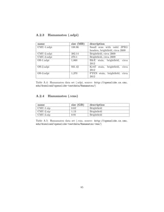
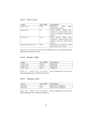
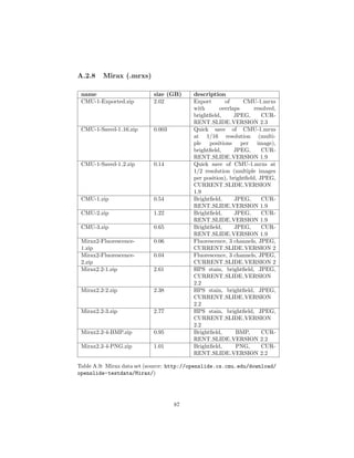
![Appendix B
Annotation Service
Documentation
The following two sections document the implemented functions of the ASS
(section B.1) and ASV (section B.2) in detail.
B.1 Annotation Service Server
getDictionary() is a utility function that fetches the dictionary associated
with the current WSI/DZI from the slideDictionaries.json file1
.
It first opens slideDictionaries.json, creates a python dictionary from its
content and tries to fetch the value corresponding to the WSI/DZI’s name (line
2 - 4). If a value was found, it is returned (line 5 - 6), otherwise a new entry is
created. The key is the WSI/DZI’s file name, the value is the default dictionary
from the configuration.json file, which is then returned (line 7 - 11).
getDictionary()
1 def getDictionary ( f i l e p a t h ) :
2 with open (SLIDE DICTIONARIES , ’ r ’ ) as f i l e :
3 dictioary map = json . loads ( f i l e . read () )
4 d i c t i o n a r y = dictioary map . get ( f i l e p a t h )
5 i f d i c t i o n a r y :
6 return d i c t i o n a r y
7 e l s e :
8 dictioary map [ f i l e p a t h ] = DEFAULT DICTIONARY
9 with open (SLIDE DICTIONARIES , ’w ’ ) as f i l e :
10 f i l e . write ( json . dumps( dictioary map ) )
11 return DEFAULT DICTIONARY
1 Compare subsection 4.4.3
88](https://image.slidesharecdn.com/5fb6f304-59ac-4e5f-8514-f4f12554de32-161019112150/85/document-91-320.jpg)
![index dzi()
If the client requests a DZI (URL ends in ”.dzi”), index dzi() renders an
ASV and passes the necessary information (slide URL, file name, MPP and
dictionary) to it.
It builds the file name and slide URL (line 3 and 4) for a requested DZI.
A metadata.txt will be present in the [slide name] files directory, if the DZI
was created with the CS. If so, the function will try to fetch the metadata
information about MPP and calculate the average size of a pixel (line 6 - 16). If
the MPP metadata could not be fetched, it is set to 0 (line 17 - 18). File name,
URL, MPP and dictionary are passed to the ASV, which is rendered with the
given information (line 19).
1 @app . route ( ’ / wsi/<path : f i l e p a t h >. dzi ’ )
2 def index dzi ( f i l e p a t h ) :
3 file name = f i l e p a t h + ’ . dzi ’
4 s l i d e u r l = ’ / wsi / ’ + file name
5 # read dzi f i l e
6 try :
7 with open ( ’ s t a t i c / wsi / ’ + f i l e p a t h + ’ f i l e s /metadata . txt ’ ) as
f i l e :
8 mpp x = 0
9 mpp y = 0
10 metadata = f i l e . read () . s p l i t ( ’ n ’ )
11 f o r property in metadata :
12 i f openslide .PROPERTY NAME MPP X in property :
13 mpp x = property . s p l i t ( ’ : ’ ) [ 1 ]
14 e l i f openslide .PROPERTY NAME MPP Y in property :
15 mpp y = property . s p l i t ( ’ : ’ ) [ 1 ]
16 slide mpp = ( f l o a t (mpp x) + f l o a t (mpp y) ) / 2
17 except IOError :
18 slide mpp = 0
19 return render template ( ’ as viewer . html ’ , s l i d e u r l=s l i d e u r l ,
slide mpp=slide mpp , file name=file name , d i c t i o n a r y=
getDictionary ( file name ) )
index wsi()
When the client requests a proprietary WSI (URL does not end in ”.dzi”),
index wsi() renders an ASV and passes the necessary information (slide URL,
file name, MPP and dictionary) to it. Furthermore, it wraps a DZG around the
proprietary WSI and adds that to the WSGI object.
Line 1 - 8 create a map with the optional DZG parameters (compare tab.
4.3) and turn them into a dictionary. Line 9 reads the proprietary WSI. A DZG
with the supplied parameters2
is created, which wraps the proprietary slide
object to add Deep Zoom support (line 9 - 12). The created DZG is added to
the WSGI object (line 10). Line 13 - 18 fetch associated images, the metadata
(line 14), wrap the associated images with a DZG of their own and add this,
together with the metadata, to the WSGI object. Line 19 - 24 fetch the MPP
2Compare tab. 4.6
89](https://image.slidesharecdn.com/5fb6f304-59ac-4e5f-8514-f4f12554de32-161019112150/85/document-92-320.jpg)
![metadata and calculate the average MPP (or set it to 0, if not found). Line 25
creates a URL for the DZG object with Flasks url for(endpoint, **values)
function. This URL is passed, together with the MPP, file path and dictionary,
to an ASV which then gets rendered (line 26).
1 @app . route ( ’ / wsi/<path : f i l e p a t h >’ )
2 def index wsi ( f i l e p a t h ) :
3 config map = {
4 ’DEEPZOOM TILE SIZE ’ : ’ t i l e s i z e ’ ,
5 ’DEEPZOOM OVERLAP’ : ’ overlap ’ ,
6 ’DEEPZOOM LIMIT BOUNDS ’ : ’ limit bounds ’ ,
7 }
8 opts = d i c t (( v , app . c o n f i g [ k ] ) f o r k , v in config map . items () )
9 s l i d e = o p e n s l i d e ( ’ s t a t i c / wsi / ’ + f i l e p a t h )
10 app . s l i d e s = {
11 SLIDE NAME: DeepZoomGenerator ( s l i d e , ∗∗ opts )
12 }
13 app . associated images = [ ]
14 app . s l i d e p r o p e r t i e s = s l i d e . p r o p e r t i e s
15 f o r name , image in s l i d e . associated images . items () :
16 app . associated images . append (name)
17 slug = s l u g i f y (name)
18 app . s l i d e s [ slug ] = DeepZoomGenerator ( ImageSlide ( image ) , ∗∗ opts )
19 try :
20 mpp x = s l i d e . p r o p e r t i e s [ openslide .PROPERTY NAME MPP X]
21 mpp y = s l i d e . p r o p e r t i e s [ openslide .PROPERTY NAME MPP Y]
22 slide mpp = ( f l o a t (mpp x) + f l o a t (mpp y) ) / 2
23 except ( KeyError , ValueError ) :
24 slide mpp = 0
25 s l i d e u r l = u r l f o r ( ’ dzi ’ , slug=SLIDE NAME)
26 return render template ( ’ as viewer . html ’ , s l i d e u r l=s l i d e u r l ,
slide mpp=slide mpp , file name=f i l e p a t h , d i c t i o n a r y=
getDictionary ( file name ) )
dzi(slug)
If index wsi() was called before, a URL was generated for the WSI. This URL
will be requested from the ASS by OpenSeadragon, which causes slug(dzi) to
be called. slug(dzi) creates the DZI metadata and returns it to OpenSead-
ragon.
The dzi parameter is the slide URL generated in index wsi.
Line 3 retrieves the format for the individual Deep Zoom tiles. Line 4 -
7 try to create a response with the requested DZI’s metadata (via the DZGs
get dzi(format) function3
, line 5). If a response can not be created (because
the requested DZG is unknown), a ”404 Not Found” HTTP status code will be
returned instead.
3 Compare subsection 4.4.2
90](https://image.slidesharecdn.com/5fb6f304-59ac-4e5f-8514-f4f12554de32-161019112150/85/document-93-320.jpg)
![1 @app . route ( ’/<slug >. dzi ’ )
2 def dzi ( slug ) :
3 format = app . c o n f i g [ ’DEEPZOOMFORMAT’ ]
4 try :
5 resp = make response ( app . s l i d e s [ slug ] . g e t d z i ( format ) )
6 resp . mimetype = ’ a p p l i c a t i o n /xml ’
7 return resp
8 except KeyError :
9 # Unknown slug
10 abort (404)
tile(slug, level, col, row, format)
If a response for OpenSeadragon was created via slug(dzi), OpenSeadragon
will request the individual image tiles in such a way, that, through the use of
the route() decorator, tile(slug, level, col, row, format) will be called.
As in slug(dzi), the slug parameter is the slide URL generated in in-
dex wsi. The parameters level, col and row describe the DZI level and address
of the requested image tile. format is the image format of the tile.
If the format is not JPEG or PNG, the ASS return a ”404 Not Found”
HTTP status code (line 3 - 6).
If the format is either JPEG or PNG, the requested tile is generated through
the use of the DZGs get tile(level, address) function (line 8). If it was
not possible to generate the tile, a ”404 Not Found” HTTP status code will be
returned.
The generated tile is then saved into a PIL image object4
, stored in either
a JPEG or PNG image and returned as response to OpenSeadragon (line 15 -
19).
1 @app . route ( ’/<slug> f i l e s /<i n t : l e v e l >/<i n t : col > <i n t : row>.<format>’
)
2 def t i l e ( slug , l e v e l , col , row , format ) :
3 format = format . lower ()
4 i f format != ’ jpeg ’ and format != ’ png ’ :
5 # Not supported by Deep Zoom
6 abort (404)
7 try :
8 t i l e = app . s l i d e s [ slug ] . g e t t i l e ( l e v e l , ( col , row ) )
9 except KeyError :
10 # Unknown slug
11 abort (404)
12 except ValueError :
13 # I n v a l i d l e v e l or coordinates
14 abort (404)
15 buf = PILBytesIO ()
16 t i l e . save ( buf , format , q u a l i t y=app . c o n f i g [ ’DEEPZOOM TILE QUALITY ’
] )
17 resp = make response ( buf . getvalue () )
18 resp . mimetype = ’ image/%s ’ % format
19 return resp
4See http://pillow.readthedocs.io/en/3.3.x/reference/Image.html
91](https://image.slidesharecdn.com/5fb6f304-59ac-4e5f-8514-f4f12554de32-161019112150/85/document-94-320.jpg)
![saveJson()
When the client sends JSON data to save, the saveJson() function is called.
The associated request is a POST request, thus the posted data must be
extracted. This can be done via Flasks request object (line 3 - 5). The file path
will be transmitted as ”source”, the content to save as ”json”.
If there is content to save (line 6), it will be written into the provided file.
If the file does not exist yet, it will be created (line 7 - 8).
1 @app . route ( ’ / saveJson ’ , methods=[ ’POST ’ ] )
2 def saveJson () :
3 d i c t = request . form
4 source = d i c t . get ( ’ source ’ , d e f a u l t=’ ’ )
5 json = d i c t . get ( ’ json ’ , d e f a u l t=’ {} ’ ) . encode ( ’ utf −8 ’ )
6 i f len ( source ) > 0:
7 with open ( ’ s t a t i c / ’ + source , ’w+’ ) as f i l e :
8 f i l e . write ( json )
9 return ’Ok ’
loadJson()
When the client requests JSON data, loadJson() is called.
The source of the JSON data is passed in the URL as parameter (”src=[path
to source]”). The src parameter can be extracted via Flasks request object5
(line
3). If the provided source is a file, the content will be read and returned as JSON
data (line 4 - 7). Otherwise an empty JSON list is returned (line 9).
1 @app . route ( ’ / loadJson ’ )
2 def loadJson () :
3 source = ’ s t a t i c / wsi / ’ + request . args . get ( ’ s r c ’ , ’ ’ )
4 i f os . path . i s f i l e ( source ) :
5 with open ( source , ’ r ’ ) as f i l e :
6 content = f i l e . read ()
7 return j s o n i f y ( content )
8 e l s e :
9 return j s o n i f y ( ’ [ ] ’ )
createDictionary()
When the client requests the creation of a new dictionary, createDictionary()
is called. The name of the new dictionary and the associated WSI is passed as
URL parameter (name= [name] and slide=[WSI file name]).
Once the names of dictionary and WSI were extracted (line 3- 5), the func-
tion checks if a dictionary with the provided name already exists (6 - 8). If so,
”error” is returned. Otherwise a new, empty dictionary is created (line 10 -
11). To associate the newly created dictionary to the current WSI, a key-value
entry ([WSI name]:[dictionary name]) is added to the slideDictionaries.json file
(13 - 17).
5 Compare subsection 4.4.1
92](https://image.slidesharecdn.com/5fb6f304-59ac-4e5f-8514-f4f12554de32-161019112150/85/document-95-320.jpg)
![As response, the name and path of the newly created dictionary are returned
(line 19 - 20).
1 @app . route ( ’ / createDictionary ’ )
2 def createDictionary () :
3 name = request . args . get ( ’name ’ , ’ ’ )
4 s l i d e = request . args . get ( ’ s l i d e ’ )
5 path = ’ s t a t i c / d i c t i o n a r i e s / ’ + name
6 i f os . path . i s f i l e ( path ) :
7 # d i c t i o n a r y already e x i s t s
8 return ’ e r r o r ’
9 e l s e :
10 with open ( path , ’w+’ ) as d i c t i o n a r y :
11 d i c t i o n a r y . write ( ” [ ] ” )
12
13 with open (SLIDE DICTIONARIES , ’ r ’ ) as f i l e :
14 dictioary map = json . loads ( f i l e . read () )
15 dictioary map [ s l i d e ] = name
16 with open (SLIDE DICTIONARIES , ’w ’ ) as f i l e :
17 f i l e . write ( json . dumps( dictioary map ) )
18
19 respone = ’ {”name ”:” ’ + name + ’ ” , ”path ”:”/ ’ + path + ’ ”} ’ ;
20 return respone
loadDictionary(dictionary)
loadDictionary(dictionary) is called when the client requests to load a dic-
tionary. This happens either after the creation of a new one or after switching
dictionaries.
The function first builds the file path (line 3) and then checks, if a file can
be found at the specified location (line 4). If not, a ”404 Not Found” HTTP
status code is returned (line 6). If a file could be found, its content is turned
into a JSON compliant string and send to the client (line 8 - 10).
1 @app . route ( ’ / s t a t i c / d i c t i o n a r i e s /<dictionary >’ )
2 def loadDictionary ( d i c t i o n a r y ) :
3 d i c t i o n a r y = ’ s t a t i c / d i c t i o n a r i e s / ’ + d i c t i o n a r y
4 i f os . path . i s f i l e ( ’ / ’ + d i c t i o n a r y ) :
5 # no d i c t i o n a r y found
6 return ’ 404 ’
7 e l s e :
8 # return d i c t i o n a r y
9 with open ( dictionary , ’ r ’ ) as f i l e :
10 return json . dumps( f i l e . read () )
getDictionaries()
The getDictionaries() function is called, when the client requests a list of all
available dictionaries.
If no dictionaries could be found, ”-1” will be returned, otherwise a JSON
list of all available dictionaries.
93](https://image.slidesharecdn.com/5fb6f304-59ac-4e5f-8514-f4f12554de32-161019112150/85/document-96-320.jpg)
![1 @app . route ( ’ / g e t D i c t i o n a r i e s ’ )
2 def g e t D i c t i o n a r i e s () :
3 d i r = ’ s t a t i c / d i c t i o n a r i e s / ’
4 i f os . path . i s f i l e ( d i r ) :
5 # no d i c t i o n a r i e s found
6 return ’−1 ’
7 e l s e :
8 # return d i c t i o n a r i e s
9 return json . dumps( os . l i s t d i r ( d i r ) )
switchDictionary()
switchDictionary() is used to change the association between a dictionary
and a WSI in the slideDictionary.json file.
The name of the WSI (slide) and dictionary (name) are extracted via Flask’s
request object (line 3 - 4). The slideDictionaries.json file is read and turned
into a python dictionary. [slide] and [name] are then added to the dictionary
(or updated, if the pair should already be in there), which is then written back
into the file (line 6 - 10).
1 @app . route ( ’ / switchDictionary ’ )
2 def switchDictionary () :
3 name = request . args . get ( ’name ’ , ’ ’ )
4 s l i d e = request . args . get ( ’ s l i d e ’ )
5
6 with open (SLIDE DICTIONARIES , ’ r ’ ) as f i l e :
7 dictioary map = json . loads ( f i l e . read () )
8 dictioary map [ s l i d e ] = name
9 with open (SLIDE DICTIONARIES , ’w ’ ) as f i l e :
10 f i l e . write ( json . dumps( dictioary map ) )
11
12 return ’ 200 ’
runSegmentation()
The runSegmentation() function is called, when the client tags a POI. It im-
ports the python script provided in the configuration file6
as module and calls
the module’s run(x,y) function.
The function uses Flasks request object to acquire the provided x and y
coordinates from the provided URL (line 3 & 4). It then opens the configuration
file and extracts the name of the segmentation script (line 5 - 7). If no name was
provided for the script (string is empty) the server will print an error message
and return with a ”404 Not Found” HTTP status code (line 8 - 10).
If a script name was provided and successfully extracted, it is imported as
python module (line 12). If the import was successful, the script’s run method
is called and the returned contour will be passed back to the server as JSON
data (line 13 - 14).
6 Compare tab. 4.5 in subsection 4.4.3.
94](https://image.slidesharecdn.com/5fb6f304-59ac-4e5f-8514-f4f12554de32-161019112150/85/document-97-320.jpg)
![If the script could not be imported, a error message will be printed by the
server and a ”404 Not Found” HTTP status code is returned (line 15 - 17).
1 @app . route ( ”/ runSegmentation ” )
2 def runSegmentation () :
3 x = request . args . get ( ’ x ’ , ’ 0 ’ )
4 y = request . args . get ( ’ y ’ , ’ 0 ’ )
5 with open ( ” s t a t i c / c o n f i g u r a t i o n . json ” , ’ r ’ ) as f i l e :
6 c o n f i g = json . loads ( f i l e . read () )
7 module name = c o n f i g . get ( ” segmentationScript ” )
8 i f ( len ( module name ) == 0) :
9 print ( ”ERROR: no segmentation s c r i p t provided in c o n f i g u r a t i o n
f i l e ( c o n f i g u r a t i o n . json ) ! ” )
10 return ”404”
11 try :
12 module = i m p o r t ( ” s t a t i c . segmentation.%s ” % ( module name ) ,
f r o m l i s t =[” segmentation ” ] )
13 contour = module . run (x , y)
14 return json . dumps( contour )
15 except ImportError :
16 print ( ”ERROR: provided segmentation s c r i p t ( ” + module name )
not found ! ” )
17 return ”404”
B.2 Annotation Service Viewer
Since the ASV has >2,000 lines of code, there will be no documentation of every
single line of code. Instead, a brief description of every function is provided.
The implementation of the ASV can be found on the disc at the end of this
thesis (see appendix A.1).
B.2.1 Initialization functions
function init(file name, url, mpp, dictionary)
Parameters:
file name: name of the requested WSI
url: URL to the DZI’s metadata file
mpp: microns per pixel of the requested WSI
The init(file name, url, mpp, dictionary) is called by the as viewer.html
to start the initialization of the ASV JavaScript. The parameters are served by
the ASS. file name describes the name of the WSI, url contains the URL to
the DZI metadata file, mpp equals the MPP of the requested WSI (if that in-
formation could be retrieved from the metadata, 0 otherwise) and dictionary
describes the current dictionary for the dictionary associated with the current
slide. All those informations are saved in the slide object.
95](https://image.slidesharecdn.com/5fb6f304-59ac-4e5f-8514-f4f12554de32-161019112150/85/document-98-320.jpg)
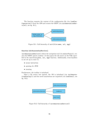
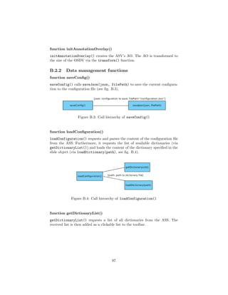
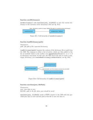
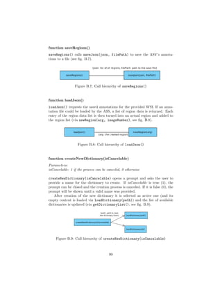
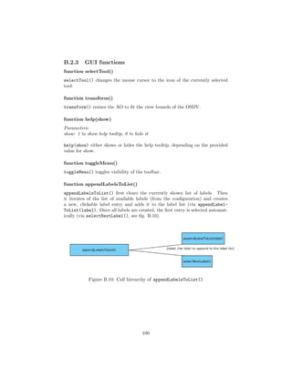
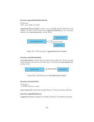
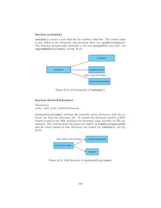
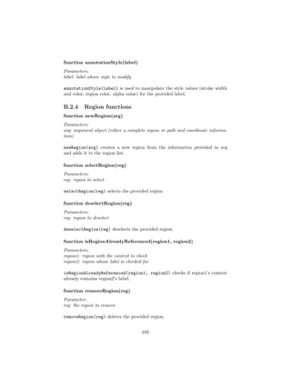
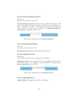
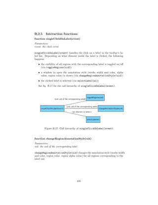
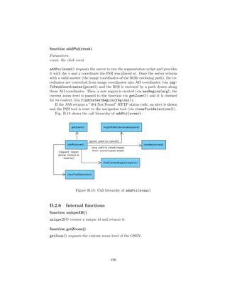
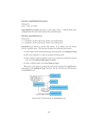
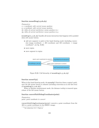
![function convertImgToPathCoordinates(point)
Parameters:
point: point coordinate to convert
convertImgToPathCoordinates(point) converts a point coordinate from the
OSDV’s image to a point coordinate in the AO.
function finishDrawingPolygon(closed)
Parameters:
closed: 1 if path should be closed, 0 otherwise
finishDrawingPolygon(closed) finishes the drawing process of a region’s path
in polygon drawing mode. If closed is true (1), the first and last segment will
be connected.
function getDistance()
getDistance() calculates the euclidian distance d between pixels pa and pb
(see eq. B.1 [74]) of a special path called ruler that is exclusively used for the
distance measurement tool.
d = (pb.x − pa.x)2 + (pb.y − pa.y)2 (B.1)
function clearToolSelection()
clearToolSelection() resets the mouse cursor to the default icon.
B.2.7 Key listener
$(document).keyup(function(e))
$(document).keyup(function(e)) resets the selected tool to the navigation
tool upon release of a hotkey (via clearToolSelection(), see fig. B.21).
Figure B.21: Call hierarchy of keyup(function(e))
109](https://image.slidesharecdn.com/5fb6f304-59ac-4e5f-8514-f4f12554de32-161019112150/85/document-112-320.jpg)
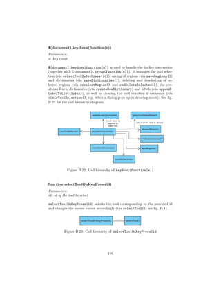
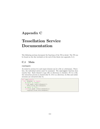
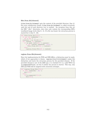
![C.2 WSI
wsi(file)
wsi(file) extracts the regions from a WSI. To do so, the provided file must
have an associated JSON file which was annotated with the dictionary provided
as argument when the TS was started (compare subsection 5.3.1).
OpenSlide is used to read the provided WSI (see line 2). The file name
is extracted from the file path (see line 3). The saved regions are loaded and
parsed via read json(path) function (see line 4).
For each parsed region, an image is extracted together with a metadata file.
If the TS was started with -t (compare tab. 5.1), tessellate wsi(slide,
slide name, region) is called. Otherwise, the BB is calculated via get
bounding box(region). If the -r parameter was provided, the BB will be ad-
justed to fit the supplied image ratio (via resize bounding box(bounding box),
see line 10 - 12). Afterwards, the BB’s position inside the baseline image of the
provided WSI is determined (see line 13). Afterwards, the size of the BB is cal-
culated for both dimension (see line 14). OpenSlide’s read region(location,
level, size) is used to access the ROI located at the specified position (the
baseline image is at level 0 [16], see line 15). The extracted image is then saved
via the save image(image, region, slide name) function.
Once every region was extracted, the OpenSlide object is closed again.
1 def wsi ( f i l e ) :
2 s l i d e = OpenSlide ( f i l e )
3 slide name = f i l e . s p l i t ( ’ / ’ ) [ −1]
4 r e g i o n s = read json ( f i l e + ’ ’ + DICTIONARY)
5
6 f o r region in r e g i o n s :
7 i f (TESSELLATE) :
8 t e s s e l l a t e w s i ( s l i d e , slide name , region )
9 e l s e :
10 bounding box = get bounding box ( region )
11 i f (RESIZE) :
12 bounding box = resize bounding box ( bounding box )
13 l o c a t i o n = ( bounding box [ ’ x min ’ ] , bounding box [ ’ y min ’ ] )
14 s i z e = ( bounding box [ ’ x max ’ ] − bounding box [ ’ x min ’ ] , bounding box
[ ’ y max ’ ] − bounding box [ ’ y min ’ ] )
15 image = s l i d e . read region ( location , 0 , s i z e )
16 save image ( image , region , slide name )
17
18 s l i d e . c l o s e ()
113](https://image.slidesharecdn.com/5fb6f304-59ac-4e5f-8514-f4f12554de32-161019112150/85/document-116-320.jpg)
![is supported(file)
is supported(file) checks if a provided file is a proprietary WSI (see subsec-
tion 2.1.2).
1 def is suppoted ( f i l e ) :
2 ext = ( f i l e . s p l i t ( ’ . ’ ) ) [ −1]
3 i f (
4 ’ b i f ’ in ext or
5 ’ mrxs ’ in ext or
6 ’ npdi ’ in ext or
7 ’ scn ’ in ext or
8 ’ svs ’ in ext or
9 ’ s v s l i d e ’ in ext or
10 ’ t i f ’ in ext or
11 ’ t i f f ’ in ext or
12 ’vms ’ in ext or
13 ’vmu ’ in ext
14 ) :
15 return 1
16 e l s e :
17 return 0
tessellate wsi(slide, slide name, region)
tessellate wsi(slide, slide name, region) realizes the approximation of
an ROI through tessellation (compare subsection 5.3.4). To do so, it acquires
the slide dimensions to calculate the amount of virtual tiles necessary to cover
the whole WSI (see line 2 - 4). Afterwards, a contour is created by iteration
over every segment of a region’s path and associating it with a virtual tile (see
line 10 - 18). The result is a contour of virtual tiles.
In the next step, the RI is created. Each pixel in the RI corresponds to a
virtual tile. Because of this relation between tiles and pixels, the created tile
contour can be used to fill in the ROI in the RI via OpenCV’s cv2.drawContours
function (see line 23). The provided parameters are:
• cv ref img: the RI
• [contour]: the list of contours to draw
• 0: which contour to draw from the provided array (0 equals all)
• (255, 255, 255): a tupel with the color in which the contour is drawn in
(white)
• -1: the stroke width of the contour (-1 equals fill)
The result is the RI. Each pixel corresponding to a virtual tile inside the
ROI is white. In the next step, the function iterates over every single pixel of
the RI and extracts the associated tile into an individual image, whenever the
corresponding pixel is white (see line 27 - 37).
After all tiles are extracted, an associated metadata file is created (see line
40).
114](https://image.slidesharecdn.com/5fb6f304-59ac-4e5f-8514-f4f12554de32-161019112150/85/document-117-320.jpg)
![1 def t e s s e l l a t e w s i ( s l i d e , slide name , region ) :
2 n ,m = s l i d e . dimensions
3 m = m / TESSELLATE[HEIGHT]
4 n = n / TESSELLATE[WIDTH]
5
6 i f SHOW:
7 ox = 999999
8 oy = 999999
9
10 contour = [ ]
11 f o r coords in region . get ( ’ imgCoords ’ ) :
12 i f SHOW:
13 i f ( coords . get ( ’ y ’ ) < oy ) : oy = coords . get ( ’ y ’ )
14 i f ( coords . get ( ’ x ’ ) < ox ) : ox = coords . get ( ’ x ’ )
15 x = i n t ( coords . get ( ’ x ’ ) / TESSELLATE[WIDTH] )
16 y = i n t ( coords . get ( ’ y ’ ) / TESSELLATE[HEIGHT] )
17 i f [ x , y ] not in contour :
18 contour . append ( [ x , y ] )
19
20 contour = np . asarray ( contour )
21 ref img = Image . new( ’RGB’ , (n ,m) )
22 cv re f im g = np . array ( ref img )
23 cv2 . drawContours ( cv ref img , [ contour ] , 0 , (255 ,255 ,255) , −1)
24 i f SHOW:
25 dbg img = Image . new( ’RGB’ , (n ,m) )
26 t i l e s = [ ]
27 f o r i in xrange (0 , m) :
28 f o r j in xrange (0 , n) :
29 px = c v re f im g [ i , j ]
30 i f ( px == [255 , 255 , 255]) . a l l () :
31 l o c a t i o n = (( j ) ∗ TESSELLATE[WIDTH] , ( i ) ∗ TESSELLATE[
HEIGHT] )
32 s i z e = TESSELLATE
33 t i l e = s l i d e . read region ( location , 0 , s i z e )
34 tile name = save image ( t i l e , region , slide name , i , j )
35 t i l e s . append ( tile name . s p l i t ( ’ / ’ ) [ −1] + ’ . jpeg ’ )
36 i f SHOW:
37 dbg img . paste ( t i l e , ( j ∗ TESSELLATE[WIDTH] − i n t ( ox ) , i ∗
TESSELLATE[HEIGHT] − i n t ( oy ) ) )
38 i f SHOW:
39 dbg img . show ()
40 save metadata ( g e n e r a t e f i l e n a m e ( region , slide name ) , region ,
t i l e s )
115](https://image.slidesharecdn.com/5fb6f304-59ac-4e5f-8514-f4f12554de32-161019112150/85/document-118-320.jpg)
![C.3 DZI
dzi(file)
dzi(file) extracts the regions from a DZI. Since OpenSlide can not be used
with DZIs, the corresponding ROI must be stitched manually. To do so, the
provided file’s DZI metadata must be parsed to access the information about
width, height, format and location of the highest resolution layer (see line 2 -
6). The saved regions are parsed with the read json(path) function (see line
7).
For each parsed region, an image is extracted together with a metadata file,
like in the WSI scenario. If the tessellation parameter was provided when Tes-
sellationService.py was called, tessellate dzi(dzi, slide name, region) is
called. Otherwise, the BB is calculated via get bounding box(region). The
tiles containing the ROI are stitched together and cropped to size in the cre-
ate image from tiles(dzi, bounding box) function. The resulting image is
saved via the save image(image, region, slide name) function (see line 10
- 15).
1 def dzi ( f i l e ) :
2 slide name = f i l e . s p l i t ( ’ / ’ ) [ −1]
3 with open ( f i l e , ’ r ’ ) as d z i f i l e :
4 content = d z i f i l e . read ()
5 root = ET. fromstring ( content )
6 dzi = { ’ t i l e s i z e ’ : i n t ( root . get ( ’ T i l e S i z e ’ ) ) , ’ width ’ : i n t ( root
[ 0 ] . get ( ’Width ’ ) ) , ’ height ’ : i n t ( root [ 0 ] . get ( ’ Height ’ ) ) , ’
t i l e s o u r c e ’ : g e t t i l e s o u r c e ( f i l e ) , ’ format ’ : root . get ( ’ Format
’ ) }
7 r e g i o n s = read json ( f i l e + ’ ’ + DICTIONARY)
8
9 f o r region in r e g i o n s :
10 i f TESSELLATE:
11 t e s s e l l a t e d z i ( dzi , slide name , region )
12 e l s e :
13 bounding box = get bounding box ( region )
14 image = c r e a t e i m a g e f r o m t i l e s ( dzi , bounding box )
15 save image ( image , region , slide name )
create image from tiles(dzi, bounding box)
create image from tiles(dzi, bounding box) stitches the tiles containing
the baseline area by utilizing the ROI’s BB.
If the TS was executed with the -r parameter (compare tab. 5.1), the BB
will be adjusted to fit the provided image ratio. This also has influence on
what tiles will be needed (see line 2 - 3). The stitching of the baseline area
is realized in get tiles from bounding box(dzi, bounding box) (see line 4).
Once the tiles are stitched, the offset of the ROI’s BB inside the stitched image
is calculated (see line 6 - 7), as well as its corners (see line 9 - 12).
This information is used to crop the stitched image to the size of the ROI’s
BB.
116](https://image.slidesharecdn.com/5fb6f304-59ac-4e5f-8514-f4f12554de32-161019112150/85/document-119-320.jpg)
![1 def c r e a t e i m a g e f r o m t i l e s ( dzi , bounding box ) :
2 i f (RESIZE) :
3 bounding box = resize bounding box ( bounding box )
4 t i l e i m a g e = g e t t i l e s f r o m b o u nd i n g b o x ( dzi , bounding box )
5
6 o f f s e t x = bounding box [ ’ x min ’ ]
7 o f f s e t y = bounding box [ ’ y min ’ ]
8
9 x min = bounding box [ ’ x min ’ ] − o f f s e t x
10 x max = bounding box [ ’ x max ’ ] − o f f s e t x
11 y min = bounding box [ ’ y min ’ ] − o f f s e t y
12 y max = bounding box [ ’ y max ’ ] − o f f s e t y
13
14 return t i l e i m a g e . crop (( x min , y min , x max , y max ) )
get tiles from bounding box(dzi, bounding box)
get tiles from bounding box(dzi, bounding box) stitches together a base-
line area based on the provided BB.
To do so, the corners of the BB are converted to tile positions (see line 2 - 5).
Then, a new image is created which will hold the tiles (see line 7). All needed
tiles are iterated in width and height and pasted to the corresponding postion
of the holding image (see line 9 - 12). The stitched image is then returned.
1 def g e t t i l e s f r o m b o u nd i n g b o x ( dzi , bounding box ) :
2 x min = bounding box [ ’ x min ’ ] / dzi [ ’ t i l e s i z e ’ ]
3 x max = bounding box [ ’ x max ’ ] / dzi [ ’ t i l e s i z e ’ ]
4 y min = bounding box [ ’ y min ’ ] / dzi [ ’ t i l e s i z e ’ ]
5 y max = bounding box [ ’ y max ’ ] / dzi [ ’ t i l e s i z e ’ ]
6
7 s t i t c h = Image . new( ’RGB’ , (( x max−x min+1) ∗ dzi [ ’ t i l e s i z e ’ ] , (
y max−y min+1) ∗ dzi [ ’ t i l e s i z e ’ ] ) )
8
9 f o r i in range ( x min , x max+1) :
10 f o r j in range ( y min , y max+1) :
11 t i l e = Image . open ( dzi [ ’ t i l e s o u r c e ’ ] + s t r ( i ) + ’ ’ + s t r ( j )
+ ’ . ’ + dzi [ ’ format ’ ] )
12 s t i t c h . paste ( t i l e , (( i − x min ) ∗ dzi [ ’ t i l e s i z e ’ ] , ( j −
y min ) ∗ dzi [ ’ t i l e s i z e ’ ] ) )
13 return s t i t c h
get tile source(file)
get tile source(file) finds the level with the highest resolution in a DZI’s
” files” directory and builds a file path based on that.
1 def g e t t i l e s o u r c e ( f i l e ) :
2 f i l e s d i r = f i l e . r e p l a c e ( ’ . dzi ’ , ’ f i l e s / ’ )
3 l a y e r s = os . l i s t d i r ( f i l e s d i r )
4 l a y e r s . remove ( ’ metadata . txt ’ )
5 l a y e r s = map( int , l a y e r s )
6 return f i l e s d i r + s t r (max( l a y e r s ) ) + ’ / ’
117](https://image.slidesharecdn.com/5fb6f304-59ac-4e5f-8514-f4f12554de32-161019112150/85/document-120-320.jpg)
![tessellate dzi(dzi, slide name, region)
tessellate dzi(dzi, slide name, region) works in the same way as tes-
sellate wsi(slide, slide name, region), except for the tile extraction (see
line 24 - 33).
As in dzi(file), a baseline image area must be stitched (see line 3). To ex-
tract a virtual tile from that stitched image, tessellate dzi(dzi, slide name,
region) crops that stitched image to the size of the current virtual tile and saves
this in an individual image.
Once all tiles are extracted, a metadata file is created (see line 39).
1 def t e s s e l l a t e d z i ( dzi , slide name , region ) :
2 bounding box = get bounding box ( region )
3 t i l e i m a g e = g e t t i l e s f r o m b o u nd i n g b o x ( dzi , bounding box )
4 o f f s e t x = bounding box [ ’ x min ’ ]
5 o f f s e t y = bounding box [ ’ y min ’ ]
6
7 n ,m = t i l e i m a g e . s i z e
8 m = m / TESSELLATE[HEIGHT]
9 n = n / TESSELLATE[WIDTH]
10
11 contour = [ ]
12 f o r coords in region . get ( ’ imgCoords ’ ) :
13 x = i n t (( coords . get ( ’ x ’ ) − o f f s e t x ) / TESSELLATE[WIDTH] )
14 y = i n t (( coords . get ( ’ y ’ ) − o f f s e t y ) / TESSELLATE[HEIGHT] )
15 i f [ x , y ] not in contour :
16 contour . append ( [ x , y ] )
17
18 contour = np . asarray ( contour )
19 ref img = Image . new( ’RGB’ , (n ,m) )
20 cv re f im g = np . array ( ref img )
21 cv2 . drawContours ( cv ref img , [ contour ] , 0 , (255 ,255 ,255) , −1)
22 i f SHOW:
23 dbg img = Image . new( ’RGB’ , t i l e i m a g e . s i z e )
24 t i l e s = [ ]
25 f o r i in xrange (0 , m) :
26 f o r j in xrange (0 , n) :
27 px = c v re f im g [ i , j ]
28 i f ( px == [255 , 255 , 255]) . a l l () :
29 t i l e = t i l e i m a g e . crop (( j ∗ TESSELLATE[WIDTH] + (
bounding box [ ’ x min ’ ] % dzi [ ’ t i l e s i z e ’ ] ) ,
30 i ∗ TESSELLATE[HEIGHT] + ( bounding box [ ’ y min ’ ] % dzi [ ’
t i l e s i z e ’ ] ) ,
31 j ∗ TESSELLATE[WIDTH] + ( bounding box [ ’ x min ’ ] % dzi [ ’
t i l e s i z e ’ ] ) + TESSELLATE[WIDTH] ,
32 i ∗ TESSELLATE[HEIGHT] + ( bounding box [ ’ y min ’ ] % dzi [ ’
t i l e s i z e ’ ] ) + TESSELLATE[HEIGHT] ) )
33 tile name = save image ( t i l e , region , slide name , i , j )
34 t i l e s . append ( tile name . s p l i t ( ’ / ’ ) [ −1] + ’ . jpeg ’ )
35 i f SHOW:
36 dbg img . paste ( t i l e , ( j ∗ TESSELLATE[WIDTH] , i ∗
TESSELLATE[HEIGHT] ) )
37 i f SHOW:
38 dbg img . show ()
39 save metadata ( g e n e r a t e f i l e n a m e ( region , slide name ) , region ,
t i l e s )
118](https://image.slidesharecdn.com/5fb6f304-59ac-4e5f-8514-f4f12554de32-161019112150/85/document-121-320.jpg)
![C.4 Utility
read json(path)
read json(path) is utilized to read a provided JSON file and parse its contents
into a python dictionary (see line 2 - 6). If an error occurred in the extraction
process, the user will be informed (see line 7 - 8).
1 def read json ( path ) :
2 try :
3 with open ( path , ’ r ’ ) as f i l e :
4 s t r = ( f i l e . read () )
5 data = json . loads ( s t r . decode ( ’ utf −8 ’ ) )
6 return data
7 except IOError :
8 print ( ’ Could not load saved annotations from ’ + path )
save metadata(name, region, *tiles)
save metadata(name, region, *tiles) is used to save the metadata to a cor-
responding extracted image.
The metadata differs slightly if the -t parameter (compare tab. 5.1) was
provided (compare tab. 5.2) at the TS’ execution. Therefore, ” tessellated” is
added to the file’s name (see line 2 - 3). If the -f parameter was provided, files
of the same name will be overwritten. Otherwise, an upwards counting, positive
integer is added in parenthesis to the file name (see line 4 - 10).
A file stream is opened and the associated region’s metadata is written into a
file (see line 12 - 19). The metadata file is encoded in UTF-8 to support special
characters.
1 def save metadata (name , region , ∗ t i l e s ) :
2 i f len ( t i l e s ) > 0:
3 name = name + ’ t e s s e l l a t e d . metadata . json ’
4 i f not FORCE:
5 cnt = 0
6 while os . path . i s f i l e (name) :
7 cnt+=1
8 name = name + ’ ( ’ + s t r ( cnt ) +’ ) ’
9 e l s e :
10 image name = name
11 name = name + ’ . metadata . json ’
12 with open (name , ’w+’ ) as f i l e :
13 data = { ’ l a b e l ’ : region . get ( ’name ’ ) , ’zoom ’ : region . get ( ’zoom ’ )
, ’ context ’ : region . get ( ’ context ’ ) }
14 i f len ( t i l e s ) > 0:
15 data [ ’ t i l e s ’ ] = t i l e s
16 e l s e :
17 data [ ’ image ’ ] = image name . s p l i t ( ’ / ’ ) [ −1] + ’ . jpeg ’
18 content = json . dumps( data , e n s u r e a s c i i=False )
19 f i l e . write ( content . encode ( ’ utf −8 ’ ) )
119](https://image.slidesharecdn.com/5fb6f304-59ac-4e5f-8514-f4f12554de32-161019112150/85/document-122-320.jpg)
![generate file name(region, slide name, *tiles)
generate file name(region, slide name, *tiles) creates a file name and
output path for the provided information. The generated file name is used for
the metadata as well as the image file.
If the -o parameter was provided (compare tab. 5.1), the supplied output
directory will be added to the file path. If the path does not exist, it is created
(see line 2 - 5). The region’s uid is added to the file name (see line 8). If the
image is tessellated into tiles (*tiles will be a non-empty tupel with the x and y
position of the tile), the position of the tile will be added to the file name (see
line 9 - 13).
When the -f parameter was not specified, an upwards counting, positive
integer will be added to the file name (see line 12 - 16). The created file name
is then returned (see line 17).
1 def g e n e r a t e f i l e n a m e ( region , slide name , ∗ t i l e s ) :
2 i f (OUTPUT) :
3 dest = OUTPUT + region [ ’name ’ ]
4 e l s e :
5 dest = region [ ’name ’ ]
6 i f not os . path . e x i s t s ( dest ) :
7 os . makedirs ( dest )
8 name = dest + ’ / ’ + slide name + ’ ’ + s t r ( region [ ’ uid ’ ] )
9 i f len ( t i l e s ) > 0:
10 f o r entry in t i l e s :
11 name += ” ” + s t r ( entry )
12 i f not FORCE:
13 cnt = 0
14 while os . path . i s f i l e (name) :
15 cnt+=1
16 name = name + ’ ( ’ + s t r ( cnt ) +’ ) ’
17 return name
save image(image, region, slide name, *tiles
save image(image, region, slide name, *tiles saves an extracted image.
The file name is generated, either for a tiled or non-tiled image (see line 2 -
5). If -r was specified (compare tab. 5.1), the image will be resized according
to the specified values with the provided interpolation method, if applicable.
Otherwise, nearest neighbor interpolation is chosen by default (see line 6 - 7).
If the grayscale conversion is activated (-g parameter, compare tab. 5.1),
the image will be converted to grayscale via the luma transform method (see
eq. 5.1 in subsection 5.3.2).
The image is then saved and the path returned (see line 11 - 14). If the
image is not tessellated, the metadata is saved automatically as well (see line
12 - 13).
120](https://image.slidesharecdn.com/5fb6f304-59ac-4e5f-8514-f4f12554de32-161019112150/85/document-123-320.jpg)
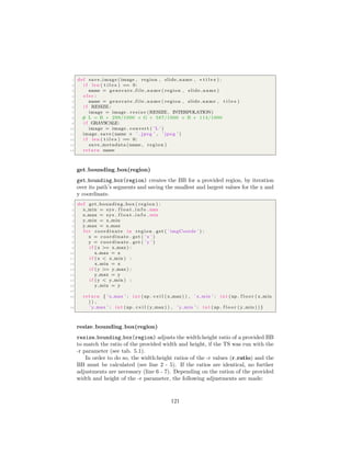
![• r ratio = 1: the BB is adjusted to a square (see line 9 - 13)
• r ratio <1: the BB must be adjusted to rectangle that is wider than high
(see line 20 - 32)
• r ratio >1: the BB must be adjusted to rectangle that is higher than
wide (see line 33 - 45)
If the BB is smaller than the specified values after the adjustment, the BB
is scaled up to match the specified values via scale bounding box(bounding ,
scale) (see line 48 - 55). If the scaling process creates a negative value for
either one of the minimum values, the BB is moved in such a way, that the
negative value will turn to 0 (see line 57 - 64).
1 def resize bounding box ( bounding box ) :
2 r r a t i o = RESIZE [WIDTH] / f l o a t (RESIZE [HEIGHT] )
3 bb width = f l o a t ( bounding box [ ’ x max ’ ] − bounding box [ ’ x min ’ ] )
4 bb height = f l o a t ( bounding box [ ’ y max ’ ] − bounding box [ ’ y min ’ ] )
5 bb rat io = bb width / bb height
6 i f r r a t i o == bb rat io :
7 return bounding box
8 e l s e :
9 i f r r a t i o == 1:
10 # target i s square
11 s1 = bb height / bb width
12 s2 = bb width / bb height
13 scaled = min( bb width , bb height ) ∗ max( s1 , s2 ) − min(
bb width , bb height )
14 i f ( bb width > bb height ) :
15 bounding box [ ’ y min ’ ] −= i n t (np . f l o o r ( scaled /2) )
16 bounding box [ ’ y max ’ ] += i n t (np . c e i l ( scaled /2) )
17 e l s e :
18 bounding box [ ’ x min ’ ] −= i n t (np . f l o o r ( scaled /2) )
19 bounding box [ ’ x max ’ ] += i n t (np . c e i l ( scaled /2) )
20 e l i f r r a t i o < 1:
21 # target i s higher than wide
22 h s = 1 / r r a t i o
23 i f bb height > ( bb width ∗ h s ) :
24 # adjust width :
25 w new = ( bb height / h s ) − bb width
26 bounding box [ ’ x min ’ ] −= i n t (np . f l o o r (w new/2) )
27 bounding box [ ’ x max ’ ] += i n t (np . c e i l (w new/2) )
28 e l s e :
29 # adjust height :
30 h new = h s ∗ bb width − bb height
31 bounding box [ ’ y min ’ ] −= i n t (np . f l o o r ( h new /2) )
32 bounding box [ ’ y max ’ ] += i n t (np . c e i l ( h new /2) )
33 e l s e :
34 # target i s wider than high
35 w s = r r a t i o
36 i f bb width > ( bb height ∗ w s ) :
37 # adjust height
38 h new = ( bb width / w s ) − bb height
39 bounding box [ ’ y min ’ ] −= i n t (np . f l o o r ( h new /2) )
40 bounding box [ ’ y max ’ ] += i n t (np . c e i l ( h new /2) )
41 e l s e :
122](https://image.slidesharecdn.com/5fb6f304-59ac-4e5f-8514-f4f12554de32-161019112150/85/document-125-320.jpg)
![42 # adjust width :
43 w new = w s ∗ bb height − bb width
44 bounding box [ ’ x min ’ ] −= i n t (np . f l o o r (w new/2) )
45 bounding box [ ’ x max ’ ] += i n t (np . c e i l (w new/2) )
46
47 # check i f bb i s big enough
48 bb width = f l o a t ( bounding box [ ’ x max ’ ] − bounding box [ ’ x min ’ ] )
49 i f bb width < RESIZE [WIDTH] :
50 s = RESIZE [WIDTH] / bb width
51 bounding box = scale bounding box ( bounding box , s )
52 bb height = f l o a t ( bounding box [ ’ y max ’ ] − bounding box [ ’ y min ’
] )
53 i f bb height < RESIZE [HEIGHT ] :
54 s = RESIZE [HEIGHT] / bb height
55 bounding box = scale bounding box ( bounding box , s )
56
57 i f ( bounding box [ ’ y min ’ ] < 0) :
58 d i f = bounding box [ ’ y min ’ ] ∗ (−1)
59 bounding box [ ’ y min ’ ] += d i f
60 bounding box [ ’ y max ’ ] += d i f
61 i f ( bounding box [ ’ x min ’ ] < 0) :
62 d i f = bounding box [ ’ x min ’ ] ∗ (−1)
63 bounding box [ ’ x min ’ ] += d i f
64 bounding box [ ’ x max ’ ] += d i f
65
66 return bounding box
scale bounding box(bounding , scale)
scale bounding box(bounding , scale) scale a provided BB by the provided
scale in height and width. The ROI stays in the center of the BB when scaling
up.
1 def scale bounding box ( bounding box , s c a l e ) :
2 bb width = f l o a t ( bounding box [ ’ x max ’ ] − bounding box [ ’ x min ’ ] )
3 add w = ( bb width ∗ s c a l e ) − bb width
4 bounding box [ ’ x min ’ ] −= i n t (np . f l o o r ( add w /2) )
5 bounding box [ ’ x max ’ ] += i n t (np . c e i l ( add w /2) )
6
7 bb height = f l o a t ( bounding box [ ’ y max ’ ] − bounding box [ ’ y min ’ ] )
8 add h = ( bb height ∗ s c a l e ) − bb height
9 bounding box [ ’ y min ’ ] −= i n t (np . f l o o r ( add h /2) )
10 bounding box [ ’ y max ’ ] += i n t (np . c e i l ( add h /2) )
11
12 return bounding box
123](https://image.slidesharecdn.com/5fb6f304-59ac-4e5f-8514-f4f12554de32-161019112150/85/document-126-320.jpg)
![Bibliography
[1] A. Madabhushi A. Janowczyk. Deep learning for digital pathology image
analysis: A comprehensive tutorial with selected use cases. J Pathol Inform,
7(29), July 2016.
[2] L. Fei-Fei A. Karpathy. Deep Visual-Semantic Alignments for Generating
Image Descriptions. Department of Computer Science, Standford Univer-
sity, 2015. http://cs.stanford.edu/people/karpathy/cvpr2015.pdf.
[3] AgileLoad. Performance symptoms and issues. http://www.
agileload.com/performance-testing/performance-testing-
methodology/performance-symptoms-and-issues. Accessed:
24.08.2016.
[4] Neuroanatomy Applied and Theoretical (NAAT). Microdraw. http://
microdraw.pasteur.fr/index.html. Accessed: 23.08.2016.
[5] R. Berta. deepzoom. http://search.cpan.org/~drrho/Graphics-DZI-
0.05/script/deepzoom. Accessed: 22.08.2016.
[6] G. Brandl. Python Web Server Gateway Interface v1.0, June 2016. https:
//hg.python.org/peps/file/tip/pep-0333.txt.
[7] J. Bugwadia. Microservices: Five architectural constraints. http:
//www.nirmata.com/2015/02/microservices-five-architectural-
constraints/, February 2015. Accessed: 12.08.2016.
[8] D. Siganos C. Stergiou. Neural networks. Technical report, Imperial College
London, 1995. https://www.doc.ic.ac.uk/~nd/surprise_96/journal/
vol4/cs11/report.html#Conclusion.
[9] L. Dykes C. Ullmann. Beginning Ajax. Wiley Publishing, Inc.,
2007. http://crypto.cs.mcgill.ca/~simonpie/webdav/ipad/
EBook/Programmation/Beginning%20Ajax%20(Programmer%20to%
20Programmer).pdf.
[10] A. Clifford. The Math Book: From Pythagoras to the 57th Dimension, 250
Milestones in the History of Mathematics. Sterling, 2007.
124](https://image.slidesharecdn.com/5fb6f304-59ac-4e5f-8514-f4f12554de32-161019112150/85/document-127-320.jpg)
![[11] T. Cornish. An introduction to digital whole slide imaging and whole slide
image analysis. http://www.hopkinsmedicine.org/mcp/PHENOCORE/
CoursePDFs/2013/13%2019%20Cornish%20Digital%20Path.pdf, July
2013. Accessed: 12.04.2016.
[12] T. Cramer. The international image interoperability frame-
work (iiif): Laying the foundation for common services, inte-
grated resources and a marketplace of tools for scholars world-
wide. https://www.cni.org/topics/information-access-
retrieval/international-image-interoperability-framework,
December 2011. Accessed: 18.08.2016.
[13] J. Cupitt. Vips. http://www.vips.ecs.soton.ac.uk/index.php?title=
VIPS. Accessed: 25.05.2016.
[14] G. Seeman D. Bourg. AI for Game Developers. O’Reilly, 2004.
[15] M. Marcellin D. Taubmann. JPEG 2000: Image compression fundamentals,
standards and practice. Kluwer Academic Publishers, 2001.
[16] Working Group 26. Pathology DICOM Standards Committee. Digital
imaging and communications in medicine (dicom), supplement 145: Whole
slide microscopic image iod and sop classes, August 2010.
[17] digitalpreservation. Bigtiff. http://www.digitalpreservation.gov/
formats/fdd/fdd000328.shtml. Accessed: 20.08.2016.
[18] digitalpreservation. Tiff. http://www.digitalpreservation.gov/
formats/fdd/fdd000237.shtml. Accessed: 20.08.2016.
[19] D. Doubrovkine. Dzt. https://github.com/dblock/dzt. Accessed:
22.08.2016.
[20] S. Eddins. Tiff, bigtiff, and blockproc. http://blogs.mathworks.com/
steve/2013/08/07/tiff-bigtiff-and-blockproc/, August 2013.
[21] A. Goode et al. Openslide: A vendor-neutral software foundation for digital
pathology. J pathol inform, 4(1), September 2013. http://download.
openslide.org/docs/JPatholInform_2013_4_1_27_119005.pdf.
[22] D. Wilbur et al. Whole-slide imaging digital pathology as a plat-
form for teleconsultation. Arch Pathol Lab Med, 133(12), December
2009. http://www.ncbi.nlm.nih.gov/pmc/articles/PMC3694269/pdf/
nihms-486265.pdf.
[23] E. Tseytlin et al. Wsi zoomviewer. http://www.pathologyinformatics.
com/sites/default/files/archives/2014/Day2/20140514%201120%
20-%20WSI%20Zoom%20Viewer.pdf, 2014. Accessed: 22.08.2016.
125](https://image.slidesharecdn.com/5fb6f304-59ac-4e5f-8514-f4f12554de32-161019112150/85/document-128-320.jpg)
![[24] H. Guedri et al. Reconstruction of the human retinal blood vessels by
fractal interpolation. Journal of Theoretical and Applied Information Tech-
nology, 83(2), January 2016. http://www.jatit.org/volumes/Vol83No2/
9Vol83No2.pdf.
[25] H. Sharma et al. Robust segmentation of overlapping cells in histopathol-
ogy specimens using parallel seed detection and repulsive level set. IEEE
Transactions on Biomedical Engineering, 59(3), March 2012.
[26] H. Sharma et al. Deep convolutional neural networks for histological im-
age analysis in gastric cancer whole slide images. Computerized Medical
Imaging and Graphics, December 2016.
[27] M. Appleby et al. Iiif image api 2.0. http://iiif.io/api/image/2.0/.
Accessed: 18.08.2016.
[28] M. Egmonst-Petersen et al. Image processing with neural networks
- a review. Pattern Regcognition, 35, October 2002. https://www.
researchgate.net/publication/220603536_Image_processing_with_
neural_networks_-_a_review_Pattern_Recogn_352279C2301.
[29] M. Frosterus et al. Extending ontologies with free keywords in a collab-
orative annotation environment. Technical report, University of Helsinki,
2010. http://ceur-ws.org/Vol-809/paper-02.pdf.
[30] N. Farahanil et al. Whole slide imaging in pathology: advantages, limi-
tations, and emerging perspectives. Pathology and Laboratory Medicine
International, 7, June 2015. https://www.dovepress.com/whole-slide-
imaging-in-pathology-advantages-limitations-and-emerging-p-
peer-reviewed-fulltext-article-PLMI#ref10.
[31] P. Th´evanez et al. Image interpolation and resampling. Handbook of Med-
ical Imaging, Processing and Analysis, 2000. http://bigwww.epfl.ch/
publications/thevenaz9901.pdf.
[32] R. Harvey et al. A neural network architecture for general image recogni-
tion. The Lincoln Library Journal, 4(2), 1991. https://www.ll.mit.edu/
publications/journal/pdf/vol04_no2/4.2.5.neuralnetwork.pdf.
[33] R. Singh et al. Standardization in digital pathology: Supple-
ment 145 of the dicom standards. J pathol inform, 2(23), March
2011. http://www.jpathinformatics.org/temp/JPatholInform2123-
3144928_084409.pdf.
[34] S. Doyle et al. A boosted bayesian multi-resolution classifier for prostate
cancer detection from digitized needle biopsies. Transactions on Biomedical
Engineering, June 2010. https://www.researchgate.net/publication/
44695140_A_Boosted_Bayesian_Multiresolution_Classifier_for_
Prostate_Cancer_Detection_From_Digitized_Needle_Biopsies.
126](https://image.slidesharecdn.com/5fb6f304-59ac-4e5f-8514-f4f12554de32-161019112150/85/document-129-320.jpg)
![[35] S. Park et al. Digital imaging in pathology. Clin Lab Med, 4(32), December
2012.
[36] S. Wienert et al. Detection and segmentation of cell nuclei in virtual mi-
croscopy images: A minimum-model approach. Scientific Reports, 2(503),
Juli 2012. http://www.ncbi.nlm.nih.gov/pmc/articles/PMC3694269/
pdf/nihms-486265.pdf.
[37] R. Fielding. Architectural Styles and the Design of Network-based Software
Architectures. PhD thesis, University of Carolina, 2000. http://www.ics.
uci.edu/~fielding/pubs/dissertation/top.htm.
[38] Flask. Flask user guide. http://flask.pocoo.org/docs/0.11/. Accessed:
24.08.2016.
[39] National Institute for Standards and Technology. Pyramidio. https://
github.com/usnistgov/pyramidio. Accessed: 22.08.2016.
[40] Open Source Geospatial Foundation. Tile map service specification. http:
//wiki.osgeo.org/wiki/Tile_Map_Service_Specification. Accessed:
26.04.2016.
[41] OpenStreetMap Foundation. Openstreetmap homepage. http://www.
openstreetmap.org/about. Accessed: 18.08.2016.
[42] L. Fuller. sharp homepage. http://sharp.dimens.io/en/stable/. Ac-
cessed: 22.08.2016.
[43] A. Kaebler G. Bradski. Learning OpenCV. O’Reilly, 2008.
[44] D. Gasienica. Vips. https://github.com/zoomhub/zoomhub. Accessed:
22.08.2016.
[45] I. Gilman. Openseadragon. http://openseadragon.github.io/
examples/creating-zooming-images/. Accessed: 26.04.2016.
[46] IIIF. Internation image interoperability framework homepage. http://
iiif.io. Accessed: 18.08.2016.
[47] ImageMagick. Imagemagick: Formats. http://www.imagemagick.org/
script/formats.php. Accessed: 22.08.2016.
[48] Optimus Information Inc. Open-source vs. proprietary software, pros and
cons. http://www.optimusinfo.com/downloads/white-paper/open-
source-vs-proprietary-software-pros-and-cons.pdf, 2015. Ac-
cessed: 16.08.2016.
[49] Radiocommunication Sector International Telecommunication Union. Rec-
ommendation itu-r bt.601-4 encoding parameters of digital television
for studios. http://www-inst.eecs.berkeley.edu/~cs150/Documents/
ITU601.PDF, 1998.
127](https://image.slidesharecdn.com/5fb6f304-59ac-4e5f-8514-f4f12554de32-161019112150/85/document-130-320.jpg)
![[50] intoPix. Everything you always wanted to know about jpeg 2000. http:
//www.intopix.com/pdf/JPEG%202000%20Handbook.pdf, 2008.
[51] K. Martinez J. Cupitt. Vips: an image processing system for large images.
Proc. SPIE, 2663:19 – 28, 1996. http://eprints.soton.ac.uk/252227/
1/vipsspie96a.pdf.
[52] K. Martinez J. Cupitt. Vips - a highly tuned image processing software
architecture. In IEEE International Conference on Image Processing, pages
574 – 577, September 2005. http://eprints.soton.ac.uk/262371/.
[53] K. Martinez J. Cupitt. Nucleus modelling and segmentation in cell clusters.
Mathematics in Industry, 15:217 – 222, May 2010.
[54] J. Puckey J. Lehni. Paper.js homepage. http://paperjs.org/about/.
Accessed: 28.08.2016.
[55] M. Fowler J.Lewis. Microservices, a definition of this new architec-
tural term. http://martinfowler.com/articles/microservices.html#
footnote-etymology, March 2014. Accessed: 12.08.2016.
[56] JPEG. Overview of jpeg 2000. https://jpeg.org/jpeg2000/. Accessed:
18.08.2016.
[57] jQuery Foundation. jquery browser support. https://jquery.com/
browser-support/. Accessed: 28.08.2016.
[58] jQuery Foundation. jquery homepage. https://jquery.com/. Accessed:
28.08.2016.
[59] A. Kesteren. Cross-Origin Resource Sharing: W3C Recommendation 16
January 2014, January 2014. https://www.w3.org/TR/cors/#cross-
origin-request.
[60] D. Kriesel. A Brief Introduction to Neural Networks, 2007. http://www.
dkriesel.com/en/science/neural_networks.
[61] D. Liu. A review of computer vision segmentation algorithms. Technical
report, University of Washington, 2012. https://homes.cs.washington.
edu/~bilge/remote.pdf.
[62] R. Joshi M. Rabbani. An overview of the jpeg2000 still image compression
standard. Signal Processing Image Communication, 17(3), 2002. https:
//www.csd.uoc.gr/~hy471/bibliography/jpeg2000.pdf.
[63] Mozilla Developer Network (MDN). Same-origin policy for file:
Uris. https://developer.mozilla.org/en-US/docs/Same-origin_
policy_for_file:_URIs. Accessed: 22.08.2016.
[64] Microsoft. Deep zoom file format overview. https://msdn.microsoft.
com/en-us/library/cc645077(v=vs.95).aspx. Accessed: 17.08.2016.
128](https://image.slidesharecdn.com/5fb6f304-59ac-4e5f-8514-f4f12554de32-161019112150/85/document-131-320.jpg)
![[65] K. Mulka. Gmap uploader tiler. https://github.com/mulka/tiler. Ac-
cessed: 22.08.2016.
[66] College of American Pathologists. Sample emplyment contract for a
pathologist. http://www.cap.org/ShowProperty?nodePath=/UCMCon/
Contribution%20Folders/WebContent/pdf/pm-sample-employment-
contract.pdf. Accessed: 22.08.2016.
[67] OpenSlide. Openslide format documentation. http://openslide.org/.
Accessed: 16.08.2016.
[68] J. Riggins. Microservices architecture: The good, the bad, and what
you could be doing better. http://nordicapis.com/microservices-
architecture-the-good-the-bad-and-what-you-could-be-doing-
better/, April 2015. Accessed: 12.08.2016.
[69] R. Rojas. Neural Networks - A Systematic Introduction. Springer-Verlag,
1996. https://page.mi.fu-berlin.de/rojas/neural/.
[70] F. Rosenblatt. The perceptron: a probabilistic model for information
storage and organization in the brain. Psychological Review, 65(6), 1958.
http://www.ling.upenn.edu/courses/cogs501/Rosenblatt1958.pdf.
[71] D. Shiffman. The Nature of Code. D. Shiffman, 2012. http://
natureofcode.com/book/chapter-10-neural-networks/.
[72] S. Smith. The Scientist and Engineer’s Guide to Digital Signal Processing.
California Technical Publishing, 1997. http://www.dspguide.com/ch26/
4.htm.
[73] The Internet Society. Hypertext transfer protocol – http/1.1. https:
//www.w3.org/Protocols/rfc2616/rfc2616.html, 1999. Accessed:
26.08.2016.
[74] G. Strang. Introduction to Linear Algebra. Springer, 2003.
[75] US San Diego Health System. Confidentiality agreement. https:
//health.ucsd.edu/about/volunteer/Documents/Confidentiality%
20Agreement%20D214.pdf. Accessed: 22.08.2016.
[76] G. Toussaint. Solving geometric problems with the rotating calipers.
Proceedings of IEEE MELECON’83, May 1983. https://www.cs.
swarthmore.edu/~adanner/cs97/s08/pdf/calipers.pdf.
[77] J. David V. Shereena. Content based image retrieval: Classification using
neural networks. The International Journal of Multimedia & Its Applica-
tions, 6(5), October 2014.
[78] S. van der Walt et al. The numpy array: A structure for efficient numerical
computation. Computing in Science & Engineering, 13(2), March 2011.
http://ieeexplore.ieee.org/document/5725236/?arnumber=5725236.
129](https://image.slidesharecdn.com/5fb6f304-59ac-4e5f-8514-f4f12554de32-161019112150/85/document-132-320.jpg)
![[79] E. Wolff. Microservices Primer. innoQ, January 2016. https://leanpub.
com/microservices-primer/read.
130](https://image.slidesharecdn.com/5fb6f304-59ac-4e5f-8514-f4f12554de32-161019112150/85/document-133-320.jpg)
![List of Figures
1.1 Example results of the in [2] introduced model (source: http:
//cs.stanford.edu/people/karpathy/deepimagesent/) . . . . 5
2.1 DICOMs image pyramid (source: [33]) . . . . . . . . . . . . . . . 8
2.2 DZI pyramid model example (source: [64]) . . . . . . . . . . . . . 12
2.3 Example of iiif request (source:http://www.slideshare.net/Tom-
Cramer/iiif-international-image-interoperability-framework-
dlf2012?ref=https://www.diglib.org/forums/2012forum/transcending-
silos-leveraging-linked-data-and-open-image-apis-for-
collaborative-access-to-digital-facsimiles/) . . . . . . . 13
2.4 Results of IIIF request with different values for region parameter
(source: [27]) . . . . . . . . . . . . . . . . . . . . . . . . . . . . . 15
2.5 Results of IIIF request with different values for size parameter
(source: [27]) . . . . . . . . . . . . . . . . . . . . . . . . . . . . . 15
2.6 Neuron in a BNN (source: [71]) . . . . . . . . . . . . . . . . . . . 18
2.7 Exemplary NN (source: [71]) . . . . . . . . . . . . . . . . . . . . 19
2.8 Perceptron by Rosenblatt (source: [71]) . . . . . . . . . . . . . . 20
2.9 Examples for linearly separable problems (source: [71]) . . . . . . 21
2.10 Examples for non-linearly separable problems (source: [71]) . . . 21
2.11 NN with multiple layers (source: http://docs.opencv.org/2.
4/_images/mlp.png) . . . . . . . . . . . . . . . . . . . . . . . . 22
2.12 Activity diagram of the process chain . . . . . . . . . . . . . . . 27
2.13 Visualization of the Conversion Service . . . . . . . . . . . . . . . 28
2.14 Visualization of the Annotation Service . . . . . . . . . . . . . . 28
2.15 Visualization of the Tessellation Service . . . . . . . . . . . . . . 29
3.1 Content of input directory . . . . . . . . . . . . . . . . . . . . . . 38
4.1 Activity diagram of ASS and ASV . . . . . . . . . . . . . . . . . 42
4.2 Example of context regions (B, C are context of A; A, C are
context of B; A, B are context of C; D has no context region) . . 44
4.3 Microdraw GUI with opened WSI . . . . . . . . . . . . . . . . . 45
131](https://image.slidesharecdn.com/5fb6f304-59ac-4e5f-8514-f4f12554de32-161019112150/85/document-134-320.jpg)
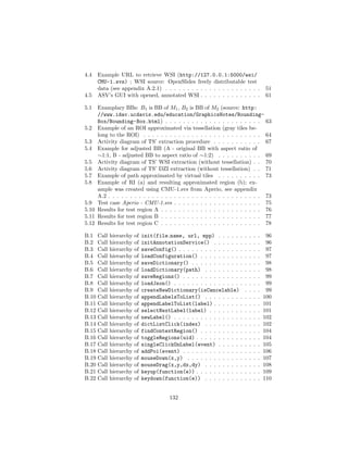

![List of Tables
2.1 File formats by vendor . . . . . . . . . . . . . . . . . . . . . . . . 9
2.2 Valid values for region parameter (source: [27]) . . . . . . . . . . 14
2.3 Valid values for size parameter (source: [27]) . . . . . . . . . . . 16
3.1 File formats by vendor . . . . . . . . . . . . . . . . . . . . . . . . 30
3.2 Overview of conversion options for zooming image formats (source:
[45]) . . . . . . . . . . . . . . . . . . . . . . . . . . . . . . . . . . 31
3.3 Options for deepzoom.py . . . . . . . . . . . . . . . . . . . . . . . 32
3.4 Options for VIPS . . . . . . . . . . . . . . . . . . . . . . . . . . . 35
3.5 Results of Conversion Service Test . . . . . . . . . . . . . . . . . 38
4.1 Available converters in Flask (source: [38]) . . . . . . . . . . . . . 47
4.2 ASS’ URL-function binding overview . . . . . . . . . . . . . . . . 47
4.3 DZG parameters (source: [67]) . . . . . . . . . . . . . . . . . . . 48
4.4 Description of get tile(level, address) parameters (source:
[67]) . . . . . . . . . . . . . . . . . . . . . . . . . . . . . . . . . . 49
4.5 Configurable parameters in configuration.json . . . . . . . . . . . 50
4.6 Parameters for as server.py . . . . . . . . . . . . . . . . . . . . . 51
4.7 Overview of used options in OSDV constructor (source: [45]) . . 55
4.8 Class diagram of the region class . . . . . . . . . . . . . . . . . . 59
5.1 Optional parameters for the TS . . . . . . . . . . . . . . . . . . . 66
5.2 Metadata information . . . . . . . . . . . . . . . . . . . . . . . . 68
5.3 File name patterns of generated output . . . . . . . . . . . . . . 69
5.4 Test cases for the TS . . . . . . . . . . . . . . . . . . . . . . . . . 74
5.5 Test-result correspondence . . . . . . . . . . . . . . . . . . . . . . 75
6.1 Correspondence of objectives, chapters and tools . . . . . . . . . 79
A.1 Services with their disc paths and repository URLs . . . . . . . . 83
A.2 Aperio data set (source: http://openslide.cs.cmu.edu/download/
openslide-testdata/Aperio/) . . . . . . . . . . . . . . . . . . 84
A.3 Generic Tiled tiff data set (source: http://openslide.cs.cmu.
edu/download/openslide-testdata/Generic-TIFF/) . . . . . . 84
134](https://image.slidesharecdn.com/5fb6f304-59ac-4e5f-8514-f4f12554de32-161019112150/85/document-137-320.jpg)