Applying Machine Learning Techniques to Revenue Management

Université de Tunis
Institut Supérieur de Gestion
MÉMOIRE DE MASTER RECHERCHE
Spécialité
Sciences et Techniques de l’Informatique Décisionnelle (STID)
Option
Informatique et Gestion de la Connaissance (IGC)
Applying Machine Learning Techniques
to Revenue Management
Multisided Platform dedicated to Restaurants Reservations
Ahmed BEN JEMIA
Soutenu le 27 Novembre 2020, devant le jury composé de:
Zied ELOUEDI Professeur, ISG Tunis Président
Lilia REJEB Maitre assistant, ISG Tunis Rapporteur
Nahla BEN AMOR Professeur, ISG Tunis Directeur du mémoire
LAboratoire de Recherche Opérationnelle de DÉcision et de Contrôle de Processus (LARODEC)
Année universitaire 2019/2020

Acknowledgments
The timely and successful completion of the research paper could hardly be possible
without the helps and supports from a lot of individuals. I will take this opportunity to
thank all of them who helped me either directly or indirectly during this important work.
First of all, I wish to express my sincere gratitude and due respect to my academic
supervisor, Ms. Nahla BEN AMOR, Professor at ISG Tunis. I am immensely grateful
to her for his valuable guidance, continuous encouragements and positive supports which
helped me a lot during the period of this work. I would like to appreciate her for always
showing keen interest in my queries and providing important suggestions.
I am also grateful to Mr. Ahmed TAKTAK, for your monitoring, your availability and
your encouragement all along the realization of this work.
I owe a lot to my family for their constant love and support. They have always encour-
aged me to think positively and independently, which really matter in my life. I would
like to thank them warmly and share this moment of happiness with them.
I also express whole hearted thanks to my friends and classmates for their care and
moral supports. The moments I spent with them during the class sessions will always
remain a happy memory for the rest of my life.
Finally, I am also grateful to all the teaching staﬀ and members of the LARODEC
laboratory of ISG TUNIS, for their selﬂess help that I have obtained whenever necessary
in my work.
Ahmed BEN JEMIA
i

Contents
Introduction 1
1 Fundamentals of Yield and Revenue Management 4
1.1 Introduction . . . . . . . . . . . . . . . . . . . . . . . . . . . . . . . . . 4
1.2 Yield management . . . . . . . . . . . . . . . . . . . . . . . . . . . . . 5
1.2.1 Applications of yield management . . . . . . . . . . . . . . . . . 6
1.2.2 Yield management system . . . . . . . . . . . . . . . . . . . . . 6
1.3 Revenue management . . . . . . . . . . . . . . . . . . . . . . . . . . . . 8
1.3.1 Restaurant revenue management . . . . . . . . . . . . . . . . . . 8
1.3.2 Revenue management system . . . . . . . . . . . . . . . . . . . 11
1.4 Yield management forecasting methods . . . . . . . . . . . . . . . . . . 12
1.4.1 Time series analysis . . . . . . . . . . . . . . . . . . . . . . . . 13
1.4.2 Regression analysis . . . . . . . . . . . . . . . . . . . . . . . . . 17
1.5 Conclusion . . . . . . . . . . . . . . . . . . . . . . . . . . . . . . . . . 19
2 Yield Management beyond Machine Learning 20
2.1 Introduction . . . . . . . . . . . . . . . . . . . . . . . . . . . . . . . . . 20
2.2 Problem statement . . . . . . . . . . . . . . . . . . . . . . . . . . . . . 21
2.3 Machine learning algorithms for regression . . . . . . . . . . . . . . . . 22
ii

CONTENTS iii
2.3.1 Simple linear regression . . . . . . . . . . . . . . . . . . . . . . 23
2.3.2 Decision trees . . . . . . . . . . . . . . . . . . . . . . . . . . . . 25
2.3.3 Random forests (RF) . . . . . . . . . . . . . . . . . . . . . . . . 28
2.3.4 Gradient boosted decision trees (GBDT) . . . . . . . . . . . . . . 31
2.3.5 K-Nearest Neighbors (K-NN) . . . . . . . . . . . . . . . . . . . 34
2.3.6 Stochastic gradient descent (SGD) . . . . . . . . . . . . . . . . . 35
2.4 Forecast performance measures . . . . . . . . . . . . . . . . . . . . . . . 37
2.5 Conclusion . . . . . . . . . . . . . . . . . . . . . . . . . . . . . . . . . 39
3 Experimental study 40
3.1 Introduction . . . . . . . . . . . . . . . . . . . . . . . . . . . . . . . . . 40
3.2 Experimental protocol . . . . . . . . . . . . . . . . . . . . . . . . . . . 41
3.2.1 Data description . . . . . . . . . . . . . . . . . . . . . . . . . . 41
3.2.2 Data cleaning . . . . . . . . . . . . . . . . . . . . . . . . . . . . 43
3.2.3 Data exploration . . . . . . . . . . . . . . . . . . . . . . . . . . 44
3.2.4 Feature relations . . . . . . . . . . . . . . . . . . . . . . . . . . 51
3.2.5 Processing weather data . . . . . . . . . . . . . . . . . . . . . . 55
3.2.6 Feature engineering . . . . . . . . . . . . . . . . . . . . . . . . . 60
3.2.7 Feature importance . . . . . . . . . . . . . . . . . . . . . . . . . 61
3.2.8 Time series analysis . . . . . . . . . . . . . . . . . . . . . . . . 63
3.3 Experimental results . . . . . . . . . . . . . . . . . . . . . . . . . . . . 69
3.4 Towards Tunisian data . . . . . . . . . . . . . . . . . . . . . . . . . . . 71
3.5 Conclusion . . . . . . . . . . . . . . . . . . . . . . . . . . . . . . . . . 71
Conclusion and future works 72
Appendix 73

CONTENTS iv
A Statistical methods for forecasting 74
A.1 Introduction . . . . . . . . . . . . . . . . . . . . . . . . . . . . . . . . . 74
A.2 Stationary Analysis . . . . . . . . . . . . . . . . . . . . . . . . . . . . . 74
A.3 SARIMA models . . . . . . . . . . . . . . . . . . . . . . . . . . . . . . 75
A.4 SARIMAX models . . . . . . . . . . . . . . . . . . . . . . . . . . . . . 76
A.5 BSTS models . . . . . . . . . . . . . . . . . . . . . . . . . . . . . . . . 77
A.6 Conclusion . . . . . . . . . . . . . . . . . . . . . . . . . . . . . . . . . 77

List of Figures
1.1 The architecture of a yield management system . . . . . . . . . . . . . . 8
1.2 Revenue management system . . . . . . . . . . . . . . . . . . . . . . . . 12
2.1 Forecasting model for visitors . . . . . . . . . . . . . . . . . . . . . . . 21
2.2 Machine learning process chart for forecasting . . . . . . . . . . . . . . . 22
2.3 Schematic of machine learning . . . . . . . . . . . . . . . . . . . . . . . 23
2.4 Visitors vs reservations with simple linear regression algorithm . . . . . . 25
2.5 Application of regression tree with the CART method . . . . . . . . . . . 28
2.6 Individual estimators (trees) learnt by random forest applied on our data
set. Each estimator is a binary regression tree with maximal depth = 3. . . 30
2.7 The regression tree found by XGB Regressor (GBDT) . . . . . . . . . . 33
3.1 PDF of average visitors per restaurant . . . . . . . . . . . . . . . . . . . 45
3.2 Boxplot of average visitors per restaurant . . . . . . . . . . . . . . . . . 46
3.3 Visitors by day of the week . . . . . . . . . . . . . . . . . . . . . . . . . 46
3.4 Average visitors each day of week . . . . . . . . . . . . . . . . . . . . . 47
3.5 Average visitors each month . . . . . . . . . . . . . . . . . . . . . . . . 47
3.6 PDF of average visitors reservations per restaurant . . . . . . . . . . . . 48
3.7 Boxplot of average visitors reservations per restaurant . . . . . . . . . . . 48
3.8 Genre wise restaurant market share . . . . . . . . . . . . . . . . . . . . . 49
v

LIST OF FIGURES vi
3.9 Description of the date info ﬁle . . . . . . . . . . . . . . . . . . . . . . . 50
3.10 Plot of train and test data sets . . . . . . . . . . . . . . . . . . . . . . . . 51
3.11 Relation between visitors and reservations . . . . . . . . . . . . . . . . . 51
3.12 Hourly visitors behaviour . . . . . . . . . . . . . . . . . . . . . . . . . . 52
3.13 Analysis of the time between the reservation and the visit to the restaurant 52
3.14 Total visitors by air genre name . . . . . . . . . . . . . . . . . . . . . . 53
3.15 Reserve visitors by genre . . . . . . . . . . . . . . . . . . . . . . . . . . 54
3.16 Average visitors on holidays and non-holidays . . . . . . . . . . . . . . . 54
3.17 Average temperature each day of week . . . . . . . . . . . . . . . . . . . 58
3.18 Average temperature each month . . . . . . . . . . . . . . . . . . . . . . 59
3.19 The impact of weather factors on visitors . . . . . . . . . . . . . . . . . . 59
3.20 Feature importance (top 20 features) . . . . . . . . . . . . . . . . . . . . 62
3.21 Feature selection using RFECV for XGBRegressor . . . . . . . . . . . . 63
3.22 Structural diﬀerence detected from 110 to 130 . . . . . . . . . . . . . . . 64
3.23 ACF, PACF and residuals plots for ARIMA . . . . . . . . . . . . . . . . 65
3.24 ACF, PACF and residuals plots for SARIMAX . . . . . . . . . . . . . . . 67
3.25 ACF, PACF and residuals plots for BSTS . . . . . . . . . . . . . . . . . . 68
3.26 Residuals plots for BSTS . . . . . . . . . . . . . . . . . . . . . . . . . . 69

List of Tables
1.1 Applications of yield management . . . . . . . . . . . . . . . . . . . . . 6
1.2 Variables that can be used as predictors (Lasek et al., 2016) . . . . . . . . 10
1.3 Illustration of variables that can be used as predictors . . . . . . . . . . . 11
1.4 Time Series Analysis ARIMA (3,0,2) . . . . . . . . . . . . . . . . . . . 15
1.5 Time Series Analysis ARIMA (0,1,4) . . . . . . . . . . . . . . . . . . . 16
1.6 Regression analysis for flight F1 to market A/B . . . . . . . . . . . . . . 18
2.1 Illustration of a data set for simple linear regression algorithm . . . . . . 24
3.1 Descriptions of the database files . . . . . . . . . . . . . . . . . . . . . . 42
3.2 Descriptions of the database attributes . . . . . . . . . . . . . . . . . . . 42
3.3 Sample from air reserve data set . . . . . . . . . . . . . . . . . . . . . . 43
3.4 Sample from air store info data set . . . . . . . . . . . . . . . . . . . . . 43
3.5 Missing values analysis . . . . . . . . . . . . . . . . . . . . . . . . . . . 44
3.6 Descriptions of the weather files in the database . . . . . . . . . . . . . . 56
3.7 Descriptions of weather attributes of the database . . . . . . . . . . . . . 57
3.8 Sample from tokyo tokyo-kana tonokyo data set . . . . . . . . . . . . . 58
3.9 Sample data set with first group of features . . . . . . . . . . . . . . . . . 60
3.10 Sample data set with second group of features . . . . . . . . . . . . . . . 61
vii

LIST OF TABLES viii
3.11 Sample data set with third group of features . . . . . . . . . . . . . . . . 61
3.12 Sample data set with fourth group of features . . . . . . . . . . . . . . . 61
3.13 Most recent data up to rupture . . . . . . . . . . . . . . . . . . . . . . . 64
3.14 ARMA model results . . . . . . . . . . . . . . . . . . . . . . . . . . . . 66
3.15 Sarimax model results . . . . . . . . . . . . . . . . . . . . . . . . . . . . 67
3.16 Results of performance measurement for statistical and machine learning
methods . . . . . . . . . . . . . . . . . . . . . . . . . . . . . . . . . . . 70
3.17 Sample of the future number of visitors for a restaurant with GBDT . . . 71

List of Algorithms
1 Building a regression tree . . . . . . . . . . . . . . . . . . . . . . . . . . 28
2 Random forests for regression algorithm . . . . . . . . . . . . . . . . . . 31
3 Gradient boosted decision trees for regression algorithm . . . . . . . . . . 33
4 K-Nearest Neighbors regression (KNNR) algorithm . . . . . . . . . . . . 35
ix

List of Abbreviations
AI Artiﬁcial Intelligence
ARIMA Autoregressive Integrated Moving Average
ARMA Autoregressive Moving Average
BS TS Bayesian Structural Time Series
GBDT Gradient Boosted Decision Trees
KNNR K-Nearest Neighbors Regression
MAE Mean Absolute Error
MAPE Mean Absolute Percentage Error
ML Machine Learning
MS E Mean Squared Error
RF Random Forest
RM Revenue Management
RMS LE Root Mean Squared Logarithmic Error
RRM Restaurant Revenue Management
S ARIMA Seasonal Autoregressive Integrated Moving Average
S ARIMAX Seasonal Autoregressive Integrated Moving Average with eXogenous re-
gressors
SGD Stochastic Gradient Descent
YM Yield Management
x

Introduction
In the recent years, forecasting demands in many tourism industries like for instance air-
lines industry, hotel and restaurants, has attracted the attention of many researchers be-
cause of the importance of tourism to the national economies. Tourism is a key industry
that affects the benefits of any national economy for various reasons among them one can
mention openness to business, job creation and lower unemployment rates.
In the restaurant industry, accurate demand forecasting is an essential part of Yield
Management (YM) that serves to maximize the profit. YM has nothing to do with how
many employees an employer hire, or how much they earn, or the way one invest his or
her money. This strategy maximizes profit from another point of view. By selling the
same product at a different price to different customers at different times, the restaurant
manager is able to generate maximum revenue from a fixed inventory. For instance, a
restaurant can reduce prices for customers who choose to eat outside of traditional meal
times, which encourages them to spend during these off-peak periods.
Yield management in accordance with the new trends of 2020, such as social media,
the emergence of Artificial Intelligence (AI) and Machine Learning (ML) allow restau-
rants to adapt to new strategies in order to increase revenues. For example, Instagram is
the number one social media application for engagement with restaurant brands. Accord-
ing to Andrew Hutchinson in Social Media Today 1
, “30% of millennial diners actively
avoid restaurants with a weak Instagram presence”. Moreover, as restaurant customers
become more digitally oriented, it is critical to define an online presence and identity that
stands out. Nowadays, newly technological means are invading our private and personal
environment; the employment of these means in vital industries became prevalent and
overwhelming. The prior objective is mainly to reach a maximum of customers. Today,
AI is employed across the industry to provide an intelligent, convenient and informed
customer service experience. In addition, most of the excitement surrounding its enter-
1
https://www.socialmediatoday.com/news/how-instagram-changed-the-restaurant-industry-
infographic
1

Introduction 2
prise application surrounds its ML capabilities. ML is a method of data analysis involving
algorithms and statistical models that computer systems use to effectively perform spe-
cific tasks using models and deduction. It was averred that it does not need recourse to
using explicit instructions. It is often attributed to powerful computing systems that pore
over significant amounts of data in order to learn from it. More and more restaurants are
looking for new ways to advance their operations and increase their performance. AI has
the potential to enhance many of the features of a forward-thinking quick service restau-
rant. From reducing operational costs to increasing efficiency, increasing revenue and
improving customer service. To conclude, one must admit that we are on the verge of
fundamentally changing the way fast food operates.
Previous research has only focused on visitor revisiting (Suhud and Wibowo, 2016).
Note that new customers may be more numerous than old ones in some restaurants in
tourist destinations. It is therefore necessary to develop a new method to predict the total
number of future visitors to a restaurant on a given day. In order to overcome such diffi-
culties, we propose a new approach to forecast the number of future visitors to a restaurant
using statistical analysis and supervised learning. Our approach collects important data
regarding restaurant information, historical visits, historical reservations and other exter-
nal factors such as holidays, weather, etc. Ordinary restaurants can easily collect such
data on their own without any complex IT infrastructure (e.g. third-party cloud com-
puting services). From these large data sets and temporal information, this dissertation
provided a construction of three groups of characteristics accordingly. With these fea-
tures, our approach generates predictions by performing regression using decision trees,
random forests, K-Nearest-Neighbour, stochastic gradient descent and gradient boosted
decision trees algorithms. Compared to techniques such as Deep Learning, these algo-
rithms have a relatively low computational cost, so the restaurant owner can deploy them
on common computers. We are evaluating our approach using large-scale real-world data
sets from two restaurant reservation sites in Japan. The results of the evaluation show
the effectiveness of our approach. To understand the usefulness of the different factors
for prediction, we quantified the importance of each characteristic using a Decision Tree
function. We found that characteristics related to visitor history (such as average number
of visitors per day), time (such as week of the year), and temperature (such as maximum
temperature, average temperature) are the strongest predictors of the future number of
restaurant visitors. The results obtained can allow us to draw several useful lessons for
future work.
This report is divided into three chapters:
• Chapter one presents the theoretical aspects of yield and revenue management with
their systems and provides a clarification of the different methods used for forecast-
ing yield management through statistical analysis.

Introduction 3
• Chapter two focuses on the practical aspects by applying supervised algorithms of
Machine Learning for regression on the database.
• Chapter three deals with the experimental study to analyze and evaluate the accu-
racy of the results.
Finally, the conclusion summarizes the work presented in this master dissertation and it
explains in depth the work that can be done to improve our approach.

Chapter 1
Fundamentals of Yield and Revenue
Management
1.1 Introduction
In order to maximize their business revenues, modern revenue managers understand, an-
ticipate, and react to market demands. They often do so by analyzing, forecasting, and
optimizing their fixed, perishable inventory, and also their time-variable supply through
dynamic prices. Hence, the objective of Yield Management (YM) and Revenue Manage-
ment (RM) is to stimulate demands from different customers in order to earn the maxi-
mum revenue. The aim of this discipline is to understand the customers’ perceptions of
value and to accurately align the right products to each customer’ segment. Both YM
and RM allow decision makers to predict demands and other consumer behavior and to
optimize attendance and price.
In other words, they are employed to: “Sell the right product, to the right customer, at
the right time, at the right price”, according to (Cross, 1997), the theorist behind airline
revenue management. For example, when a company offers the highest price at the right
time, that is when demands are at their highest level, to make the most profit, they are
applying yield management. It focuses on the assumption that the amount of the product
is limited. For instance, in a restaurant, there are only a certain number of seats. Hence,
the only way to maximize revenue is to adjust the price.
When they first appeared in the 1979s, it was applied to the airline industry. Since
then, its application was applied on other industries such as restaurants (Kimes et al.,
1998), hotels (Capiez and Kaya, 2004) and, more recently the e-commerce.
Generally, the terms “yield” and “revenue” management are used interchangeably,
4

Section 1.2 – Yield management 5
and people do not really realize the thin differences between the terms. While these
two concepts are similar, yield management was theorized earlier on and its focus is
narrower. Yield management does not take into account the cost associated with the
service (such as fuel and labor) and ancillary revenue (e.g. bottled water or an extra
luggage on a bus). It focuses only on the selling price and the volume of sales to generate
the largest possible revenue from a limited and perishable inventory. Yield management is
thus falling under the umbrella definition of revenue management. Revenue management
is a broader term that indicates a pricing strategy applied by a company when considering
revenue altogether, including cost and ancillary revenue.
This Chapter is outlined as follows: Section 1.2 and Section 1.3 are dedicated to
basic concepts of yield and revenue management. Finally, Section 1.4 presented yield
management forecasting methods using statistical analysis.
1.2 Yield management
(Berman, 2005) suggests that yield management pricing can be successfully applied in
service industries characterized by the demand characteristics, existence of reservations,
cost characteristics, and capacity limits.
• Demand characteristics
– Significant variation in demand according to time of day, season, day of the
week (weekend vs. day of the week).
– Demand susceptible to segmentation.
– Significant differences in price elasticity by market segmented.
• Existence of reservations
– Demand is fairly predictable.
– The service is booked by consumers at different times (ranging from long in
advance to just before the service expires).
– Uncertainty about the actual use of the service despite reservations creates the
possibility of unsold seats. Service providers can protect themselves against
absences by overbooking.
• Cost characteristics
– Low marginal cost of sales compared to marginal revenue.
– High fixed costs.

• Capacity limits
– The capacity is relatively fixed. The fixed number of output units has to be
distributed among the customers.
– Service providers have excess capacity at some times and excess demand at
others. When demand peaks, many services face binding capacity constraints
that prevent them from serving additional clients. For example, car rental
agencies have a limited number of cars, hotels have a limited number of rooms,
and so on. Yield management aims at correcting this difference between the
current level of demand and fixed capacity over the much longer term.
– The capacity is perishable and cannot be stored. Revenues from unsold de-
parture times, such as restaurant seats, hotel rooms and plane seats are lost
forever.
1.2.1 Applications of yield management
Yield management can be applied in numerous industries. Table 1.1 shows examples
of service providers that fit the demand, reservations, cost, and capacity criteria. These
include a wide variety of business travel providers, leisure services and professional ser-
vices.
For example, restaurants are in a very cyclical business with high fixed costs and revenues
that fluctuates by hour, day, and season. Shipping firms also have high fixed costs, low
marginal costs in comparison to marginal revenues, and significant variation in demand.
Table 1.1: Applications of yield management
Vacation / business travel
airlines ((Cross, 1997))
car rental firms ((Haensel et al., 2011))
Leisure services
restaurants ((Kimes et al., 1998))
hotels ((Capiez and Kaya, 2004))
Professional services
telecommunication ((Jallat and Ancarani, 2008))
internet ((Nair and Bapna, 2001))
1.2.2 Yield management system
Generally, the industries that are engaged in yield management use computerized yield
management systems. The Internet is the major source for this process.

Firms that use yield management review transactions use them for the supply of
goods or services. Sometimes firms check also information about events such as holi-
days, competitive information (including prices), seasonal patterns, and other major fac-
tors that affect sales. The yield management attempts to forecast total demand for all
products/services they provide, and they also attempt to optimize the firms’ outputs to
maximize revenue. According to (Capiez, 2003), the yield management system is based
on a four-step process:
1. Forecasting: it is the basic element in the yield management system. Forecasting
aims at adjusting capacity according to demand and to stimulate certain sales if nec-
essary. In addition, it makes it possible to determine the fairest level of overbooking
to compensate for possible no-shows or cancellations. Forecasting is essentially
based on historical data (reservations, occupancy rate, results, cancellations, no-
shows, events linked to the activity, etc.) and uses various calculation techniques
such as moving averages or exponential smoothing. The moving averages method
consists of determining future demand from an average of the requests of the previ-
ous days. Exponential smoothing, which can be simple, double or triple depending
on the seasonality of the activity, forecasts future demand based on the most recent
demand using smoothing constants between 0 and 1.
2. Execution: is based on the different modules for optimizing the offer by tariff class,
which allows to define quotas for each class and to protect the most contributors
ones.
3. Evaluation: assessment is a performance that verifies both the financial results
relating to capacity management and the effectiveness of the forecasting methods
used by comparing estimated and actual demand.
4. Learning: is the last phase of the process, without which the company will not be
able to improve the yield management system in place. In order to make the best
progress on this system, it is important to get the yield management experts and the
marketing analysts, in order to orient this tool towards the consumer, by no longer
focusing only on the product sold but also on the customer relationship.
Figure 1.1 describes the architecture of yield management system.

Section 1.3 – Revenue management 8
Figure 1.1: The architecture of a yield management system
(Capiez, 2003)
1.3 Revenue management
Several definitions of Revenue Management are available. We retain the one of kimes:
“Determining prices according to anticipated demand so that price-sensitive customers
who are willing to purchase at off-peak times can do it at lower prices, while customers
who want to buy at peak times (price-insensitive customers) will be able to do it.”
1.3.1 Restaurant revenue management
As revenue management strategy applies to almost all industries, we will focus on the
remaining of this work on the case of restaurant management.
In the restaurant industry, (Kimes, 1999) redefined RM as: “Selling the right seat to

the right customer at the right price and for the right duration.” The goal for Restaurant
Revenue Management (RRM) is to maximize revenue by manipulating price and meal
duration. The price is quite obvious target for manipulation and many operators already
offer price-related promotions to expand or shift peak period (e.g. early bird specials,
special menu promotions). More complex manipulation of price include setting price for
a particular part of the day, day-of-week pricing, and price premiums or discounts for
different types of party sizes, tables, and customers.
• The definition of capacity depends on the industry. Capacity of restaurants can be
measured in seats, kitchen size, menu items, and number of employees. Kitchen
capacity, the menu design, and members of staff capabilities are just as important
as the number of seats in the restaurant. The number of places in the restaurant is
generally fixed in the short term, although usually there is a possibility to add some
number of tables or seats depending on re-configuring the dining room.
• The restaurant demand consists of people who make reservations and guests who
walk in and all guests in total are a set from which managers can choose the most
profitable mix of customers. Reservations are precious, because they give the com-
pany the possibility to sell and control their inventory early on. Moreover, compa-
nies that take reservations have the ability to accept or reject the reservation request,
and they may use this possibility depending on the periods of high or low demand.
To forecast the demand and make a RM, the restaurant operator has to analyze the
rate of bookings and walk-ins, guests’ desired times for dining and probable meal
duration. Tracking patterns of guests’ arrivals requires an effective reservation sys-
tem (Kimes et al., 1998).
• Restaurant’s inventory can be thought of as its supply of raw food or prepared meals.
Instead, restaurant inventory should be considered as time and the period during
which a seat or a table is available. If the seat or the table is not occupied for a period
of time, that part of the inventory perishes. Instead of counting table turns or income
for a given part of the day, restaurateurs should measure revenue per available seat
hour, commonly referred to as Revenue per Available Seat Hour (RevPASH).
• Industries that use RM, including restaurants, have appropriate costs and pricing
structure. The combination of relatively high fixed costs and low variable costs
gives them even more motivation for the fulfillment of their unused capacity. For
example, restaurants must generate sufficient revenue to cover variable costs and
offset at least some of the high fixed costs. Kimes have shown that the relatively
low variable costs give these industries some pricing flexibility and give them the
opportunity to cut prices in periods of low demand.

• A reliable sales forecasting can improve the quality of business strategy. Important
factors such as historical sales data, promotions, economic variables, location type,
or demographics of location. All variables that are useful in predicting demand and
can be crucial in improving the accuracy of forecasts are listed in Table 1.2.
Table 1.2: Variables that can be used as predictors (Lasek et al., 2016)
No. External variable
Example
of the variable
1 Historical data Historical demand data, trend
2 Time
Month, week,
day of the week, hour
3 Weather
Temperature, rainfall level,
snowfall level, hour of sunshine
4 Holidays Public holidays, school holidays
5 Promotions Promotion/regular price
6 Events
Sport games, local concerts,
conferences, other events
7
Macroeconomic Indicators
(useful for monthly
or annual prediction)
Consumer Price Index (CPI),
unemployment rate, population
8 Competitive issues Competitive promotions
9 Web
Social media comments,
social media rating stars
10 Location type Street/shopping mall
11
Demographics of location
(useful for prediction
by time of a day)
The average age of customers
Example 1.1. Table 1.3 illustrates the variables described above with 5 records and 10
features for a restaurant in Japan for the month of January, 2016.

Table 1.3: Illustration of variables that can be used as predictors
reserve
datetime
visit
datetime
reserve
visitors
promotions
avg
temperature
holiday
flg
latitude longitude
sport
games
avg
rating
stars
01/01/2016
11:00
01/01/2016
13:00
55 20% 4.3000 0 35.6581 139.7516 0 3.8
01/01/2016
13:00
01/01/2016
15:00
39 0 6.0000 0 35.6581 139.7516 0 3.2
01/01/2016
15:00
01/01/2016
23:00
100 0 5.6000 0 35.6581 139.7516 0 4
01/01/2016
11:00
02/01/2016
13:00
150 10% 6.5000 1 35.6581 139.7516 1 5
01/01/2016
13:00
02/01/2016
15:00
210 0 2.8000 1 35.6581 139.7516 1 4.5
1.3.2 Revenue management system
Revenue Management System (RMS) generically follows four steps: data collection, es-
timation and forecasting, optimization and control. Figure 1.2 shows the process flow in
a typical revenue management system. Data is fed to the forecaster; the forecasts become
input to the control optimizer; and finally the controls are uploaded to the transaction-
processing system, which controls actual sales (Talluri and Van Ryzin, 2006).
1. Data collection: is important to maintain a record of the relevant historical data,
such as prices, quantity demanded, relevant circumstantial factors, etc. A formal
data collection process is necessary as it ensures that the gathered data is defined
and accurate and impute some validation to the decisions based on the findings.
2. Estimation and forecasting: has the purpose to find a business’s potential demand
so managers can make accurate decisions about pricing, business growth and market
potential, grounded in the information collected in the previous step. It allows to
estimate the parameters of the demand model and to forecast the demand or other
relevant quantities for the business, according to the parameters defined.
3. Optimization: has the goal to optimize the set of factors that make part of the
selling process (prices, discounts, markdowns, allocations...) to apply until the
need of a re-optimization is verified.
4. Control: represents the procedure of supervising and managing the sales evolution
in the period using the optimized controls stipulated in the optimization step.
Typically these steps can be repeated through the process, depending of the project.
Projects with large volumes of data, fast changing business conditions and with specific

Section 1.4 – Yield management forecasting methods 12
forecasting and optimization methods request that those procedures should be reviewed
more frequently and methodically.
Figure 1.2: Revenue management system
(Talluri and Van Ryzin, 2006)
1.4 Yield management forecasting methods using statis-
tical analysis
Forecasting is made because it assists the decision-making process from the analysis of a
policy, activity or plan to the timing and implementation of an action, program or strategy
(Taneja, 1979). This section illustrates a case study of yield management for forecasting
airline reservations because, as explained in the previous section, the ﬁrst appearance of
yield management came with the deregulation of airlines in 1979. It involves selling the
right number of seats to the right number of passengers in order to maximize revenue
while keeping associated costs low.

The most common yield management methods for forecasting using statistical analy-
sis are divided into two main categories, time series and regression analysis, which will
be studied in the following section with specific examples.
1.4.1 Time series analysis
Time series analysis presumes that the series to be forecasted has been generated by a
stochastic process with a structure that can be characterized or described. (Box and Jenk-
ins, 1976) defined ARIMA models to describe time series process, by using autoregressive
and moving average components. A constant may also be included in the model.
An ARMA(p, q) model is a combination of AutoRegressive AR(p) and Moving Av-
erage MA(q) models and it’s suitable for univariate time series modeling. In an AR(p)
model the future value of a variable is assumed to be a linear combination of p past ob-
servations and a random error together with a constant term.
Definition 1.1. (Autoregressive (AR)) AR(p) model can be expressed as (Hipel and McLeod,
1994):
yt = c +
p
i=1
φ(i)yt−i + εt = c + φ(1)yt−1 + φ(2)yt−2 + ..... + φ(p)yt−p + εt (1.1)
where:
• yt and εt are respectively the actual value and random error (or random shock) at
time period t;
• φ(i) with (i = 1, 2, ..., p);
• c is a constant.
• p is the order of the model;
MA(q) model uses past errors as the explanatory variables.
Definition 1.2. (Moving Average (MA)) MA(q) model is given by (Cochrane, 2005; Hipel
and McLeod, 1994):
yt = µ +
q
j=1
θ( j)εt− j + εt = µ + θ(1)εt−1 + θ(2)εt−2 + ..... + θ(q)εt−q + εt (1.2)
where:

• µ is the mean of the series;
• θ(j) whit ( j = 1, 2, ..., q);
• q is the order of the model;
AR(p) and MA(q) models can be effectively combined together to form a general and
useful class of time series models, known as the ARMA(p,q) model.
Definition 1.3. (ARMA) ARMA(p,q) model is given by (Cochrane, 2005; Hipel and McLeod,
1994):
yt = c + εt +
p
i=1
φ(i)yt−i +
q
j=1
θ(j)εt−j (1.3)
where:
• p refers to autoregressive terms;
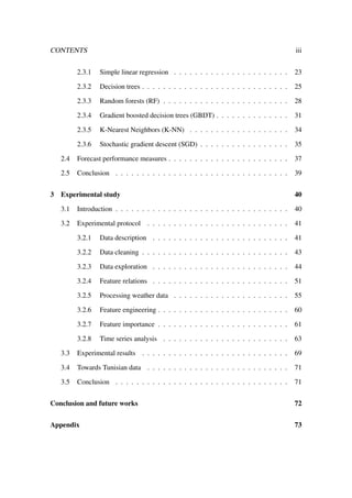
• q refers to moving average terms;
Example 1.2. Data was collected from an existing US airline. There is a sample of 5 city
pairs named A/B, B/A, D/C, E/F and F/E. A total of 28 flights (F1,F2,...,F28) were included
in the sample and final bookings for M class. Reservations data can be retrieved for the
boarding day (MBD), 7 (M7), 14 (M14), 21 (M21), 28 (M28) days before flight departure.
The sample period was from January, 1986 through June, 1986.
ARIMA(3,0,2) model were developed and estimated for flight F1 in the A/B market:
AR(3) × MBD(t) = C + MA(2) × r(t) (1.4)
where:
• AR(3) = ( 1 + AR(1) ×B + AR(2)×B2
+ AR(3) ×B3
;
• B = backward shift operator, defined as: Bn
[X(t)]= X(t-n);
• MBD(t) = final reservations, M-class at time t;
• MA(2) = ( 1 + MA(1) ×B + MA(2) × B2
);
• r(t)= residual at time t;
• C = constant;

Table 1.4 shows fitting results for an ARIMA(3,0,2) model. The model estimated is
statistically accepted, because the calculated chi-square test statistic on first 20 residual
autocorrelations is 17.9051, which is meaningful at least at a confidence level of 0.90, chi-
square(15,0.90) = 22.3. The estimated white noise variance is 77.56, which corresponds
to a standard error of regression of 8.81 8.89 (standard deviation of the time series
variable).
Table 1.4: Time Series Analysis ARIMA (3,0,2)
ITERATION 4: RESIDUAL SUM OF SQUARES .....13739
ITERATION 5: RESIDUAL SUM OF SQUARES .....13434.9
SUMMARY OF FITTED MODEL
parameter estimate stnd.error t-value prob(> |t|)
AR (1) 1.00765 0.14360 7.01705 0
AR (2) -0.11036 0.17264 -0.63922 0.52353
AR (3) 0.02083 0.08176 0.25474 0.79923
MA (1) 1.07407 0.14845 7.23533 0
MA (2) -0.22857 0.15545 -1.47036 0.14329
MEAN 22.04925 1.33373 16.53206 0
CONSTANT 1.87547
ESTIMATED WHITE NOISE VARIANCE = 77.5587 WITH 172
DEGREES OF FREEDOM.
CHI-SQUARE TEST STATISTIC ON FIRST 20 RESIDUAL
AUTOCORRELATIONS = 17.9051.
Example 1.3. The second model was estimated for the original series differenced once.
A week seasonality was introduced in the model ARIMA(0,1,4):
D(t) = C + MA(4) × r(t) (1.5)
where:
• D(t)= MBD(t) - MBD(t-1);
• MBD(t) = final reservations, M-class at time t;
• MA(4) = 1 + MA(7)×B7
+ MA(14)×B1
4 + MA(21)×B2
1 + MA(28)×B2
8;
• r(t) = residual at time t;
Table 1.5 shows fitting results for an ARIMA(0,1,4) model. The calculated chi-square
statistic is 17.7191 < 22.3, which means that the model can be accepted. Estimated white

noise variance, this time, was higher than before 108.23, which means a standard error of
regression of 10.40.
Table 1.5: Time Series Analysis ARIMA (0,1,4)
ITERATION 2: RESIDUAL SUM OF SQUARES .....15282
SUMMARY OF FITTED MODEL
parameter estimate stnd.error t-value prob(> |t|)
SAR (7) -0.70067 0.08339 -8.40285 0
SAR (14) -0.43076 0.10223 -4.21363 0.00004
SAR (21) -0.24550 0.10321 -2.37860 0.01872
SAR (28) -0.32319 0.09446 -3.42135 0.00082
MEAN -0.10325 0.30574 -0.33770 0.73609
CONSTANT -0.36782
MODEL FITTED TO SEASONAL DIFFERENCES OF ORDER 1
WITH SEASONAL LENGTH = 7.
ESTIMATED WHITE NOISE VARIANCE = 108.233 WITH 141
DEGREES OF FREEDOM.
CHI-SQUARE TEST STATISTIC ON FIRST 20 RESIDUAL
AUTOCORRELATIONS 17.7191.
These two examples illustrate the uncertainty of reservation data. Rather than showing
how to use ARIMA models, they serve to illustrate the difficulty for the forecaster in
modeling and the apparent limitation of time series models. Also, since no structural
behavior is associated with a time series model, the specification of the model becomes
extremely long. No clear approach to modeling can be developed, not in a reasonable way,
when using time series models. Too much intervention by the forecaster is required. Time
series analysis has been applied to the remaining markets and the results have been similar.
For these reasons, the use of time series analysis in forecasting reservations becomes
unattractive, although with only two model examples, a forecaster should never rule out
one forecasting method.
It should be noted that in the models presented above, only data related to reservations
on the day of boarding were used. No other available data, such as the reservation made
28 days before departure for the same flight, or the reservation for the same class on the
same day, or even other flight reservation data, was ever used. This leads to the next
Subsection which is the use of regression analysis in forecasting reservations.

1.4.2 Regression analysis
The use of regression analysis in forecasting bookings leads to the presumption that some-
thing is known about the cause-and-effect relationships that are relevant and that influence
booking patterns for a given flight. One can assume that there is a relationship between
reservation levels in a directional market, for example. Cause and effect relationships
can also be tested between different classes on the same flight/market. It could be argued
that some passengers who made a reservation on a full Y class did so because they could
not find a seat in ”compartment M”. The correlation between classes, between flights
and between markets are some examples that could be tested by developing a regression
model.
Example 1.4. The variables used in the general structure model to forecast bookings to
come, for flight F1 in M class, for a given market, from t days before departure, (Mt BD
), are as follows:
• ONE: a constant or base booking level;
• DAYS: day of week dummy variables, (MO,TU,WE,TH,FR, and SA relative to SU);
• Mt: bookings-on-hand, on day t, M-class;
• INDEX: week of year non-dimensionalized index for traffic levels and growth through
the major hub of the airline;
• S5MAt: historical average of bookings made in M-class, between day t and depar-
ture, for the most five recent departures of the same flight Fi;
• MTt: total bookings on hand, for all future flights in the same directional market t
days before departure.
Table 1.6 shows the results of the adjustment of the general structure model applied
to the A/B market, Flight F1. Ten explanatory variables are included in the model. The
model also includes a constant term. The model is fitted in a subset of the original data
set. The subset used ranged from observation #35 to observation #181, for a total of 147
observations. The sample size was reduced to 147 due to the S5MA variable. S5MA
is a 5-week lag average, and therefore the first non-trivial S5MA is for observation #35
(35=7.5).
The degree of freedom of the F statistic is therefore equal to 10 (the number of ex-
planatory variables) in the numerator, and equal to 136 (number of observations minus the
number of parameters to be estimated, i.e. 136=147-10-1) in the denominator. Therefore,

the critical value of the F-statistic (10,136), at the 95% confidence level, is 1.91. All series
have a higher F level, meaning that the models are accepted.
The adjusted R-squared, or R-squared bar, for all strokes is characterized by a low
value. Remember that the dependent variable is the result of the difference between final
bookings and current bookings. The model fit for differentiated variables will always have
a low value of R squared. This explains, to some extent, why the R-squared is relatively
low for each set of models.
Table 1.6: Regression analysis for flight F1 to market A/B
MODEL RUN (DAY) t=28 t=21 t=14 t=7
DEPENDENT VARIABLE M28 BD M21 BD Ml4 BD M7 BD
MEAN 15.56 14.44 12.01 7.56
STD. DEV. 8.32 8.24 7.72 6.09
STD. ERROR OF REGRESSION 6.38 6.34 6.09 5.35
R SQUARED 0.45 0.45 0.42 0.28
R-BAR SQUARED 0.41 0.41 0.38 0.23
F-STATISTIC (10,136) 11.17 l l.0l 9.79 5.29
VARIABLES value t stat value t stat value t stat value t stat
CONSTANT 34.56 6.57 33.87 6.46 31. 61 6.21 24.04 5.19
MO -3.94 -1.98 -3.86 -1.96 -2.85 -1.51 -1.36 -0.87
TU 0.41 0.19 0.45 0.21 1.34 0.66 2.14 1.21
WE 1.6 0.81 1.35 0.68 1.94 1.01 1.37 0.82
TH 3.12 1.34 3.31 1.42 3.39 1.52 2.28 1.18
FR 5.91 2.93 5.32 2.65 4.54 2.32 1.36 0.75
SA -5.l1 -2.52 -5.14 -2.55 -3.81 -1.94 -20.9 -1.21
Mt -0.51 -4.23 -0.49 -4.13 -0.42 -3.95 -0.29 -3.18
INDEX -0.11 -2.23 -0.09 -2.11 -0.11 -2.31 -0.08 -2.18
S5MAt -0.32 -2.15 -0.32 -2.16 -0.23 -1.62 -0.13 -1.04
MTt -0.15 -1.97 -0.15 -1.94 -0.16 -2.25 -0.09 -1.57
In this example, there was distinct behavior for Mondays, Fridays, Thursdays and
Saturdays. They were statistically different from the reference day, which was Sunday.
The Bookings-on-hand and INDEX variables were significant in all series: in each series,
the t-statistic of the coefficients was greater than the critical value t(136)=1.98. This
market/flight is an example of the model fitting results that is expected for the general
structure model. The variable INDEX should be significant and take into account the
seasonality of the week of the year. A ”local” seasonality should also be captured by
dummy variables of the day of the week. It was indeed possible for this flight/market to
detect a different behavior for some dummy variables.
On the whole, the results obtained via time series analysis (Box and Jenkins’ ARIMA
models) were not encouraging enough in providing better estimates, when compared to
results obtained via Regression analysis.

Section 1.5 – Conclusion 19
1.5 Conclusion
Understanding revenue and yield management concepts and their differences are essential
for any manager. Adopting an effective revenue or yield management system enables the
best pricing decisions and maximizes revenue with low margins.
This Chapter first presents the basics of revenue and yield management. Second, it
describes the important steps for RM and YM systems. Moreover, this Chapter defines
yield management forecasting methods using statistical analysis with a case study in the
airline industry.
In the next Chapter, YM forecasting methods will be presented using supervised Ma-
chine Learning algorithms for regression.

Chapter 2
Yield Management beyond Machine
Learning
2.1 Introduction
Machine Learning (ML) techniques plays a major role in accompanying predictive anal-
ysis due to its phenomenal performance in forecasting and also to manage large data
sets with uniform characteristics and noisy data. By applying machine learning models,
researchers are able to recognize the non-parametric patterns from data without setting
rigorous statistical assumptions. ML techniques are applicable in many sectors including
restaurant management.
ML techniques have many benefits for restaurants. They reduce food waste which
saves money and protects the environment. They allow past sales data to be reconciled
with weather conditions to calculate the amount of inventory needed to meet consumer
demand. They also have an impact on vacations and events. They mitigate losses by
using Artificial Intelligence (AI) techniques to forecast sales, inventory and staffing re-
quirements during seasonal vacations and major events. Our objective is to apply ML
techniques to restaurant revenue management problems in order to benefit from the power
of these techniques.
This Chapter is organized as follows: Section 2.2 states the problem of our work and
proposes a solution. Section 2.3 presents some supervised Machine Learning algorithms
for regression with illustrated examples of the data set. Finally, Section 2.4 defines the
major measures of efficiency for forecasting.
20

Section 2.2 – Problem statement 21
2.2 Problem statement
Given an historical data D (about reservations, visitors, locations, weather, etc), our goal is
to predict for any restaurants R = {r1, ..., rn} the number of visitors v in a time t. Formally,
the equation is presented as follows:
f(D, ri, t) = v (2.1)
where:
• f is the prediction function;
• D is the historical data;
• ri is a restaurant with index i;
• t is the time;
• v is the number of visitors;
This will help restaurant managers make informed decisions, better plan and allow
them to focus on creating an enjoyable dining experience for their visitors.
Figure 2.1 summarizes the whole situation.
Figure 2.1: Forecasting model for visitors
We follow a standard machine learning process which can be concluded as shown in
Figure 2.2.

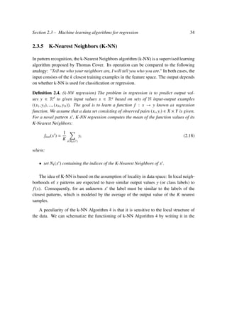
Section 2.3 – Machine learning algorithms for regression 22
Figure 2.2: Machine learning process chart for forecasting
The first steps were to understand the main problem, get familiar with the data struc-
ture and decide what features we need. In any modeling process, the data that goes into a
model plays an important role in ensuring accurate results.
2.3 Machine learning algorithms for regression
Artificial intelligence and machine learning have gained a strong foothold across different
industries due to their ability to streamline operations, save costs, and reduce human error.
ML has reshaped many sectors like healthcare, finance, retail, the restaurant industry, etc.
ML algorithms are often categorized as supervised or unsupervised.
• In a supervised learning model, the algorithm learns on a labeled data set, providing
an answer key that the algorithm can use to evaluate its accuracy on training data.
• An unsupervised model provides unlabeled data that the algorithm tries to make
sense of by extracting features and patterns on its own.

Figure 2.3: Schematic of machine learning
Regression algorithms fall under the family of supervised machine learning algorithms
which is a subset of machine learning algorithms. They predict the output values based
on input features from the data fed in the system. The go-to methodology is the algorithm
builds a model on the features of training data and using the model to predict the value
for new data.
2.3.1 Simple linear regression
Simple linear regression is a machine learning algorithm based on supervised learning
that models a linear relationship between a dependent variable y and a single independent
variable X.
Definition 2.1. (Simple linear regression) Formally, it can be defined as:
y ≈ β0 + β1X (2.2)
where:
• β0 and β1 are two unknown constants that represent the intercept and slope terms
(the model coefficients or parameters);
We will sometimes describe Equation 2.13 by saying that we are regressing y on X
(or y onto X).
Example 2.1. Table 2.1 describes an illustration of a data set which contains as variables
the number of visitors and the number of reservations per day for a period of one month
January, 2016.

Table 2.1: Illustration of a data set for simple linear regression algorithm
visit date reserve visitors count visitors
01/01/2016 100 80
02/01/2016 97 60
03/01/2016 80 70
04/01/2016 80 75
05/01/2016 85 67
06/01/2016 90 78
07/01/2016 95 88
08/01/2016 100 90
09/01/2016 120 100
Here, X may represent number of visitors’ reservations for a restaurant and y may
represent total number of visitors. Then we can regress Nbr visitors onto Nbr reservations
by fitting the model:
Nbr visitors ≈ β0 + β1 × Nbr reservations (2.3)
Once we have used our coefficient parameter training data to produce estimates ˆβ0 and ˆβ1
for the model coefficients, we can predict future Nbr of visitors on the basis of a particular
value of Nbr of reservations by computing:
ˆy = ˆβ0 + ˆβ1X (2.4)
where:
• ˆy indicates a prediction of y on the basis of X = x.
Figure 2.4 shows a real Nbr of visitors in these red points and the regression line contain-
ing the predicted Nbr of visitors. We can see for example in Figure (a), the predicted Nbr
of visitors corresponding to 250 Nbr of reservations is about 225 Nbr of visitors per day.
Our predicted visitors are very close to the real visitors for most of them on both training
and test set.

(a) train set
(b) test set
Figure 2.4: Visitors vs reservations with simple linear regression algorithm
2.3.2 Decision trees
Decision trees are a type of supervised learning algorithm for predictive modelling and
can be used to visually and explicitly represent decisions.
Regression trees are used to predict a quantitative response (e.g. the age, the number

of visitors). The predicted response for an observation is given by the mean response of
the training observations that belong to the same terminal node.
Definition 2.2. The data consists of p inputs and a response, for each of N observa-
tions: that is, (xi, yi) for i = 1, 2, ..., N, with xi = (xi1, xi2, ..., xip). The algorithm needs
to automatically decide on the splitting variables and split points, and also what topol-
ogy (shape) the tree should have. Suppose first that there is a partition into M regions
R1, R2, ..., RM, and the response model will be like a constant cm in each region:
f(x) =
M
m=1
cmI(x ∈ Rm) (2.5)
If the minimization criterion will be adopted of the sum of squares (yi − f(xi))2
, it’s easy
to see that the best ˆcm is just the average of yi in region Rm:
ˆcm = avg(yi | xi ∈ Rm) (2.6)
Finding the best binary partition in terms of minimum sum of squares is usually not com-
putationally feasible, so the greedy algorithm will proceed. Starting with all data, a divi-
sion variable j and a division point s will be considered, and the pair of half-planes will
be defined.
R1(j, s) = {X | Xj s} and R2(j, s) = {X | Xj > s} (2.7)
Next, look for the splitting variable j and split point s that solve:
min
j,s
[ min
c1
xi∈R1(j,s)
(yi − c1)2
+ min
c2
xi∈R2(j,s)
(yi − c2)2
] (2.8)
For any choice j and s, the inner minimization is solved by
ˆc1 = avg (yi | xi ∈ R1(j, s)) and ˆc2 = avg (yi | xi ∈ R2(j, s)) (2.9)
For each splitting variable, the determination of the split point s can be performed very
quickly and, therefore, by scanning all inputs, the determination of the best pair (j, s) is
possible. Once the best split has been found, the data must be divided into two resulting
regions and the process of dividing on each of the two regions must be repeated. Then
this process is repeated on all resulting regions.
Tree size is a tuning parameter governing the model’s complexity, and the optimal
tree size should be adaptively chosen from the data. One approach would be to split tree
nodes only if the decrease in sum-of-squares due to the split exceeds some threshold. This

strategy is too short-sighted, however, since a seemingly worthless split might lead to a
very good split below it.
The preferred strategy is to grow a large tree T0, stopping the splitting process only
when some minimum node size (say 5) is reached. Then this large tree is pruned using
cost-complexity pruning.
Suppose a sub-tree T ⊂ T0 to be any tree that can be obtained by pruning T0, that
is, collapsing any number of its internal (non-terminal) nodes. The terminal nodes are
indexed by m, with node m representing region Rm. Let |T| denote the number of terminal
nodes in T.
Nm = # {xi ∈ Rm};
ˆcm =
1
Nm xi∈Rm
yi;
Qm(T) =
1
Nm xi∈Rm
(yi − ˆcm)2
;
(2.10)
The cost complexity criterion is:
Cα(T) =
|T|
m=1
NmQm(T) + α|T| (2.11)
The idea is to find, for each α, the sub-tree Tα ⊆ T0 to minimize Cα(T). The tuning
parameter α 0 governs the trade-off between tree size and its goodness of fit to the data.
Large values of α result in smaller trees Tα, and conversely for smaller values of α. As the
notation suggests, with α = 0 the solution is the full tree T0. How to adaptively choose
α? For each α one can show that there is a unique smallest sub-tree Tα that minimizes
Cα(T). To find Tα, use weak link pruning: successively collapse the internal node that
produces the smallest increase per node of m NmQm(T), and continue until producing
the single node (root) tree. This gives a (finite) sequence of sub-trees, and one can show
this sequence must contain Tα.
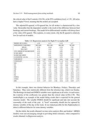
Example 2.2. , Figure 2.5 explains the popular method for tree-based regression called
CART with our data base. we took as independent variables X all the attributes of the
database except the number of visitors. For the dependent variable y we took the number
of visitors. A detailed description of the database will be presented in Subsection 3.2.1.
We can say that:
If X[6] ≤ 0.645 and X[6] ≤ 1.562 and X[6] ≤ 2.545 then predict 1.628.
If X[6] ≤ 0.645 and X[6] ≤ 1.562 and X[6] ≤ 1.16 then predict 0.646.
If X[6] ≤ 0.645 and X[6] ≤ −0.438 and X[6] ≤ −1.752 then predict -0.588.
If X[6] ≤ 0.645 and X[6] ≤ −0.438 and X[6] ≤ 0.212 then predict 0.01.

Figure 2.5: Application of regression tree with the CART method
Algorithm 1: Building a regression tree
1 Use recursive binary splitting to grow a large tree on the training data, stopping
only when each terminal node has fewer than some minimum number of
observations;
2 Apply cost complexity pruning to the large tree in order to obtain a sequence of
best sub-trees, as a function of α;
3 Use K-fold cross-validation to choose α. That is, divide the training observations
into K folds. For each k = 1, ..., K;
4 Repeat Steps 1 and 2 on all but the kth fold of the training data;
5 Evaluate the mean squared prediction error on the data in the left-out kth fold,
as a function of α;
6 Average the results for each value of α, and pick α to minimize the average
error;
7 Return the sub-tree from Step 2 that corresponds to the chosen value of α;
2.3.3 Random forests (RF)
Random forests are a decision trees based method and they were introduced by (Breiman,
2001), who was inspired by earlier work by (Amit and Geman, 1997). They are an exten-
sion of Breiman’s bagging or bootstrap aggregation, which is a technique for reducing the
variance of an estimated prediction function. Also, they were developed as a competitor
to boosting, which is appeared to dominate bagging on most problems, and became the

preferred choice. RF can be used for either classiﬁcation and regression.
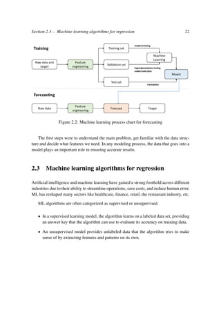
Example 2.3. For random forests, we will work on the same example of the data set
explained in Subsection 2.3.2. We train a random forest with 10 estimators, and maximal
depth = 3 on our data set. The random forest model is then an ensemble model of 10
regression tree estimators, each of them has a maximal depth equal to 3 (See Figure 2.6).
Note that variable X[6] corresponding to annual average visitors is present on several
nodes in all the trees of the trained random forest. It suggest that this feature is the most
informative. This observation is also conﬁrmed by Figure 3.21 (See Subsection 3.2.7 for
more details about feature importance).

Figure 2.6: Individual estimators (trees) learnt by random forest applied on our data set.
Each estimator is a binary regression tree with maximal depth = 3.

Algorithm 2: Random forests for regression algorithm
Input :
Output: ˆf B
r f (x) = 1
B
B
b=1 Tb(x);
1 for b = 1 to B: do
2 Draw a bootstrap sample Z∗
of size N from the training data;
3 Grow a random-forest tree Tb to the bootstrapped data, by recursively
repeating the following steps for each terminal node of the tree, until the
minimum node size nmin is reached;
4 Select m variables at random from the p variables;
5 Pick the best variable/split-point among the m;
6 Split the node into two daughter nodes;
7 end
2.3.4 Gradient boosted decision trees (GBDT)
In 1999, Jerome Friedman introduced Gradient Boosted Decision Trees (GBDT) algo-
rithm which is another type of supervised learning algorithm for predictive modelling.
GBDT is a widely-used machine learning algorithm, due to its efficiency, accuracy, and
interpretability.
Definition 2.3. (Gradient boosted decision trees) Assuming that x is a set of predictor
variables and f(x) is an approximation function of the response variable y, using the
training data {xi, yi}N
1 , the GBDT approach iteratively constructs M different individual
decisions trees h(x, a1), ..., h(x, aM), then f(x) could be expressed as an additive expansion
of basis function h(x, am) as follows:
f(x) = M
m=1 fm(x) = M
m=1 βmh(x, am)
h(x, am) = J
j=1 γjmI(x ∈ R), where I = 1 if x ∈ Rjm; I = 0, otherwise.
(2.12)
where:
• Each tree partitions the input space into J disjoint regions R1m, ..., Rjm and predicts
a constant value γjm for region Rjm;
• βm represents weights given to the nodes of each tree in the collection and determine
how predictions from the individual decision trees are combined (De’Ath, 2007);
• am represents the mean values of split locations and the terminal node for each
splitting variables in the individual decision tree;
The parameters βm and am are estimated by minimizing a specified loss function L(y, f(x))
that indicates a measure of prediction performance (Saha et al., 2015).

Defining an additive function that is combined from the first decision tree to the (m1)th
decision tree as fm1(x), the parameters βm and am should be determined as follows (Fried-
man, 2002):
(βm, am) = arg min
β,a
N
i=1
L(yi, fm−1(xi) + βh(xi, a))
= arg min
β,a
N
i=1
L(yi, fm−1(xi) + β
J
j=1
γjI(xi ∈ Rj))
(2.13)
and
fm(x) = fm−1(x) + βmh(x, am) = fm−1(x) + βm
J
j=1
γjmI(x ∈ Rjm) (2.14)
Generally, it is not straightforward to solve Equation (2.13) due to the poor performance
of squared error loss and exponential loss functions for non-robust data or censored data
(Friedman et al., 2001). To overcome this problem, Friedman devised the gradient boost-
ing approach (Friedman et al., 2001), which is an approximation technique that applies
the method of steepest descent to forward stagewise estimation. Gradient boosting ap-
proximation can solve the above equation for arbitrary loss functions with a two-step
procedure. First, the parameters am for the decision tree can be estimated by approximat-
ing a gradient with respect to the current function fm−1(x) in the sense of least square error
as follows:
am = arg min
a,β
N
i=1
˜yim − βh(xi, a) 2
= arg min
a,β
N
i=1

˜yim − β
J
j=1
γjI(xi ∈ Rj)


2
(2.15)
where ˜yim is the gradient and is given by
˜yim = −
∂L(yi, f(xi))
∂f(xi) f(x)=fm−1(x)
(2.16)
Then, the optimal value of the parameters βm can be determined given h(x, am):
βm = arg min
β
N
i=1
L(yi, fm−1(xi) + βh(xi, am))
= arg min
β
N
i=1
L(yi, fm−1(xi) + β
J
j=1
γjmI(xi ∈ Rjm))
(2.17)
The gradient boosting approach replaces a potentially difficult function optimization prob-
lem in Equation (2.13) with the least-squares function minimization as Equation (2.15),

and then, the calculated am can be introduced into Equation (2.17) for a single parameter
optimization. Thus, for any h(x, a) for which a feasible least-squares algorithm exists,
optimal solutions can be computed by solving Equations (2.15) and (2.17) via any dif-
ferentiable loss function in conjunction with forward stagewise additive modeling. Based
on the above discussion, the algorithm for the gradient boosting decision trees can be
summarized in Algorithm 3 (Friedman et al., 2001).
Algorithm 3: Gradient boosted decision trees for regression algorithm
Input: Data {xi, yi}N
i=1, and a diﬀerentiable Loss Function L(yi, f(x));
Result: f(x) = M
m=1 fm(x);
1 Initialize f0(x) to be a constant, f0(x) = arg minβ
N
i=1 L(yi, β);
2 for m=1 to M do
3 for i=1 to N do
4
˜yim = −
∂L(yi, f(xi))
∂ f(xi) f= fm−1
5 end
6 Fit a regression tree h(x, am) to the targets ˜yim giving terminal regions
Rjm, j = 1, 2, ..., Jm;
7 Compute a gradient descent step size as
βm = arg min
β
N
i=1
L(yi, fm−1(xi) + βh(xi, am))
Update the model as fm(x) = fm−1(x) + βmh(x, am);
8 end
Example 2.4. Figure 2.7 is a presentation of the decision tree learnt by XGB Regressor
(GBDT) when trained on our data set.
Figure 2.7: The regression tree found by XGB Regressor (GBDT)

2.3.5 K-Nearest Neighbors (K-NN)
In pattern recognition, the k-Nearest Neighbors algorithm (k-NN) is a supervised learning
algorithm proposed by Thomas Cover. Its operation can be compared to the following
analogy: ”Tell me who your neighbors are, I will tell you who you are.” In both cases, the
input consists of the k closest training examples in the feature space. The output depends
on whether k-NN is used for classiﬁcation or regression.
Deﬁnition 2.4. (k-NN regression) The problem in regression is to predict output val-
ues y ∈ Rd
to given input values x ∈ Rq
based on sets of N input-output examples
((x1, y1), ..., (xN, yN)). The goal is to learn a function f : x → y known as regression
function. We assume that a data set consisting of observed pairs (xi, yi) ∈ X × Y is given.
For a novel pattern x , K-NN regression computes the mean of the function values of its
K-Nearest Neighbors:
fknn(x ) =
1
K i∈Nk(x )
yi (2.18)
where:
• set Nk(x ) containing the indices of the K-Nearest Neighbors of x .
The idea of K-NN is based on the assumption of locality in data space: In local neigh-
borhoods of x patterns are expected to have similar output values y (or class labels) to
f(x). Consequently, for an unknown x the label must be similar to the labels of the
closest patterns, which is modeled by the average of the output value of the K nearest
samples.
A peculiarity of the k-NN Algorithm 4 is that it is sensitive to the local structure of
the data. We can schematize the functioning of k-NN Algorithm 4 by writing it in the

following pseudo-code.
Algorithm 4: K-Nearest Neighbors regression (KNNR) algorithm
Input: A n × n distance matrix D[1...n, 1...n] and an index s of the starting city.
Result: A list Path of the vertices containing the tour is obtained
1 for i ← 1 to n do
2 Visited [i] ← false;
3 end
4 Initialize the list Path with s;
5 Visited[s] ← true;
6 Current ← s;
7 for i ← 2 to n do
8 Find the lowest element in row current and unmarked column j containing
the element;
9 Current ← j;
10 Visited[j] ← true;
11 Add j to the end of list Path;
12 end
13 Add s to the end of list Path;
14 return Path
2.3.6 Stochastic gradient descent (SGD)
Deﬁnition 2.5. (Stochastic gradient descent) Let us ﬁrst consider a simple supervised
learning setup. Each example z is a pair (x, y) composed of an arbitrary input x and a
scalar output y. We consider a loss function (ˆy, y) that measures the cost of predicting ˆy
when the actual answer is y, and we choose a family F of functions fw(x) parameterized by
a weight vector w. We seek the function f ∈ F that minimizes the loss Q(z, w) = (fw(x), y)
averaged on the examples. Although we would like to average over the unknown distri-
bution dP(z) that embodies the Laws of Nature, we must often settle for computing the
average on a sample z1...zn.
E(f) = (f(x), y) dP(z)
En(f) =
1
n
n
i=1
( f(xi), yi)
(2.19)
where:
• The empirical risk En(f) measures the training set performance.

• The expected risk E(f) measures the generalization performance, that is, the ex-
pected performance on future examples.
The statistical learning theory (Vapnik and Chervonenkis, 2015) justifies minimizing
the empirical risk instead of the expected risk when the chosen family F is sufficiently
restrictive.
Gradient descent (GD)
It has often been proposed (Rumelhart et al., 1985) to minimize the empirical risk En(fw)
using gradient descent (GD). Each iteration updates the weights w on the basis of the
gradient of En(fw):
wt+1 = wt − γ
1
n
n
i=1
wQ(zi, wt) (2.20)
where:
• γ is an adequately chosen learning rate.
Under sufficient regularity assumptions, when the initial estimate w0 is close enough to
the optimum, and when the learning rate γ is sufficiently small, this algorithm achieves
linear convergence (Dennis Jr and Schnabel, 1996), that is, −log p ≈ t, where p represents
the residual error. Much better optimization algorithms can be designed by replacing the
scalar learning rate γ by a positive definite matrix Γt that approaches the inverse of the
Hessian of the cost at the optimum:
wt+1 = wt − Γt
1
n
n
i=1
wQ(zi, wt) (2.21)
This second order gradient descent (2GD) is a variant of the well known Newton al-
gorithm. Under sufficiently optimistic regularity assumptions, and provided that w0 is
sufficiently close to the optimum, second order gradient descent achieves quadratic con-
vergence. When the cost is quadratic and the scaling matrix Γ is exact, the algorithm
reaches the optimum after a single iteration. Otherwise, assuming sufficient smoothness,
we have−log log p ≈ t.

Section 2.4 – Forecast performance measures 37
Stochastic gradient descent (SGD)
The stochastic gradient descent (SGD) algorithm is a drastic simplification. Instead of
computing the gradient of En(fw) exactly, each iteration estimates this gradient on the
basis of a single randomly picked example zt:
wt+1 = wt − γt wQ(zt, wt) (2.22)
The stochastic process {wt, t = 1, ..., n} depends on the examples randomly picked at each
iteration. It is hoped that Equation (2.22) behaves like its expectation Equation (2.20)
despite the noise introduced by this simplified procedure.
Since the stochastic algorithm does not need to remember which examples were vis-
ited during the previous iterations, it can process examples on the fly in a deployed system.
In such a situation, the stochastic gradient descent directly optimizes the expected risk,
since the examples are randomly drawn from the ground truth distribution.
2.4 Forecast performance measures
Since there are a various number of forecasting methods, it is essential to have objective
criteria by which to evaluate these methods, which are specified structure, plausible struc-
ture, acceptability, explanatory power, robustness, parsimony, cost and accuracy. (Witt
et al., 1992) found out that the accuracy is the most important forecast evaluation crite-
rion. Through precision measurements of the magnitude of errors, we can evaluate the
accuracy of certain forecasting methods.
In each of the forthcoming forecasting methods:
• yt is the actual value;
• ft is the forecasted value;
• et = yt − ft is the forecast error;
• n is the size of the test set;
• ¯y = 1
n
n
t=1 yt is the test mean;
• σ2
= 1
n−1
n
t=1(yt − ¯y)2
is the test variance;

Section 2.4 – Forecast performance measures 38
Definition 2.6. (Mean Absolute Error (MAE)) The Mean Absolute Error (MAE) is defined
as (Hamza¸cebi, 2008):
MAE =
1
n
n
t=1
|et| (2.23)
Definition 2.7. (Mean Absolute Percentage Error (MAPE)) The Mean Absolute Percent-
age Error (MAPE) is given by (Hamza¸cebi, 2008):
MAPE =
1
n
n
t=1
|
et
yt
| × 100 (2.24)
Definition 2.8. (Mean Squared Error (MSE)) The Mean Squared Error (MSE) is given by
(Hamza¸cebi, 2008; Zhang, 2003):
MS E =
1
n
n
t=1
e2
t (2.25)
Definition 2.9. (Root Mean Squared Logarithmic Error (RMSLE)) The Root Mean Squared
Logarithmic Error (RMSLE) is given by (Gandomi and Haider, 2015):
RMS LE =
1
n
n
i=1
(ln(pi + 1) − ln(ai + 1))2 (2.26)
where:
• n is the number of predictions in the test set;
• pi the number i prediction value;
• ai the number i actual value of visitors;
Definition 2.10. (R-squared (R2
)) The R-squared (Coefficient of determination) repre-
sents the coefficient of how well the values fit compared to the original values. The value
from 0 to 1 interpreted as percentages. The higher the value is, the better the model is.
R2
= 1 −
(yi − ˆy)2
(yi − ¯y)2
(2.27)
where:
• ˆy is the predicted value of y;
• ¯y is the mean value of y;

Section 2.5 – Conclusion 39
2.5 Conclusion
Machine learning has many applications in restaurants, including predicting the number
of future visitors at earlier dates to optimize revenue. As a result, it can help restau-
rants operate more eﬃciently, reduce food waste and allow restaurateurs to focus on areas
where they can add the most value. This Chapter proposes a new solution to predict
the number of visitors for restaurants in future dates and presents Machine Learning re-
gression algorithms. The results of these supervised algorithms will be compared using
forecast performance measures.
In order to evaluate our proposed solution, we provide in the next Chapter an experi-
mental study performed to a real-world data set.

Chapter 3
Experimental study
3.1 Introduction
Running a successful local restaurant is not always an easy task as first impressions sug-
gest. Often, all kinds of unexpected problems arise that can be detrimental to business.
One of the most common challenges is that restaurant managers need to know how many
visitors to expect each day to efficiently purchase ingredients and schedule staff members.
This forecasting is not easy to do because there are many unpredictable factors that af-
fect restaurant attendance, such as weather, a nation’s uncontrollable economic cycles or
natural disasters.
In this last Chapter, we did the data pre-processing (cleaning and organization) which
is a crucial step to improve data quality in order to promote the extraction of useful infor-
mation from the data and make it suitable for a building and training Machine Learning
models. We have also done graphical analyses of the data that will help us present the
data in a meaningful way to make good decisions. Finally, we tested and compared our
model with different statistical methods and machine learning to better predict the future
number of visitors for restaurants.
This Chapter is organized as follows: Section 3.2 presents the experimental proto-
col. Section 3.3 discusses the different results found by statistical and machine learning
methods.
40

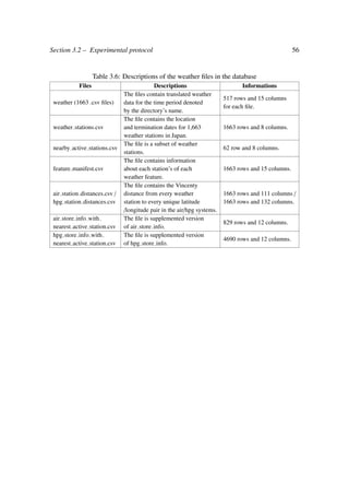
Section 3.2 – Experimental protocol 41
3.2 Experimental protocol
3.2.1 Data description
Data are taken from Kaggle1
competition and they are presented in the shape of 8 re-
lational ﬁles which are derived from two separate Japanese websites that collect user
information:
• Hot Pepper Gourmet (HPG): similar to Yelp, here users can search restaurants and
also make a reservation online.
• AirREGI / Restaurant Board (Air): similar to Square, a reservation control and cash
register system.
The database contains two main parts, the training data set and the test data set. We saw
from all the training data that:
• Total number of unique AIR restaurants is 829.
• Total number of current restaurants in AIR and HPG is 150.
• Total unique genre in AIR restaurants is 14.
• Total number of AIR restaurant’s locations is 103.
• Training data duration is from the 1st January 2016 to the 22th of April 2017.
Also, we saw from all the test data that:
• Total unique restaurants is 821.
• Test data duration is from the 23th April 2017 to the 31st of May 2017.
Table 3.1 represents the individual ﬁles and Table 3.2 details the attributes of the
database.
1
https://www.kaggle.com/c/recruit-restaurant-visitor-forecasting

Table 3.1: Descriptions of the database files
Files Descriptions Informations
air store info.csv /
hpg store info.csv
The files contain informations
about the air / hpg restaurants.
829 rows and 5 columns /
4690 rows and 5 columns
air reserve.csv /
hpg reserve.csv
The files contain reservations made
through the air / hpg systems.
store id relation.csv
This file allows you to join select
restaurants that have both
the air and hpg system.
air visit data.csv
The file contains historical visit
data for the air restaurants.
sample submission.csv
This file shows a submission in the
correct format, including the days
for which you must forecast.
date info.csv
This file gives basic information about
the calendar dates in the data set.
Table 3.2: Descriptions of the database attributes
Attributes Descriptions
Air store id The restaurant’s id in the air system.
Hpg store id The restaurant’s id in the hpg system.
Visit datetime The time of the reservation.
Reserve datetime The time the reservation was made.
Reserve visitors The number of visitors for that reservation.
Air genre name The genre of food for the restaurant in air system.
Air area name The name of the restaurant area in air system.
Latitude The latitude of the restaurant area.
Longitude The longitude of the restaurant area.
Hpg genre name The genre of food for the restaurant in hpg system.
Hpg area name The name of the restaurant area in hpg system.
Visit date The date.
Visitors The number of visitors to the restaurant on the date.
Holiday flg The day a holiday in Japan.
Day of week The day of the week.
Table 3.3 and Table 3.4 describe two illustrations of the data set.

Table 3.3: Sample from air reserve data set
air store id visit datetime reserve datetime reserve visitors
air 789466e488705c93 02/01/2016 17:00 02/01/2016 17:00 41
air 789466e488705c93 02/01/2016 17:00 02/01/2016 17:00 13
air 2b8b29ddfd35018e 02/01/2016 18:00 02/01/2016 17:00 2
air 6b15edd1b4fbb96a 02/01/2016 18:00 01/01/2016 12:00 3
air 877f79706adbfb06 02/01/2016 18:00 01/01/2016 16:00 2
Table 3.4: Sample from air store info data set
air store id air genre name air area name latitude longitude
air fa12b40b02fecfd8 Italian/French
TÅkyÅ-to Meguro
-ku Takaban
35.629 139.684
air fdc02ec4a3d21ea4 Dining bar
HyÅgo-ken KÅbe
-shi KumoidÅri
34.695 135.197
air c77ee2b7d36da265 Cafe/Sweets
Fukuoka-ken Fukuoka
-shi DaimyÅ
33.589 130.392
air 1d1e8860ae04f8e9 Izakaya
TÅkyÅ-to Shinjuku
-ku KabukichÅ
35.693 139.703
air df843e6b22e8d540 Bar/Cocktail
TÅkyÅ-to Minato
-ku ShibakÅen
35.658 139.751
3.2.2 Data cleaning
In real world data, there are some instances where a particular element is absent because
of various reasons, such as, corrupt data, failure to load the information, or incomplete
extraction. Handling the missing values is one of the greatest challenges faced by analysts,
because making the right decision on how to handle it generates robust data models.

Table 3.5: Missing values analysis
Function Display Function Display
air visit data.isnull().sum()
air store id = 0
visit date = 0
visitors = 0
dtype: int64
date info.isnull().sum()
calendar date = 0
day of week = 0
holiday ﬂg = 0
dtype: int64
air store info.isnull().sum()
air store id = 0
air genre name = 0
air area name = 0
latitude = 0
longitude = 0
dtype: int64
hpg store info.isnull().sum()
hpg store id = 0
hpg genre name = 0
hpg area name = 0
latitude = 0
longitude = 0
dtype: int64
air reserve.isnull().sum()
air store id = 0
visit datetime = 0
reserve datetime = 0
reserve visitors = 0
dtype: int64
hpg reserve.isnull().sum()
hpg store id = 0
visit datetime = 0
reserve datetime = 0
reserve visitors = 0
dtype: int64
store id relation.isnull().sum()
air store id = 0
hpg store id = 0
dtype: int64
sample submission.isnull().sum()
id = 0
visitors = 0
dtype: int64
Table 3.5 shows that there are no null values in the data set. So, there is no need of
performing any kind of missing data imputation.
3.2.3 Data exploration
Data exploration refers to the initial step in data analysis in which data analysts use data
visualization and statistical techniques to describe data set characterizations in order to
better understand the nature of the data. We examined the distributions of the feature in
our data set before combining them for a more detailed analysis. This initial visualization
will be the basis on which we will build our analysis.

Visitors analysis
Figure 3.1 presents the Probability Density Function (PDF) of average visitors per restau-
rant is almost normal(approx) with mean visitors 20.97, with a slight right skewness and
there are a large number of restaurants which have a capacity of less than 20. Further-
more, Friday and the weekend appear to be the most popular days, which is to be expected.
Monday and Tuesday have the lowest numbers of average visitors. Also during the year
there is a certain amount of variation. December appears to be the most popular month
for restaurant visits. The period from March to May is consistently busy.
Figure 3.1: PDF of average visitors per restaurant
Figure 3.2 shows that the minimum number of visitors is almost reaching zero, the
mean of the visitors is 20 (approx) and the maximum number of visitors is between 55-60.
We observed certain very high values (outlier) greater than 60 and and even greater than
100 visitors. 25th percentile and 75th percentile values are 13 (approx) and 30 (approx)
respectively.

Figure 3.2: Boxplot of average visitors per restaurant
Next, we can saw from Figure 3.3 Saturday is the day when most people prefer to go
out to eat, having the largest number of visitors throughout the year, the reason being that
it is the weekend. After Saturday, even on Sunday, there is a peak of visitors. On Monday,
the number of people going out to eat is the lowest. The other days of the week have an
almost similar trend in terms of the number of visitors. The sharp decline after the 51st
week is due to New Year’s Eve because most of the restaurants remain closed.
Figure 3.3: Visitors by day of the week

Figure 3.4 shows even on a daily basis, the restaurants see the most visitors on Satur-
days. Sunday is the second busiest period. Monday and Tuesday have the lowest number
of visitors. Thursday and Wednesday have almost the same attendance patterns.
Figure 3.4: Average visitors each day of week
We have observed by Figure 3.5 the average number of visitors is very high in the
month of December because it’s a month’s vacation. After December, March is the busiest
month. August and November is the month with the lowest number of visitors.
Figure 3.5: Average visitors each month

Reservations analysis
Now, we will see how our reservations data compares to the actual visitor numbers.
Figure 3.6: PDF of average visitors reservations per restaurant
Figure 3.6 shows that the spread of AIR reservations is higher than that of HPG reser-
vations. Also, there is a large number of reservations in HPG with visitors count between
5 to 10 and few reservations in HPG where the visitors count is more than 20 or even
reaching 40. Even in AIR, the maximum number of visitors registered is 40, but the num-
ber of registrations are more than that of HPG. Furthermore, the maximum number of
registrations in AIR have visitors count between 8 to 13 (approx).
Figure 3.7: Boxplot of average visitors reservations per restaurant

Figure 3.7 shows that the average number of reservations is less than 10. In AIR,
the average number of reservations is 10(approx) and in HPG, the average number of
reservations is 6(approx). 25th and 75th percentile number of reservations in AIR is 7
and 15 respectively. However, 25th and 75th percentile number of reservations in HPG is
4 and 8 respectively. In AIR, there are certain high values (outliers) we saw in the range
40 to 100 but in HPG, we saw certain high values (outliers) in the range 13 to 40.
Genre wise restaurant market share
After viewing the number of visitors per restaurant, the number of reservations per restau-
rant and the temporal aspects, we looked at the spatial information. Figure 3.8 shows that
restaurants in Japan are subdivided into 14 types of food. Izakaya is the most popular
genre in Japan as almost 23.8% of restaurants are of Izakaya genre. The second most
popular genre in Japan is Cafe/Sweets having almost 21.8% restaurant market share. In-
ternational cuisine, Asian and Karaoke/Party are the least preferred genre having only
0.2% each market share. Even western and korian food are not popular in japan at all.
Figure 3.8: Genre wise restaurant market share
To start a restaurant business in Japan, choosing food genre will be the most important
decision.

Date information
In this part, we focused on the holidays. We’re going to determine how many there are in
total and how they’re distributed over our forecast period in 2017 and the corresponding
period in 2016.
Figure 3.9: Description of the date info ﬁle
Figure 3.9 shows that the same days are public holidays in late April and early May
in both 2016 and 2017.
Train and test data sets
The training data is based on the period January 2016 to April 2017, while the test set
includes the last week of April plus May 2017.
The test data intentionally covers one week of vacation (Golden Week). The descrip-
tion of the data further indicates that there are days in the test set when the restaurant was
closed and had no visitors. These days are ignored in the scoring. The training set omits
the days when the restaurants were closed. Figure 3.10 shows the time interval between
the train and the test data sets.

Figure 3.10: Plot of train and test data sets
3.2.4 Feature relations
Visitors and reservations
According to the Figure 3.11, the increase in mid 2016 is due to the addition of new restau-
rants to the database. We found that the number of unregistered visitors is much higher
than the number of registered visitors. In addition, we have noticed a sharp decrease on
New Year’s Eve, as most restaurants remain closed on New Year’s Eve. Moreover, the
number of registered visitors in AIR is higher than the number of registered visitors in
HPG. The maximum number of visitors is observed in the month of December. As we
know, there are a number of festivities in December.
Figure 3.11: Relation between visitors and reservations

Hourly visitors behaviour
Figure 3.12 shows that the number of registrations in AIR is more than HPG. There is a
small hike after 10:00 AM, as that is the time when people go to oﬃce. The evening time
is quite busy. The highest number of visitors is between 5:30 PM to 7:00 PM (approx).
After 7:00 PM., the number of visitors declines sharply. There are no visitors between
12:00 AM and 7:00 AM (approx), it may be because restaurants stay closed during night.
Figure 3.12: Hourly visitors behaviour
We are also interested in the analysis of the time (shown here in hours) between the
reservation and the restaurant visit, which follows a 24 Hours pattern as shown in Figure
3.13. Most customers make reservations on the same day of the visit and then the time
curve starts to gradually decrease.
Figure 3.13: Analysis of the time between the reservation and the visit to the restaurant

Visitors vs genre
Figure 3.14 shows there are around 14 genres of food served by Japanese restaurants.
The most popular and the most liked genre is Izakaya followed by Cafe/Sweets which are
liked by maximum number of people.
Figure 3.14: Total visitors by air genre name
Asian, Karaoke/Party and International Cuisine are the emerging genre in Japan with
least customers. Even the Western Food is not liked much in Japan. The food genre is the
most important factor for growth in Japanese restaurant business.
Reservations vs genre
Figure 3.15 shows that Izakaya is the most popular genre for reservation trends. In the
unregistered visitors trends, we observed that Cafe/Sweets are the second most popular
genre, but here Italian/French is the second most popular genre. Aisan and International
Cuisine are the least popular as we have seen in previous plot. Surprisingly, the Japanese
Food is the 4th popular genre in Japan.

Figure 3.15: Reserve visitors by genre
The impact of holidays on visitors
In this Subsection, we will study the inﬂuence of holidays on the number of visitors by
comparing the statistics of days with holidays and days without holiday ﬂags.
Figure 3.16: Average visitors on holidays and non-holidays

It is evident from Figure 3.16 that it is obvious to have more visitors on holidays
than on working days. Also, the difference between visitors on holidays and those on
working days is not very significant, which is due to the weekend effect. For this reason,
when processing the data, we have to take into account the public holidays that come on
weekends, these public holidays should only be considered as weekends and not as public
holidays, just to take into account the weekend effect.
3.2.5 Processing weather data
Improving the accuracy of basic weather forecasts is also important for restaurants, as
these forecasts inform operational decisions and inaccurate forecasts can be detrimental
to visitor experience and demand. With Machine Learning, restaurants can accurately
forecast their sales based on the day of the week, previous sales results and weather con-
ditions. For instance, if a restaurant sold a large volume of alcoholic beverages on rainy
days last year, the machine learning-based forecasting solutions will cross-reference all
of these data points and indicate which menu items generate the most sales for that time
of year and weather conditions.
Data description
In this master thesis, we used detailed meteorological data from the official website of
the Japan Meteorological Agency, which were extracted and provided as a data set. This
data set is characterized by a period ranging from the 1st January 2016 to the 31st of May
2017 and contained 1663 files (one for each of the 1663 stations in Japan). The focus is
on using reservation data from various restaurants in Japan, as well as the location and
type of restaurants, to predict the actual number of visitors a restaurant will have on a
given day. This data set augments the above with the addition of information about the
weather at various locations in Japan over time to produce an exciting, multi-faceted data
set that deals with time, geography, weather, and food. Table 3.6 represents the files and
Table 3.7 details the attributes of the weather database.

Table 3.6: Descriptions of the weather files in the database
Files Descriptions Informations
weather (1663 .csv files)
The files contain translated weather
data for the time period denoted
by the directory’s name.
for each file.
weather stations.csv
The file contains the location
and termination dates for 1,663
weather stations in Japan.
1663 rows and 8 columns.
nearby active stations.csv
The file is a subset of weather
stations.
62 row and 8 columns.
feature manifest.csv
The file contains information
about each station’s of each
weather feature.
air station distances.csv /
hpg station distances.csv
The file contains the Vincenty
distance from every weather
station to every unique latitude
/longitude pair in the air/hpg systems.
1663 rows and 111 columns /
air store info with
nearest active station.csv
The file is supplemented version
of air store info.
hpg store info with
nearest active station.csv
The file is supplemented version
of hpg store info.

Table 3.7: Descriptions of weather attributes of the database
Attributes Descriptions
id
The join of a station’s prefecture, first name,
and second name.
prefecture The prefecture in which this station is located.
first name The first name given to specify a location.
second name The second name given to specify a location.
calendar date The observation date.
avg temperature Average temperature in a day (°C).
high temperature Highest temperature in a day (°C).
low temperature Lowest temperature in a day (°C).
precipitation Amount of precipitation in a day (mm).
hours sunlight The hours of sunlight per day.
solar radiation The electromagnetic radiation emitted by the sun.
avg wind speed Average of air moves from high to low pressure (m/s).
avg humidity Average of water vapor present in the air.
station id The id of the weather station.
station latitude The station latitude (in decimal degrees).
station longitude The station longitude (in decimal degrees).
station vincenty
The Vincenty distance between the restaurant
and the station to which it is closest.
Table 3.8 describes a main sample of the data set.

Table 3.8: Sample from tokyo tokyo-kana tonokyo data set
calendar date 15/01/2016 16/01/2016 17/01/2016 18/01/2016 19/01/2016
avg temperature 5.6 6.5 5.8 2.8 5.1
high temperature 10.9 11.8 8.6 6.2 8.6
low temperature 2.0 1.8 2.3 0.2 0.9
precipitation 0.0 3.0 67.0 0.0
hours sunlight 8.1 9.1 3.1 1.4 9.1
solar radiation 11.67 12.41 7.60 2.40 13.37
deepest snowfall 6 3
total snowfall 6
avg wind speed 2.5 1.9 2.1 3.7 4.0
avg vapor pressure 5.7 5.1 5.4 7.1 3.7
avg local pressure 1013.1 1015.8 1019.0 995.9 997.8
avg humidity 64 54 59 95 43
avg sea pressure 1016.1 1018.8 1022.0 998.9 1000.7
cloud cover 6.0 2.3 8.0 7.5 1.5
Average temperature each day of week
Figure 3.17 shows that the average temperature is very high on Tuesday and Thursday
with 15.5 degrees (°C) while it is constant for the other weekdays with 15 degrees (°C).
Figure 3.17: Average temperature each day of week

Monthly average temperature
Figure 3.5 shows that the average temperature is very high in the month of August with 28
degrees (°C) afterwards it decreases gradually until December with 8 degrees (°C). The
average temperature is very low in January with 5 degrees (°C).
Figure 3.18: Average temperature each month
The effect of weather factors on visitors
The impact of better weather is an empirical question. In this Subsection, we will examine
the effect of weather factors on the number of restaurant visitors in a specific region.
Figure 3.19: The impact of weather factors on visitors

We worked on the area of Fukuoka-Ken Fukuoka-Shi Daimyo. We can conclude from
Figure 3.19 that there is a decrease in the number of visitors for a temperature of less than
5 and greater than 27.
3.2.6 Feature engineering
In this Subsection, we have investigated new features based on existing ones and the
purpose of these new features is to provide additional predictive power for our goal of
predicting the number of visitors.
In our approach, our database D involves four sources of data: time t, restaurants’
attributes, restaurant visitor history and reservation history from restaurant booking web-
sites. From these data sources, we constructed four groups of features correspondingly.
The first group of features is related to time t. Using time information, we constructed
the following features: year, month, day of week, and whether the data is a holiday as
mentioned in Table 3.9.
Table 3.9: Sample data set with first group of features
visit date day of week year month holiday flg
13/01/2016 2 2016 1 0
14/01/2016 3 2016 1 0
15/01/2016 4 2016 1 0
16/01/2016 5 2016 1 0
18/01/2016 0 2016 1 0
The second group of features is from restaurant attributes. To compare different
restaurants, we constructed several features: their unique ID, latitude, longitude, genre,
and location area as mentioned in Table 3.10. Since some features are categorical, we
use one − hotencoding for pre-processing, so that distance-based algorithms can process
them. Hence, the training data has a significantly large number of columns.

Table 3.10: Sample data set with second group of features
air genre
name
air area
name
latitude longitude
air genre
name0
air area
name0
lon plus
lat
air store
id2
4.0000 62.0000 35.6581 139.7516 4.0000 7.0000 175.4097 603
4.0000 62.0000 35.6581 139.7516 4.0000 7.0000 175.4097 603
4.0000 62.0000 35.6581 139.7516 4.0000 7.0000 175.4097 603
4.0000 62.0000 35.6581 139.7516 4.0000 7.0000 175.4097 603
4.0000 62.0000 35.6581 139.7516 4.0000 7.0000 175.4097 603
The third group of features is from restaurant visitor history. We constructed several
features: mean, median, minimum, maximum of visitors, and the total number of visitors
before a day as mentioned in Table 3.11 (note that we count the repeated visits of a visitor).
Table 3.11: Sample data set with third group of features
visit date min visitors mean visitors median visitors max visitors total visitors
13/01/2016 7.0000 23.8438 25.0000 57.0000 64.0000
14/01/2016 2.0000 20.2923 21.0000 54.0000 65.0000
15/01/2016 4.0000 34.7385 35.0000 61.0000 65.0000
16/01/2016 6.0000 27.6515 27.0000 53.0000 66.0000
18/01/2016 2.0000 13.7544 12.0000 34.0000 57.0000
The last group of features are from reservation history. The reservation data includes
the time of registration and the time of visit, from which we calculated the hour gap
between registration and visit and then we subdivided the hour gap into 5 categories based
on gap duration as illustrated in Table (reserve visitors < 24 hours, 24 to 48 hours, 48 to
72 hours, 72 to 96 hours and over 96 hours).
Table 3.12: Sample data set with fourth group of features
visit date reserve visitors reserve -24h reserve 24 48h reserve 48 72h reserve 72 96h reserve 96h+
22/04/2016 1.09861 0.0 1.09861 0.0 0.0 0.0
28/04/2016 1.09861 0.0 1.09861 0.0 0.0 0.0
06/05/2016 1.09861 1.09861 0.0 0.0 0.0 0.0
12/05/2016 1.79175 0.0 0.0 1.79175 0.0 0.0
13/05/2016 1.38629 0.0 1.38629 0.0 0.0 0.0
3.2.7 Feature importance
Feature importance refers to techniques that assign a score to input features based on
how useful they are at predicting a target variable. There are many types and sources

of feature importance scores, although popular examples include statistical correlation
scores, coeﬃcients calculated as part of linear models, decision trees, and permutation
importance scores.
In our approach, we have worked with decision trees that is calculated as the decrease
in node impurity weighted by the probability of reaching that node. The node probability
can be calculated by the number of samples that reach the node, divided by the total
number of samples. The higher the value the more important the feature. According to
Figure 3.20, the most important feature is mean visitor id day of week.
Figure 3.20: Feature importance (top 20 features)
Feature selection using Recursive Feature Elimination and Cross Validated (RFECV)
Feature selection refers to techniques that select a subset of the most relevant features
(columns) for a data set. A reduced number of characteristics can allow machine learning
algorithms to run more eﬃciently (less spatial or temporal complexity) and perform better.
Some machine learning algorithms can be misled by irrelevant input features, resulting in
worse predictive performance.
Finding out optimal number of features to be selected using RFECV. The result we
obtained by cross-validating the elimination of recursive features is presented in Figure
3.21.

Figure 3.21: Feature selection using RFECV for XGBRegressor
From above plot we can observe number of optimal features = 56 with score=0.602
3.2.8 Time series analysis
Time series models assume the same data generation process throughout the data. Data
collected over long periods of time may not satisfy this assumption because the data col-
lected at the beginning may be diﬀerent from those collected at the end. We used the
bottom-up segmentation algorithm for the number of visitors as shown in Figure 3.22
to detect where the data may be structurally diﬀerent and use only the most recent and
structurally stable data for model formation.

Figure 3.22: Structural diﬀerence detected from 110 to 130
The next step is to cut the data at the break. Table 3.13 presents the most recent data
up to the point of rupture.
Table 3.13: Most recent data up to rupture
visit date visitors visit day name missing
02/01/2017 15.00 Monday 1
03/01/2017 14.00 Tuesday 1
04/01/2017 13.00 Wednesday 0
05/01/2017 3.00 Thursday 0
06/01/2017 20.00 Friday 0
09/01/2017 19.00 Monday 1
10/01/2017 19.00 Tuesday 0
11/01/2017 10.00 Wednesday 0
12/01/2017 11.00 Thursday 0
13/01/2017 21.00 Friday 0
After several analyses and tests, we found that there are gaps in the number of reg-
istered visitors in a restaurant. The most likely reason is that the restaurant is not open
every day of the week. This will pose a problem for seasonal time series models because

they assume seasonal programming in the data. Predicting days with few records and in-
cluding them in the training data will violate the assumptions of seasonal models. So we
decided to remove these days and forecast only those days for which we have sufficient
data. This decision is also consistent with the need for restaurants to forecast days when
they are open.
Now that we are relatively sure that the data are structurally stable, we can proceed
with a more in-depth time series analysis.
AutoRegressive Integrated Moving Average (ARIMA) model
We used ARIMA as a reference model. The ARIMA model does not take into account
seasonal variations, so we do not expect it to perform well. From Figure 3.23, there seems
to be a pattern in the residuals. From the ACF/PACF and residual plots, we note that this
model was unable to capture all the trends in the data.
Figure 3.23: ACF, PACF and residuals plots for ARIMA
In order to find the confidence intervals of the forecasts in the ARIMA implementa-

tion, we decided to fit an ARIMA model of statsmodels, which is a Python module that
provides classes and functions for the estimation of many different statistical models, as
well as for conducting statistical tests, and statistical data exploration. The results are
mentioned in Table 3.15.
Table 3.14: ARMA model results
ARMA Model Results
Dep. Variable: y No. Observations: 93
Model: ARMA(0, 1) Log Likelihood -423.244
Method: css-mle S.D. of innovations 22.904
Date: Friday, 05 June 2020 AIC 852.488
Time: 13:13:08 BIC 860.085
Sample: 0 HQIC 855.555
coef std err z P > |z| [0.025 0.975]
const 45.1657 3.234 13.966 0.000 38.827 51.504
ma.L1.y 0.3655 0.091 4.026 0.000 0.188 0.543
Roots
Real Imaginary Modulus Frequency
MA.1 -2.7360 +0.0000j 2.7360 0.5000
Seasonal AutoRegressive Integrated Moving Average with eXogenous regressors (SARI-
MAX) model
SARIMAX is ARIMA, but with capability for modeling seasonality and support for ex-
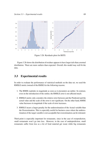
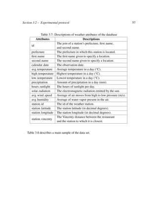
ogenous variables (For more details, see Appendix A). Figure 3.24 shows that the residues
are approximately normally distributed. There does not appear to be a model for the resid-
uals, but there are some outliers. Overall, we find that this model has been successful in
capturing the patterns in the data.

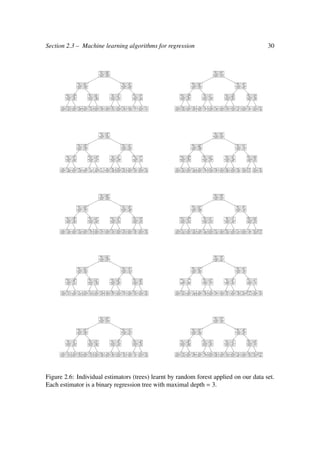
Figure 3.24: ACF, PACF and residuals plots for SARIMAX
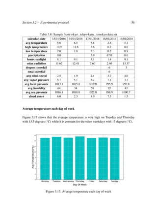
The results are mentioned in Table 3.15.
Table 3.15: Sarimax model results
Statespace Model Results
Dep. Variable: y No. Observations: 93
Model: SARIMAX(2, 0, 0, 7) Log Likelihood -328.688
Date: Friday, 05 June 2020 AIC 665.375
Time: 20:15:00 BIC 674.853
Sample: 0 HQIC 669.172
-93
Covariance Type: opg
coef std err z P > |z| [0.025 0.975]
intercept 5.9385 4.353 1.364 0.173 -2.594 14.471
ar.S.L7 0.5044 0.104 4.871 0.000 0.301 0.707
ar.S.L14 0.3530 0.125 2.827 0.005 0.108 0.598
sigma2 240.6486 28.682 8.390 0.000 184.433 296.864
Ljung-Box (Q): 15.53 Jarque-Bera (JB): 9.36
Prob(Q): 1.00 Prob(JB): 0.01
Heteroskedasticity (H): 1.13 Skew: -0.20
Prob(H) (two-sided): 0.75 Kurtosis: 4.64

The model coefficients are different. Interestingly, the statsmodels implementation
has a lower AIC even though both model have the same order and seasonal order.
Bayesian Structural Time Series (BSTS) model
The BSTS is another time series model that can handle seasonality (See Appendix A).
There is no method to automatically fit the best BSTS model, but we can use the best
SARIMAX model found to fit a BSTS model. This model has:
• An auto-regressive component with a degree of parameter, which should be equiv-
alent to p found for SARIMAX (the first value in order).
• A seasonality component with a parameter period, which should be equivalent to m
for SARIMAX (the last value in seasonal order).
Figure 3.25 shows that there is no significant time lag. Also, there does not appear to be
a trend in the residuals, although they do appear to increase in variance.
Figure 3.25: ACF, PACF and residuals plots for BSTS

Section 3.3 – Experimental results 69
Figure 3.26: Residuals plots for BSTS
Figure 3.26 shows the distribution of residues appears to have larger tails than a normal
distribution. There are more outliers than expected. Overall, this model may well fit the
data.
3.3 Experimental results
In order to evaluate the performance of statistical methods on the data set, we used the
RMSLE metric instead of the RMSE for the following reasons:
1. The RMSE explodes in magnitude as soon as it encounters an outlier. In contrast,
even on the introduction of the outlier, the RMSLE error is not affected much.
2. RMSLE metric only considers the relative error between and the Predicted and the
actual value and the scale of the error is not significant. On the other hand, RMSE
value Increases in magnitude if the scale of error increases.
3. RMSLE incurs a larger penalty for the underestimation of the Actual variable than
the Overestimation. This is especially useful for business cases where the underes-
timation of the target variable is not acceptable but overestimation can be tolerated.
Third point is especially important for restaurants, since in the case of overprediction,
small restaurants won’t go into loss. However, in the case of underprediction, small
restaurants suffer from loss as a lot of food material get waste while big restaurants

Section 3.3 – Experimental results 70
have tolerance for both overprediction and underprediction and RMSLE penalizes under-
predictions more than over-prediction, which is a plus point for small restaurants as japan
has a large no of small restaurants. A lower value of RMSLE corresponds to a better
model. The results of measuring the performance of statistical and machine learning
methods are presented in Table 3.17.
Table 3.16: Results of performance measurement for statistical and machine learning
methods
R-squared MAE MAPE MSE RMSLE
Statistical methods
Regression model 0.281 8.920 71.101 192.444 0.606
AR model 0.272 9.298 73.502 195.340 0.627
MA model 0.268 9.310 73.771 196.358 0.630
ARMA model 0.290 8.875 70.440 191.300 0.602
ARIMA model 0.291 8.868 70.355 191.140 0.601
SARIMAX model 0.387 8.405 66.763 170.230 0.565
BSTS model 0.250 9.781 75.000 198.780 0.691
Machine learning methods
SGD Regressor 0.499 7.651 62.447 168.079 0.532
KNeighbors Regressor 0.569 7.053 61.020 144.688 0.520
Decision Tree Regressor 0.586 6.987 60.326 138.995 0.508
Random Forest Regressor 0.595 6.843 59.574 136.067 0.502
XGB Regressor (GBDT) 0.610 6.495 55.878 130.962 0.484
With reference to the results concluded from the practical experience, one can con-
clude that Seasonal ARIMA with eXogenousregressors (SARIMAX) models give better
results compared to other statistical methods. For example, SARIMAX has the lowest
RMSLE of 0.565 for the data set. Another conclusion deduced from our research is
that the comparison of machine learning methods allowed us to conclude that Gradient
Boosted Decision Trees (GBDT) gives the most adequate values. For instance, GBDT
has the lowest RMSLE value, which is equal to 0.484.
For this particular data set, it can be concluded that machine learning methods have
better results in predicting future visitors of restaurants.
Table 3.17 presents a sample of the number of predicted visitors for a Japanese restau-
rant on future dates with GBDT.

Section 3.4 – Towards Tunisian data 71
Table 3.17: Sample of the future number of visitors for a restaurant with GBDT
visit date visit day name visitors
23/04/2017 Sunday 1.8368614
24/04/2017 Monday 22.002846
25/04/2017 Tuesday 25.21556
26/04/2017 Wednesday 30.953348
27/04/2017 Thursday 31.05272
28/04/2017 Friday 38.33501
29/04/2017 Saturday 11.460871
30/04/2017 Sunday 1.9295475
01/05/2017 Monday 21.318165
02/05/2017 Tuesday 21.829174
3.4 Towards Tunisian data
In this master thesis, we used real reservation data from a Tunisian restaurant detailed
from the RESERV platform, which was extracted and provided as a data set. This data
was issued from the 27th May 2020 to the 6th of September 2020. The focus is on the
use of reservation data, the number of visitors as well as holidays in order to predict the
actual number of visitors that a restaurant will have on a given day.
Due to the particular circumstances that occurred in our country and worldwide, the
collection of data was a little bit diﬃcult, this is why we plan to collect a large amount of
data in order to obtain better forecasts by our model.
3.5 Conclusion
This Chapter highlights the importance of using internal data such as historical visits, his-
torical reservations, restaurant information and external data such as weather and holidays
to estimate how many future visitors will go to a restaurant using statistical analysis and
supervised machine learning algorithms. The evaluation results show the eﬀectiveness of
our approach, as well as useful insights for future work.

Conclusion and future works
Revenue management is an area that has matured over the past 50 years. It started to
be employed as a newly discovered method by Littlewood in the 1970s. Nowadays, it
is becoming more frequently used. It faces the rapid development of forecasting and
optimization in several sectors including the restaurant industry, using Machine Learning
techniques to process the huge amounts of reservation/visitor data that is created every
second.
Today’s Artificial Intelligence and Machine Learning solutions offer many possibili-
ties to optimize and automate processes, save money, and reduce human error for many
restaurants. There are several applications in food service industry that can help predict
visitor traffic, food orders, and inventory needs relevant to forecasting the number of or-
ders needed for a certain period. These applications and solutions allow the collection of
past data to further engage customers by examining their habits and preferences, resulting
in more repetitive visits and orders. These include ”Cloud Big Data” solutions, restau-
rant management platforms that facilitate the payment process and applications that allow
customers to connect and pre-order a place in a restaurant in advance.
In this master dissertation, the first chapter presents the theoretical aspects of yield
and revenue management with their systems and provides a clarification of the different
methods used to predict yield management through statistical methods such as ARIMA
and SARIMAX. Afterwards, this research project focuses on practical aspects by ap-
plying different supervised machine learning algorithms for regression on our database
of restaurants in Japan including information on restaurants, historical tours, historical
reservations, vacation days and historical weather information. We noticed that it is fea-
sible to forecast the number of visitors for restaurants in future dates. Our model gen-
erates predictions by performing regression using Decision Tree, Random Forests, K-
Nearest-Neighbour, Stochastic Gradient Descent and Gradient Boosted Decision Trees
algorithms. Compared to techniques such as Deep Learning, these algorithms have a
relatively low computational cost, so the restaurant owner can deploy them on common
72

Conclusion and future works 73
computers. Then, we tested and compared the statistical and machine learning methods
and concluded that the machine learning methods can perform better with our model.
Beyond the characteristics taken into account by our approach, many factors can facil-
itate the accurate prediction of future restaurant visitors. For example, if a new restaurant
is opened next to an existing restaurant, the number of future visitors to that existing
restaurant may decrease. In addition, social events may bring more visitors to restau-
rants in the aﬀected locations. Therefore, in future work, it is necessary to include more
information in the predictive model, such competitors and social events.
For the case of the reservation data for the Tunisian restaurant explained in Section
3.4, we will continue with the integration of our model with the RESERV platform to
obtain better predictions. We will also try to collect external data such as weather, social
events, etc in order to optimize the results.

Appendix A
Statistical methods for forecasting
A.1 Introduction
In this appendix, different statistical forecasting methods are presented that will be tested
to find the best method for our model.
This appendix is organized as follows: Section A.2 presents stationary analysis, Sec-
tion A.3 presents Seasonal Autoregressive Integrated Moving Average (SARIMA) mod-
els, Section A.4 presents Seasonal AutoRegressive Integrated Moving Average with eX-
ogenous regressors (SARIMAX) models and Section A.5 presents Bayesian Structural
Time Series (BSTS) models.
A.2 Stationary Analysis
Definition A.1. Formally, AR(p) model is represented as (Box and Jenkins, 1976):
εt = φ(L) yt (A.1)
where:
• φ(L) = 0 is the characteristic equation for the model;
• yt is the actual value at time period t;
A necessary and sufficient condition for the AR(p) model to be stationary is that all the
roots of the characteristic equation must fall outside the unit circle. (Hipel and McLeod,
74

Section A.3 – SARIMA models 75
1994) mentioned another simple algorithm by (Pagano, 1973) for determining stationarity
of an AR model.
Example A.1. As shown in the AR(1) model: yt = c + φ1yt−1 + εt is stationary when
|φ1| < 1, with
a constant mean µ =
c
1 − φ1
;
a constant variance γ0 =
σ2
1 − φ2
1
;
(A.2)
An MA(q) model is always stationary, irrespective of the values the MA parameters
(Hipel and McLeod, 1994). The conditions regarding stationarity and invertibility of AR
and MA models also hold for an ARMA model.
An ARMA(p, q) model is stationary if all the roots of the characteristic equation A.3
lie outside the unit circle.
φ(L) = 0 (A.3)
Similarly, if all the roots of the lag equation φ(L) = 0 lie outside the unit circle, then the
ARMA(p, q) model is invertible and can be expressed as a pure AR model.
A.3 Seasonal Autoregressive Integrated Moving Average
(SARIMA) models
(Box and Jenkins, 1976) have generalized ARIMA model to deal with seasonality. Their
proposed model is known as the Seasonal ARIMA (SARIMA) model. SARIMA is gener-
ally referred to as S ARIMA(p, d, q)x(P, D, Q)s, where p, d, q and P, D, Q are non-negative
integers that refer to the polynomial order of the autoregressive (AR), integrated (I), and
moving average (MA) parts of the non-seasonal and seasonal components of the model,
respectively.
Deﬁnition A.2. (SARIMA) Formally, the SARIMA model is:
Φp(B)ΦP(Bs
) d D
s yt = Θq(B)ΘQ(Bs
)εt (A.4)
where:
• yt is the forecast variable (i.e. future number of visitors in restaurant);

Section A.4 – SARIMAX models 76
• Φp(B) is the regular AR polynomial of order p;
• Θq(B) is the regular MA polynomial of order q;
• ΦP(Bs
) is the seasonal AR polynomial of order P;
• ΘQ(Bs
) is the seasonal MA polynomial of order Q;
• The differentiating operator d
and the seasonal differentiating operator D
s elimi-
nate the non-seasonal and seasonal non-stationarity, respectively;
• B is the backshift operator, which operates on the observation yt by shifting it one
point in time (i.e. Bk
(yt) = yt−k );
• εt follows a white noise process;
• s defines the seasonal period;
The polynomials and all operators are defined as follows:
Φp(B) = 1 −
p
i=1
ΦiBi
Φp(Bs
) = 1 −
p
i=1
ΦiBs,i
Θq(B) = 1 −
q
i=1
θiBi
ΘQ(Bs
) = 1 −
Q
i=1
ΘiBs,i
d = (1 − B)d D
s = (1 − Bs
)D
A.4 Seasonal AutoRegressive Integrated Moving Average
with eXogenous regressors (SARIMAX) models
S ARIMAX model is an extension of the S ARIMA model (Box and Jenkins, 1976), en-
hanced with the ability to integrate exogenous (explanatory) variables, in order to increase
its forecasting performance.
Definition A.3. (SARIMAX) This multivariate version of S ARIMA model,called S easonal
ARIMA with eXogenous factor (S ARIMAX), is generally expressed as:
Φp(B)Φp(Bs
) d D
s yt = βk xk,t + θq(B)ΘQ(Bs
)εt (A.5)
where
• xk,t is the vector including the kth
explanatory input variables at time t;

Section A.5 – BSTS models 77
• βk is the coefficient value of the kth
exogenous input variable;
The stationarity and invertibility conditions are equal to those of ARMA models.
A.5 Bayesian Structural Time Series (BSTS) models
Bayesian statistics has been applied to many statistical fields such as regression, classifi-
cation, clustering and time series analysis (Galbraith et al., 2001).
Definition A.4. (BSTS) Bayesian statistics are based on the Bayes theorem as follows
(Faraway and Chatfield, 1998; Suykens and Vandewalle, 1999):
P(θ | x) =
P(x | θ)P(θ)
P(x)
(A.6)
where:
• x is observed data;
• θ is model parameter;
P(x) is computed as follows:
P(x) =
θ
P(x, θ) =
θ
P(x | θ)P(θ). (A.7)
where:
• P(θ) represents the prior function;
• P(x | θ) represents likelihood function;
• P(θ) is the posterior function;
A.6 Conclusion
In this Appendix, we have explained statistical methods that will be used to predict future
restaurant visitor numbers. These methods will be compared using the evaluation metric
in order to find the best method for our forecasting model.

References
Amit, Y. and Geman, D. (1997). Shape quantization and recognition with randomized
trees. Neural computation, 9(7):1545–1588.
Berman, B. (2005). Applying yield management pricing to your service business. Busi-
ness Horizons, 48(2):169–179.
Box, G. E. and Jenkins, G. M. (1976). Time series analysis: Forecasting and control.
Calif: Holden-Day.
Breiman, L. (2001). Random forests. Machine learning, 45(1):5–32.
Capiez, A. (2003). Yield management: optimisation du revenu dans les services. Hermès
Science.
Capiez, A. and Kaya, A. (2004). Yield management and performance in the hotel industry.
Journal of Travel and Tourism Marketing, 16(4):21–31.
Cochrane, J. H. (2005). Time series for macroeconomics and finance. Manuscript, Uni-
versity of Chicago, pages 1–136.
Cross, R. (1997). Revenue Management: Hard-core Tactics for Market Domination.
Broadway Books.
De’Ath, G. (2007). Boosted trees for ecological modeling and prediction. Ecology,
88(1):243–251.
Dennis Jr, J. E. and Schnabel, R. B. (1996). Numerical methods for unconstrained opti-
mization and nonlinear equations. SIAM.
Faraway, J. and Chatfield, C. (1998). Time series forecasting with neural networks: a
comparative study using the air line data. Journal of the Royal Statistical Society:
Series C (Applied Statistics), 47(2):231–250.
78

REFERENCES 79
Friedman, J., Hastie, T., and Tibshirani, R. (2001). The elements of statistical learning,
volume 1. Springer series in statistics New York.
Friedman, J. H. (2002). Stochastic gradient boosting. Computational statistics & data
analysis, 38(4):367–378.
Galbraith, J. W., Zinde-Walsh, V., et al. (2001). Autoregression-based estimators for
arfima models. Technical report, CIRANO.
Gandomi, A. and Haider, M. (2015). Beyond the hype: Big data concepts, methods, and
analytics. International journal of information management, 35(2):137–144.
Haensel, A., Mederer, M., and Schmidt, H. (2011). Revenue management in the car
rental industry: A stochastic programming approach. Journal of Revenue and Pricing
Management, 11.
Hamzaçebi, C. (2008). Improving artificial neural networks’ performance in seasonal
time series forecasting. Information Sciences, 178(23):4550–4559.
Hipel, K. W. and McLeod, A. I. (1994). Time series modelling of water resources and
environmental systems. Elsevier.
Jallat, F. and Ancarani, F. (2008). Yield management, dynamic pricing and crm in
telecommunications. Journal of Services Marketing.
Kimes, S., Chase, R., Choi, S., Lee, P., and Ngonzi, E. (1998). Restaurant revenue man-
agement: Applying yield management to the restaurant industry. Cornell Hotel and
Restaurant Administration Quarterly, 39(3):32–39.
Kimes, S. E. (1999). Implementing restaurant revenue management: A five-step ap-
proach. Cornell Hotel and Restaurant Administration Quarterly, 40(3):16–21.
Lasek, A., Cercone, N., and Saunders, J. (2016). Smart restaurants: Survey on customer
demand and sales forecasting. In Smart Cities and Homes, pages 361–386. Elsevier.
Nair, S. K. and Bapna, R. (2001). An application of yield management for internet service
providers. Naval Research Logistics (NRL), 48(5):348–362.
Pagano, M. (1973). When is an altoregressive scheme stationary. Communications in
Statistics-Theory and Methods, 1(6):533–544.
Rumelhart, D. E., Hinton, G. E., and Williams, R. J. (1985). Learning internal represen-
tations by error propagation. Technical report, California Univ San Diego La Jolla Inst
for Cognitive Science.

REFERENCES 80
Saha, D., Alluri, P., and Gan, A. (2015). Prioritizing highway safety manual’s crash
prediction variables using boosted regression trees. Accident Analysis & Prevention,
79:133–144.
Suhud, U. and Wibowo, A. (2016). Predicting customers’ intention to revisit a vintage-
concept restaurant. Journal of Consumer Sciences, 1(2):56–69.
Suykens, J. A. and Vandewalle, J. (1999). Least squares support vector machine classi-
ﬁers. Neural processing letters, 9(3):293–300.
Talluri, K. T. and Van Ryzin, G. J. (2006). The theory and practice of revenue manage-
ment, volume 68. Springer Science & Business Media.
Taneja, N. K. (1979). Airline traﬃc forecasting; a regression analysis approach.
Vapnik, V. N. and Chervonenkis, A. Y. (2015). On the uniform convergence of relative
frequencies of events to their probabilities. In Measures of complexity, pages 11–30.
Springer.
Witt, S. F., Witt, C. A., et al. (1992). Modeling and forecasting demand in tourism.
Academic Press Ltd.
Zhang, G. P. (2003). Time series forecasting using a hybrid arima and neural network
model. Neurocomputing, 50:159–175.

Résumé
Pour une stratégie efficace et économique, les restaurateurs doivent estimer avec
précision le nombre de leurs futurs visiteurs. Dans ce rapport, nous proposons une ap-
proche pour prédire le nombre de futurs visiteurs pour les restaurants en utilisant des
méthodes statistiques telles que ARIMA, SARIMAX et BSTS et des algorithmes de
régression par Apprentissage Automatique. Notre modèle a comme entrée des données
internes sur des restaurant, des visites historiques, des réservations historiques et des
données externes telles que les jours de vacances et les historiques de température. À par-
tir de ces grands ensembles de données et des informations temporelles, nous avons con-
struit quatre groupes de caractéristiques en conséquence. À partir de ces caractéristiques,
notre approche génère des prévisions en effectuant une régression à l’aide des différents
algorithmes tels que l’Arbre de Décision, les Forêts Aléatoires, le Voisin le Plus Proche
(KNN), la Descente Stochastique par Gradient et les Arbres de Décision à Gradient Aug-
menté (GBDT). Les résultats de l’évaluation montrent l’efficacité de notre approche, ainsi
que les indications utiles pour un futur projet de recherche.
Mots clés
Intelligence Artificielle, Apprentissage Automatique, Informatique Décisionnelle,
Prévision, Restaurant, Gestion du Rendement, Analyse Statistique.
Abstract
For an effective and economical strategy, restaurant owners must accurately estimate
the number of their future visitors. In this report, we propose an approach for predicting
the number of future visitors for restaurants using statistical methods such as ARIMA,
SARIMAX and BSTS and machine learning regression algorithms. Our model has as in-
put internal restaurant data, historical visits, historical reservations and external data such
as vacation days and temperature histories. From these large data sets and time informa-
tion, we constructed four groups of characteristics accordingly. Using these characteris-
tics, our approach generates forecasts by performing regression using different algorithms
such as Decision Tree, Random Forests, K-Nearest-Neighbour, Stochastic Gradient De-
scent and Gradient Boosted Decision Trees. The results of the evaluation show the effec-
tiveness of our approach, as well as the useful indications for a future research project.
Keywords
Artificial Intelligence, Machine Learning, Business Intelligence, Forecasting, Restaurant,
Yield Management, Statistical Analysis.

Applying Machine Learning Techniques to Revenue Management

More Related Content

What's hot

Similar to Applying Machine Learning Techniques to Revenue Management

Recently uploaded

Applying Machine Learning Techniques to Revenue Management