The physics-of-solar-cells-ch-1

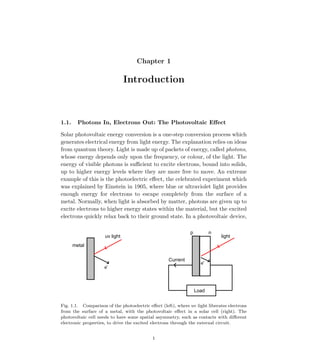
March 12, 2003 15:18 WSPC/The Physics of Solar Cells psc
Chapter 1
Introduction
1.1. Photons In, Electrons Out: The Photovoltaic Effect
Solar photovoltaic energy conversion is a one-step conversion process which
generates electrical energy from light energy. The explanation relies on ideas
from quantum theory. Light is made up of packets of energy, called photons,
whose energy depends only upon the frequency, or colour, of the light. The
energy of visible photons is sufficient to excite electrons, bound into solids,
up to higher energy levels where they are more free to move. An extreme
example of this is the photoelectric effect, the celebrated experiment which
was explained by Einstein in 1905, where blue or ultraviolet light provides
enough energy for electrons to escape completely from the surface of a
metal. Normally, when light is absorbed by matter, photons are given up to
excite electrons to higher energy states within the material, but the excited
electrons quickly relax back to their ground state. In a photovoltaic device,
1. Introduction
1.1 Photons in, electrons out: The Photovoltaic effect
Solar photovoltaic energy conversion is a one-step conversion process which generates electrical energy
from light energy. The explanation relies on ideas from quantum theory. Light is made up of packets of
energy, called photons, whose energy depends only upon the frequency, or colour, of the light. The
energy of visible photons is sufficient to excite electrons, bound into solids, up to higher energy levels
where they are more free to move. An extreme example of this is the photoelectric effect, the celebrated
experiment which was explained by Einstein in 1905, where blue or ultraviolet light provides enough
energy for electrons to escape completely from the surface of a metal. Normally, when light is absorbed
by matter, photons are given up to excite electrons to higher energy states within the material, but the
excited electrons quickly relax back to their ground state. In a photovoltaic device, however, there is
some built-in asymmetry which pulls the excited electrons away before they can relax, and feeds them
them to an external circuit. The extra energy of the excited electrons generates a potential difference, or
electro-motive force (e.m.f.). This force drives the electrons through a load in the external circuit to do
electrical work.
e-
e-
Load
p n
Current
uv light light
metal
Figure 1.1 Comparison of the photoelectric effect (left), where uv light liberates electrons from the surface of a metal, with the
photovoltaic effect in a solar cell (right). The photovoltaic cell needs to have some spatial asymmetry, such as contacts with
different electronic properties, to drive the excited electrons towards the external circuit.
The effectiveness of a photovoltaic device depends upon the choice of light absorbing materials and the
way in which they are connected to the external circuit. The following chapters will deal with the
underlying physical ideas, the device physics of solar cells, the properties of photovoltaic materials and
solar cell design. In this Chapter we will summarise the main characteristics of a photovoltaic cell
without discussing its physical function in detail.
1.2 Brief history of the solar cell
The photovoltaic effect was first reported by Edmund Bequerel in 1839 when he observed that the
action of light on a silver coated platinum electrode immersed in electrolyte produced an electric
current. Forty years later the first solid state photovoltaic devices were constructed by workers
Fig. 1.1. Comparison of the photoelectric effect (left), where uv light liberates electrons
from the surface of a metal, with the photovoltaic effect in a solar cell (right). The
photovoltaic cell needs to have some spatial asymmetry, such as contacts with different
electronic properties, to drive the excited electrons through the external circuit.
1

2 The Physics of Solar Cells
however, there is some built-in asymmetry which pulls the excited electrons
away before they can relax, and feeds them to an external circuit. The extra
energy of the excited electrons generates a potential difference, or electro-
motive force (e.m.f.). This force drives the electrons through a load in the
external circuit to do electrical work.
The effectiveness of a photovoltaic device depends upon the choice of
light absorbing materials and the way in which they are connected to the
external circuit. The following chapters will deal with the underlying phys-
ical ideas, the device physics of solar cells, the properties of photovoltaic
materials and solar cell design. In this chapter we will summarise the main
characteristics of a photovoltaic cell without discussing its physical function
in detail.
1.2. Brief History of the Solar Cell
The photovoltaic effect was first reported by Edmund Bequerel in 1839
when he observed that the action of light on a silver coated platinum elec-
trode immersed in electrolyte produced an electric current. Forty years
later the first solid state photovoltaic devices were constructed by work-
ers investigating the recently discovered photoconductivity of selenium. In
1876 William Adams and Richard Day found that a photocurrent could
be produced in a sample of selenium when contacted by two heated plat-
inum contacts. The photovoltaic action of the selenium differed from its
photoconductive action in that a current was produced spontaneously by
the action of light. No external power supply was needed. In this early pho-
tovoltaic device, a rectifying junction had been formed between the semi-
conductor and the metal contact. In 1894, Charles Fritts prepared what
was probably the first large area solar cell by pressing a layer of selenium
between gold and another metal. In the following years photovoltaic effects
were observed in copper–copper oxide thin film structures, in lead sulphide
and thallium sulphide. These early cells were thin film Schottky barrier
devices, where a semitransparent layer of metal deposited on top of the
semiconductor provided both the asymmetric electronic junction, which is
necessary for photovoltaic action, and access to the junction for the inci-
dent light. The photovoltaic effect of structures like this was related to the
existence of a barrier to current flow at one of the semiconductor–metal
interfaces (i.e., rectifying action) by Goldman and Brodsky in 1914. Later,
during the 1930s, the theory of metal–semiconductor barrier layers was
developed by Walter Schottky, Neville Mott and others.

Introduction 3
However, it was not the photovoltaic properties of materials like sele-
nium which excited researchers, but the photoconductivity. The fact that
the current produced was proportional to the intensity of the incident light,
and related to the wavelength in a definite way meant that photoconductive
materials were ideal for photographic light meters. The photovoltaic effect
in barrier structures was an added benefit, meaning that the light meter
could operate without a power supply. It was not until the 1950s, with the
development of good quality silicon wafers for applications in the new solid
state electronics, that potentially useful quantities of power were produced
by photovoltaic devices in crystalline silicon.
In the 1950s, the development of silicon electronics followed the discov-
ery of a way to manufacture p–n junctions in silicon. Naturally n type silicon
wafers developed a p type skin when exposed to the gas boron trichloride.
Part of the skin could be etched away to give access to the n type layer
beneath. These p–n junction structures produced much better rectifying
action than Schottky barriers, and better photovoltaic behaviour. The first
silicon solar cell was reported by Chapin, Fuller and Pearson in 1954 and
converted sunlight with an efficiency of 6%, six times higher than the best
previous attempt. That figure was to rise significantly over the following
years and decades but, at an estimated production cost of some $200 per
Watt, these cells were not seriously considered for power generation for sev-
eral decades. Nevertheless, the early silicon solar cell did introduce the pos-
sibility of power generation in remote locations where fuel could not easily
be delivered. The obvious application was to satellites where the require-
ment of reliability and low weight made the cost of the cells unimportant
and during the 1950s and 60s, silicon solar cells were widely developed for
applications in space.
Also in 1954, a cadmium sulphide p–n junction was produced with an
efficiency of 6%, and in the following years studies of p–n junction pho-
tovoltaic devices in gallium arsenide, indium phosphide and cadmium tel-
luride were stimulated by theoretical work indicating that these materials
would offer a higher efficiency. However, silicon remained and remains the
foremost photovoltaic material, benefiting from the advances of silicon tech-
nology for the microelectronics industry. Short histories of the solar cell are
given elsewhere [Shive, 1959; Wolf, 1972; Green, 1990].
In the 1970s the crisis in energy supply experienced by the oil-dependent
western world led to a sudden growth of interest in alternative sources of
energy, and funding for research and development in those areas. Photo-
voltaics was a subject of intense interest during this period, and a range of

strategies for producing photovoltaic devices and materials more cheaply
and for improving device efficiency were explored. Routes to lower cost in-
cluded photoelectrochemical junctions, and alternative materials such as
polycrystalline silicon, amorphous silicon, other ‘thin film’ materials and
organic conductors. Strategies for higher efficiency included tandem and
other multiple band gap designs. Although none of these led to widespread
commercial development, our understanding of the science of photovoltaics
is mainly rooted in this period.
During the 1990s, interest in photovoltaics expanded, along with grow-
ing awareness of the need to secure sources of electricity alternative to
fossil fuels. The trend coincides with the widespread deregulation of the
electricity markets and growing recognition of the viability of decentralised
power. During this period, the economics of photovoltaics improved pri-
marily through economies of scale. In the late 1990s the photovoltaic pro-
duction expanded at a rate of 15–25% per annum, driving a reduction in
cost. Photovoltaics first became competitive in contexts where conventional
electricity supply is most expensive, for instance, for remote low power ap-
plications such as navigation, telecommunications, and rural electrification
and for enhancement of supply in grid-connected loads at peak use [An-
derson, 2001]. As prices fall, new markets are opened up. An important
example is building integrated photovoltaic applications, where the cost of
the photovoltaic system is offset by the savings in building materials.
1.3. Photovoltaic Cells and Power Generation
1.3.1. Photovoltaic cells, modules and systems
The solar cell is the basic building block of solar photovoltaics. The cell can
be considered as a two terminal device which conducts like a diode in the
dark and generates a photovoltage when charged by the sun. Usually it is a
thin slice of semiconductor material of around 100 cm2
in area. The surface
is treated to reflect as little visible light as possible and appears dark blue
or black. A pattern of metal contacts is imprinted on the surface to make
electrical contact (Fig. 1.2(a)).
When charged by the sun, this basic unit generates a dc photovoltage of
0.5 to 1 volt and, in short circuit, a photocurrent of some tens of milliamps
per cm2
. Although the current is reasonable, the voltage is too small for
most applications. To produce useful dc voltages, the cells are connected to-
gether in series and encapsulated into modules. A module typically contains

Introduction 5
3
voltage which is some multiple of 12V, under standard illumination. For almost all applications the
illumination is too variable for efficient operation all the time and the photovoltaic generator must be
integrated with a charge storage system (a battery) and with components for power regulation
(Fig.1.2(d)). The battery is used to store charge generated during sunny periods and the power
conditioning ensures that the power supply is regular and less sensitive to the solar irradiation. For ac
electrical power, to power ac designed appliances and for integration with an electricity grid, the dc
current supplied by the photovoltaic modules is converted to ac power of appropriate frequency using
an inverter.
The design and engineering of photovoltaic systems is beyond the scope of this book. A more detailed
introduction is given by Markvart [Markvart, 2000] and Lorenzo [Lorenzo, 1994]. Photovoltaic systems
engineering essentially depends upon the electrical characteristics of the individual cells.
+12V
0V
(a) (b)
0
+V
Module
PV generator
Power
Load
Storage
(Battery (dc)
or Grid (ac))
conditioning
Figure 1.2 (a) Photovoltaic cell (b) In a module, cells are connected in series to give a standard dc voltage of 12V (c) For any
application, modules are connected in series and parallel into an array, which produces sufficient current and voltage to meet the
demand. (d) In most cases the photovoltaic array should be integrated with components for charge regulation and storage.
1.3.2. Some important definitions
load
solar cell
load
battery
A B
Figure 1.3 The solar cell may replace a battery in a simple circuit.
The solar cell can take the place of a battery in a simple electric circuit (Fig. 1.3). In the dark the cell in
circuit A does nothing. When it is switched on by light it develops a voltage, or e.m.f., analogous to the
e.m.f. of the battery in circuit B. The voltage developed when the terminals are isolated (infinite load
resistance) is called the open-circuit voltage Voc . The current drawn when the terminals are connected
together is the short-circuit current Isc. For any intermediate load resistance RL the cell develops a
voltage V between 0 and Voc and delivers a current I such that V = IRL and I(V) is determined by the
current-voltage characteristic of the cell under that illumination. Thus both I and V are determined by
the illumination as well as the load. Since the current is roughly proportional to the illuminated area, the
short circuit current density Jsc is the useful quantity for comparison. These quantities are defined for a
(c) (d)
Fig. 1.2. (a) Photovoltaic cell showing surface contact patterns (b) In a module, cells
are usually connected in series to give a standard dc voltage of 12 V (c) For any appli-
cation, modules are connected in series into strings and then in parallel into an array,
which produces sufficient current and voltage to meet the demand. (d) In most cases
the photovoltaic array should be integrated with components for charge regulation and
storage.
28 to 36 cells in series, to generate a dc output voltage of 12 V in stan-
dard illumination conditions (Fig. 1.2(b)). The 12 V modules can be used
singly, or connected in parallel and series into an array with a larger current
and voltage output, according to the power demanded by the application
(Fig. 1.2(c)). Cells within a module are integrated with bypass and blocking
diodes in order to avoid the complete loss of power which would result if one

cell in the series failed. Modules within arrays are similarly protected. The
array, which is also called a photovoltaic generator, is designed to generate
power at a certain current and a voltage which is some multiple of 12 V,
under standard illumination. For almost all applications, the illumination is
too variable for efficient operation all the time and the photovoltaic gener-
ator must be integrated with a charge storage system (a battery) and with
components for power regulation (Fig. 1.2(d)). The battery is used to store
charge generated during sunny periods and the power conditioning ensures
that the power supply is regular and less sensitive to the solar irradiation.
For ac electrical power, to power ac designed appliances and for integration
with an electricity grid, the dc current supplied by the photovoltaic modules
is converted to ac power of appropriate frequency using an inverter.
The design and engineering of photovoltaic systems is beyond the scope
of this book. A more detailed introduction is given by Markvart [Markvart,
2000] and Lorenzo [Lorenzo, 1994]. Photovoltaic systems engineering de-
pends to a large degree upon the electrical characteristics of the individual
cells.
The solar cell can take the place of a battery in a simple electric circuit
(Fig. 1.3). In the dark the cell in circuit A does nothing. When it is switched
on by light it develops a voltage, or e.m.f., analogous to the e.m.f. of the
battery in circuit B. The voltage developed when the terminals are isolated
(infinite load resistance) is called the open circuit voltage Voc. The current
drawn when the terminals are connected together is the short circuit cur-
rent Isc. For any intermediate load resistance RL the cell develops a voltage
V between 0 and Voc and delivers a current I such that V = IRL and
I(V ) is determined by the current–voltage characteristic of the cell under
0
+V
Module
PV generator
Power
Load
Storage
( Battery (dc)
or Grid (ac))
conditioning
load
solar cell
load
battery
A B
simple, ideal diode model of a solar cell in section 1.4 below.
(a)
0
+V
Module
PV generator
Power
Load
Storage
( Battery (dc)
or Grid (ac))
conditioning
load
solar cell
load
battery
A B
simple, ideal diode model of a solar cell in section 1.4 below.
(b)
Fig. 1.3. The solar cell may replace a battery in a simple circuit.

Introduction 7
that illumination. Thus both I and V are determined by the illumination
as well as the load. Since the current is roughly proportional to the illumi-
nated area, the short circuit current density Jsc is the useful quantity for
comparison. These quantities are defined for a simple, ideal diode model of
a solar cell in Sec. 1.4 below.
Box 1.1. Solar cell compared with conventional battery
The photovoltaic cell differs from a simple dc battery in these respects:
the e.m.f. of the battery is due to the permanent electrochemical potential
difference between two phases in the cell, while the solar cell derives its
e.m.f. from a temporary change in electrochemical potential caused by light.
The power delivered by the battery to a constant load resistance is relatively
constant, while the power delivered by the solar cell depends on the incident
light intensity, and not primarily on the load (Fig. 1.4). The battery is
completely discharged when it reaches the end of its life, while the solar cell,
although its output varies with intensity, is in principle never exhausted,
since it can be continually recharged with light.
The battery is modelled electrically as a voltage generator and is char-
acterised by its e.m.f. (which, in practice, depends upon the degree of dis-
charge), its charge capacity, and by a polarisation curve which describes
how the e.m.f. varies with current [Vincent 1997]. The solar cell, in con-
trast, is better modelled as a current generator, since for all but the largest
loads the current drawn is independent of load. But its characteristics de-
pend entirely on the nature of the illuminating source, and so Isc and Voc
must be quoted for a known spectrum, usually for standard test conditions
(defined below).
1.4. Characteristics of the Photovoltaic Cell: A Summary
1.4.1. Photocurrent and quantum efficiency
The photocurrent generated by a solar cell under illumination at short cir-
cuit is dependent on the incident light. To relate the photocurrent density,
Jsc, to the incident spectrum we need the cell’s quantum efficiency, (QE).
QE(E) is the probability that an incident photon of energy E will deliver
one electron to the external circuit. Then
Jsc = q
Z
bs(E)QE(E)dE (1.1)

Increasing light intensity
Current
Voltage
Battery
Solar cell
Battery e.m.f.
Fig 1.4
Fig. 1.4. Voltage–current curves of a conventional battery (grey) and a solar cell under
different levels of illumination. A battery normally delivers a constant e.m.f. at different
levels of current drain except for very low resistance loads, when the e.m.f. begins to
fall. The battery e.m.f. will also deteriorate when the battery is heavily discharged. The
solar cell delivers a constant current for any given illumination level while the voltage
is determined largely by the resistance of the load. For photovoltaic cells it is usual to
plot the data in the opposite sense, with current on the vertical axis and voltage on the
horizontal axis. This is because the photovoltaic cell is essentially a current source, while
the battery is a voltage source.
where bs(E) is the incident spectral photon flux density, the number of
photons of energy in the range E to E +dE which are incident on unit area
in unit time and q is the electronic charge. QE depends upon the absorption
coefficient of the solar cell material, the efficiency of charge separation and
the efficiency of charge collection in the device but does not depend on
the incident spectrum. It is therefore a key quantity in describing solar
cell performance under different conditions. Figure 1.5 shows a typical QE
spectrum in comparison with the spectrum of solar photons.
QE and spectrum can be given as functions of either photon energy or
wavelength, λ. Energy is a more convenient parameter for the physics of
solar cells and it will be used in this book. The relationship between E and
λ is defined by
E =
hc
λ
(1.2)
where h is Planck’s constant and c the speed of light in vacuum. A con-
venient rule for converting between photon energies, in electron-Volts, and
wavelengths, in nm, is E/eV = 1240/(λ/nm).

Introduction 9
200 400 600 800 1000 1200 1400 1600 1800
Wavelength / nm
Photon
flux
density
/
a.u.
QE
/
a.u.
QEof gallium arsenide cell
Solar photon flux density
Figure 1.5
Fig. 1.5. Quantum efficiency of GaAs cell compared to the solar spectrum. The vertical
scale is in arbitrary units, for comparison. The short circuit photocurrent is obtained
by integrating the product of the photon flux density and QE over photon energy. It is
desirable to have a high QE at wavelengths where the solar flux density is high.
1.4.2. Dark current and open circuit voltage
When a load is present, a potential difference develops between the termi-
nals of the cell. This potential difference generates a current which acts in
the opposite direction to the photocurrent, and the net current is reduced
from its short circuit value. This reverse current is usually called the dark
current in analogy with the current Idark(V ) which flows across the device
under an applied voltage, or bias, V in the dark. Most solar cells behave
like a diode in the dark, admitting a much larger current under forward
bias (V > 0) than under reverse bias (V < 0). This rectifying behaviour is
a feature of photovoltaic devices, since an asymmetric junction is needed
to achieve charge separation. For an ideal diode the dark current density
Jdark(V ) varies like
Jdark(V ) = Jo(eqV/kBT
− 1) (1.3)
where Jo is a constant, kB is Boltzmann’s constant and T is temperature
in degrees Kelvin.
The overall current voltage response of the cell, its current–voltage char-
acteristic, can be approximated as the sum of the short circuit photocurrent
and the dark current (Fig. 1.6). This step is known as the superposition ap-
proximation. Although the reverse current which flows in reponse to voltage
in an illuminated cell is not formally equal to the current which flows in the
dark, the approximation is reasonable for many photovoltaic materials and

Bias voltage, V
Current
density,
J
Dark current
Jsc
Voc
Light current
Figure 1.6
Fig. 1.6. Current–voltage characteristic of ideal diode in the light and the dark. To
a first approximation, the net current is obtained by shifting the bias dependent dark
current up by a constant amount, equal to the short circuit photocurrent. The sign
convention is such that the short circuit photocurrent is positive.
will be used for the present discussion. The sign convention for current and
voltage in photovoltaics is such that the photocurrent is positive. This is
the opposite to the usual convention for electronic devices. With this sign
convention the net current density in the cell is
J(V ) = Jsc − Jdark(V ) , (1.4)
which becomes, for an ideal diode,
J = Jsc − Jo(eqV/kBT
− 1) . (1.5)
This result is derived in Chapter 6.
When the contacts are isolated, the potential difference has its maximum
value, the open circuit voltage Voc. This is equivalent to the condition when
the dark current and short circuit photocurrent exactly cancel out. For the
ideal diode, from Eq. 1.5,
Voc =
kT
q
ln

Jsc
J0
+ 1

. (1.6)
Equation 1.6 shows that Voc increases logarithmically with light intensity.
Note that voltage is defined so that the photovoltage occurs in forward bias,
where V 0.
Figure 1.6 shows that the current–voltage product is positive, and the
cell generates power, when the voltage is between 0 and Voc. At V 0, the
illuminated device acts as a photodetector, consuming power to generate a

Introduction 11
8
difference between the cell terminals but a smaller current though the load. The diode thus provides the
photovoltage. Without the diode, there is nothing to drive the photocurrent through the load.
Jsc
J
dark
V
+
-
Figure 1.7. Equivalent circuit of ideal solar cell.
1.4.3 Efficiency
The operating regime of the solar cell is the range of bias, from 0 to Voc, in which the cell delivers
power. The cell power density is given by
P JV
= (1.7)
P reaches a maximum at the cell’s operating point or maximum power point. This occurs at some
voltage Vm with a corresponding current density Jm, shown in Fig. 1.8. The optimum load thus has sheet
resistance given by V J
m m . The fill factor is defined as the ratio
FF
J V
J V
m m
sc oc
= (1.8)
and describes the 'squareness' of the
J–V curve.
Fig. 1.7. Equivalent circuit of ideal solar cell.
photocurrent which is light dependent but bias independent. At V Voc,
the device again consumes power. This is the regime where light emitting
diodes operate. We will see later that in some materials the dark current is
accompanied by the emission of light.
Electrically, the solar cell is equivalent to a current generator in parallel
with an asymmetric, non linear resistive element, i.e., a diode (Fig. 1.7).
When illuminated, the ideal cell produces a photocurrent proportional to
the light intensity. That photocurrent is divided between the variable resis-
tance of the diode and the load, in a ratio which depends on the resistance
of the load and the level of illumination. For higher resistances, more of the
photocurrent flows through the diode, resulting in a higher potential differ-
ence between the cell terminals but a smaller current though the load. The
diode thus provides the photovoltage. Without the diode, there is nothing
to drive the photocurrent through the load.
1.4.3. Efficiency
The operating regime of the solar cell is the range of bias, from 0 to Voc, in
which the cell delivers power. The cell power density is given by
P = JV . (1.7)
P reaches a maximum at the cell’s operating point or maximum power
point. This occurs at some voltage Vm with a corresponding current density
Jm, shown in Fig. 1.8. The optimum load thus has sheet resistance given
by Vm/Jm. The fill factor is defined as the ratio
FF =
JmVm
JscVoc
(1.8)
and describes the ‘squareness’ of the J–V curve.

Bias voltage, V
Current
density,
J
Current density
Voc
Jsc
Vm
Jm
Power
density
Maximum
power point
Fig. 1.8
Fig. 1.8. The current voltage (black) and power–voltage (grey) characteristics of an
ideal cell. Power density reaches a maximum at a bias Vm, close to Voc. The maximum
power density Jm × Vm is given by the area of the inner rectangle. The outer rectangle
has area Jsc × Voc. If the fill factor were equal to 1, the current voltage curve would
follow the outer rectangle.
The efficiency η of the cell is the power density delivered at operating
point as a fraction of the incident light power density, Ps,
η =
JmVm
Ps
. (1.9)
Efficiency is related to Jsc and Voc using FF,
η =
JscVocFF
Ps
. (1.10)
These four quantities: Jsc, Voc, FF and η are the key performance char-
acteristics of a solar cell. All of these should be defined for particular il-
lumination conditions. The Standard Test Condition (STC) for solar cells
is the Air Mass 1.5 spectrum, an incident power density of 1000 W m−2
,
and a temperature of 25◦
C. (Standard and other solar spectra are discussed
in Chapter 2.) The performance characteristics for the most common solar
cell materials are listed in Table 1.1.
Table 1.1 shows that solar cell materials with higher Jsc tend to have
lower Voc. This is a consequence of the material used, and particularly of

Introduction 13
Table 1.1. Performance of some types of PV cell [Green et al., 2001].
Cell Type Area (cm2) Voc (V) Jsc (mA/cm2) FF Efficiency (%)
crystalline Si 4.0 0.706 42.2 82.8 24.7
crystalline GaAs 3.9 1.022 28.2 87.1 25.1
poly-Si 1.1 0.654 38.1 79.5 19.8
a-Si 1.0 0.887 19.4 74.1 12.7
CuInGaSe2 1.0 0.669 35.7 77.0 18.4
CdTe 1.1 0.848 25.9 74.5 16.4
10
crystalline GaAs 3.9 1.022 28.2 87.1 25.1
poly-Si 1.1 0.654 38.1 79.5 19.8
a-Si 1.0 0.887 19.4 74.1 12.7
CuInGaSe2 1.0 0.669 35.7 77.0 18.4
Cd Te 1.1 0.848 25.9 74.5 16.4
Table 1.1 shows that solar cell materials with higher Jsc tend to have lower Voc. This is a consequence of
the material used, and particularly of the band gap of the semiconductor. In Chapter 2 we will see that
there is a fundamental compromise between photocurrent and voltage in photovoltaic energy
conversion. Figure 1.9 illustrates the correlation between Jsc and Voc for the cells in Table 1.1, together
with the relationship for a cell of maximum efficiency.
0
10
20
30
40
50
60
70
80
0.5 0.6 0.7 0.8 0.9 1 1.1 1.2
Voc /V
J
sc
/
mA
cm
-2
GaAs
a-Si
CdTe
poly-Si
c-Si
CIGS
theoretical limit
Figure 1.9. Plot of Jsc against Voc for the cells listed in Table 1.1. Materials with high Voc tend of have lower Jsc. This is due to
the band gap of the semiconductor material. The grey line shows the relationship expected in the theoretical limit.
1.4.4 Parasitic resistances
In real cells power is dissipated through the resistance of the contacts and through leakage currents
around the sides of the device. These effects are equivalent electrically to two parasitic resistances in
series (Rs) and in parallel (Rsh) with the cell (Fig. 1.9).
Jsc
Jdark
V
+
-
R
Rsh
s
Fig 1.9. Equivalent circuit including series and shunt resistances.
Fig. 1.9. Plot of Jsc against Voc for the cells listed in Table 1.1. Materials with high
Voc tend to have lower Jsc. This is due to the band gap of the semiconductor material.
The grey line shows the relationship expected in the theoretical limit.
the band gap of the semiconductor. In Chapter 2 we will see that there is a
fundamental compromise between photocurrent and voltage in photovoltaic
energy conversion. Figure 1.9 illustrates the correlation between Jsc and
Voc for the cells in Table 1.1, together with the relationship for a cell of
maximum efficiency.
1.4.4. Parasitic resistances
In real cells power is dissipated through the resistance of the contacts and
through leakage currents around the sides of the device. These effects are

10
Voc /V
Figure 1.9. Plot of Jsc against Voc for the cells listed in Table 1.1. Materials with high Voc tend of have lower Jsc. This is due to
the band gap of the semiconductor material. The grey line shows the relationship expected in the theoretical limit.
1.4.4 Parasitic resistances
In real cells power is dissipated through the resistance of the contacts and through leakage currents
around the sides of the device. These effects are equivalent electrically to two parasitic resistances in
series (Rs) and in parallel (Rsh) with the cell (Fig. 1.9).
Jsc
Jdark
V
+
-
R
Rsh
s
Fig 1.9. Equivalent circuit including series and shunt resistances.
Fig. 1.10. Equivalent circuit including series and shunt resistances.
The series resistance arises from the resistance of the cell material to current flow, particularly through
the front surface to the contacts, and from resistive contacts. Series resistance is a particular problem at
high current densities, for instance under concentrated light. The parallel or shunt resistance arises from
leakage of current through the cell, around the edges of the device and between contacts of different
polarity. It is a problem in poorly rectifying devices.
(a)
Bias
Current
Rs increasing
(b)
Bias
Current
Rsh decreasing
Figure 1.10: Effect of (a) increasing series and (b) reducing parallel resistances. In each case the outer curve has Rs = 0
and Rsh = ∞. In each case the effect of the resistances is to reduce the area of the maximum power rectangle compared to Jsc ×
Voc.
Series and parallel resistances reduce the fill factor as shown in Fig. 1.10. For an efficient cell we want
Rs to be as small and Rsh to be as large as possible.
When parasitic resistances are included the diode equation becomes
J J J e
V JAR
R
sc o
q V JAR kT s
sh
s
= − − −
+
+
( )
( )/
1 . (1.11)
1.4.5 Non-ideal diode behaviour
The ‘ideal’ diode behaviour of eqn. 1.5 is seldom seen. It is common for the dark current to depend
more weakly on bias. The actual dependence on V is quantified by an ideality factor, m and the current–
voltage characteristic given by the non-ideal diode equation,
J J J e
sc o
qV mk T
B
= − −
( )
/
1 (1.12)
m typically lies between 1 and 2. The reasons for non-ideal behaviour will be discussed in later
chapters.
1.5 Summary of Chapter 1
A photovoltaic cell consists of a light absorbing material which is connected to an external circuit in an
asymmetric manner. Charge carriers are generated in the material by the absorption of photons of light,
and are driven towards one or other of the contacts by the built-in spatial asymmetry. This light driven
charge separation establishes a photovoltage at open circuit, and generates a photocurrent at short
circuit. When a load is connected to the external circuit the cell produces both current and voltage and
can do electrical work.
(a)
The series resistance arises from the resistance of the cell material to current flow, particularly through
the front surface to the contacts, and from resistive contacts. Series resistance is a particular problem at
high current densities, for instance under concentrated light. The parallel or shunt resistance arises from
leakage of current through the cell, around the edges of the device and between contacts of different
polarity. It is a problem in poorly rectifying devices.
(a)
Bias
Current
Rs increasing
(b)
Bias
Current
Rsh decreasing
Figure 1.10: Effect of (a) increasing series and (b) reducing parallel resistances. In each case the outer curve has Rs = 0
and Rsh = ∞. In each case the effect of the resistances is to reduce the area of the maximum power rectangle compared to Jsc ×
Voc.
Series and parallel resistances reduce the fill factor as shown in Fig. 1.10. For an efficient cell we want
Rs to be as small and Rsh to be as large as possible.
When parasitic resistances are included the diode equation becomes
J J J e
V JAR
R
sc o
q V JAR kT s
sh
s
= − − −
+
+
( )
( )/
1 . (1.11)
1.4.5 Non-ideal diode behaviour
The ‘ideal’ diode behaviour of eqn. 1.5 is seldom seen. It is common for the dark current to depend
more weakly on bias. The actual dependence on V is quantified by an ideality factor, m and the current–
voltage characteristic given by the non-ideal diode equation,
J J J e
sc o
qV mk T
B
= − −
( )
/
1 (1.12)
m typically lies between 1 and 2. The reasons for non-ideal behaviour will be discussed in later
chapters.
1.5 Summary of Chapter 1
A photovoltaic cell consists of a light absorbing material which is connected to an external circuit in an
asymmetric manner. Charge carriers are generated in the material by the absorption of photons of light,
and are driven towards one or other of the contacts by the built-in spatial asymmetry. This light driven
charge separation establishes a photovoltage at open circuit, and generates a photocurrent at short
circuit. When a load is connected to the external circuit the cell produces both current and voltage and
can do electrical work.
(b)
Fig. 1.11. Effect of (a) increasing series and (b) reducing parallel resistances. In each
case the outer curve has Rs = 0 and Rsh = ∞. In each case the effect of the resistances
is to reduce the area of the maximum power rectangle compared to Jsc × Voc.
equivalent electrically to two parasitic resistances in series (Rs) and in par-
allel (Rsh) with the cell (Fig. 1.10).
The series resistance arises from the resistance of the cell material to
current flow, particularly through the front surface to the contacts, and
from resistive contacts. Series resistance is a particular problem at high
current densities, for instance under concentrated light. The parallel or
shunt resistance arises from leakage of current through the cell, around
the edges of the device and between contacts of different polarity. It is a
problem in poorly rectifying devices.
Series and parallel resistances reduce the fill factor as shown in Fig. 1.11.
For an efficient cell we want Rs to be as small and Rsh to be as large as
possible.
When parasitic resistances are included, the diode equation becomes
J = Jsc − Jo(eq(V+JARs)/kT
− 1) −
V + JARs
Rsh
. (1.11)

Introduction 15
1.4.5. Non-ideal diode behaviour
The ‘ideal’ diode behaviour of Eq. 1.5 is seldom seen. It is common for the
dark current to depend more weakly on bias. The actual dependence on V
is quantified by an ideality factor, m and the current–voltage characteristic
given by the non-ideal diode equation,
J = Jsc − Jo(eqV/mkBT
− 1) (1.12)
m typically lies between 1 and 2. The reasons for non-ideal behaviour will
be discussed in later chapters.
1.5. Summary
A photovoltaic cell consists of a light absorbing material which is connected
to an external circuit in an asymmetric manner. Charge carriers are gener-
ated in the material by the absorption of photons of light, and are driven
towards one or other of the contacts by the built-in spatial asymmetry. This
light driven charge separation establishes a photovoltage at open circuit,
and generates a photocurrent at short circuit. When a load is connected to
the external circuit, the cell produces both current and voltage and can do
electrical work.
The size of the current generated by the cell in short circuit depends
upon the intensity and the energy spectrum of the incident light. Photocur-
rent is related to incident spectrum by the quantum efficiency of the cell,
which is the probability of generating an electron per incident photon as a
function of photon energy. When a load is present, a potential difference is
created between the terminals of the cell and this drives a current, usually
called the dark current, in the opposite direction to the photocurrent. As
the load resistance is increased, the potential difference increases and the
net current decreases until the photocurrent and dark current exactly cancel
out. The potential difference at this point is called the open circuit voltage.
At some point before Voc is reached, the current–voltage product is max-
imum. This is the maximum power point and the cell should be operated
with a load resistance which corresponds to this point.
The solar cell can be modelled as a current generator in parallel with an
ideal diode, and the current–voltage characteristic given by the ideal diode
equation, Eq. 1.5. In real cells, the behaviour is degraded by the presence
of series and parallel resistances.

References
D. Anderson, Clean Electricity from Photovoltaics, eds. M.D. Archer and R.D.
Hill (London: Imperial College Press, 2001).
M.A. Green, “Photovoltaics: Coming of age”, Conf. Record 21st IEEE Photo-
voltaic Specialists Conf., 1–7 (1990).
E. Lorenzo, Solar Electricity: Engineering of Photovoltaic Systems (Progensa,
1994).
T. Markvart, Solar Electricity (Wiley, 2000).
J.N. Shive, Semiconductor Devices (Van Nostrand, 1959).
C.A. Vincent, Modern Batteries (Arnold, 1997).
M. Wolf, “Historical development of solar cells”, Proc. 25th Power Sources Sym-
posium, 1972. In Solar Cells, ed. C.E. Backus (IEEE Press, 1976).

The physics-of-solar-cells-ch-1

Recommended

Recommended

More Related Content

What's hot

What's hot (20)

Similar to The physics-of-solar-cells-ch-1

Similar to The physics-of-solar-cells-ch-1 (20)

More from H Janardan Prabhu

More from H Janardan Prabhu (20)

Recently uploaded

Recently uploaded (20)

The physics-of-solar-cells-ch-1