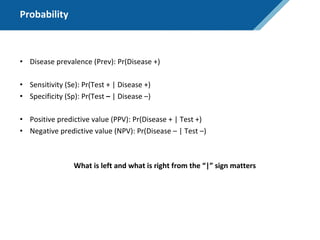
Here are the steps to solve this exercise: 1) Given: Prev = 30% Se = 99% Sp = 95% 2) Calculate other metrics: PPV = 75% NPV = 99.7% 3) Re-calculate NPV assuming Prev of 10%: NPV = 99.95% 4) Re-calculate NPV assuming Prev of 80%: NPV = 91.2% So in summary, the NPV decreases as the prevalence increases, since with a higher prevalence there is a higher chance that a negative test result represents a false negative.

1. Prediction modeling
Maarten van Smeden, Department of Clinical Epidemiology,
Leiden University Medical Center, Leiden, Netherlands
Berlin, Advanced Methods Methods in Health Data Sciences
Jan 16 2020

2. 2

3. 14-Jan-20Insert > Header & footer3

4. 4
Cartoon of Jim Borgman, first published by the Cincinnati Inquirer and King Features Syndicate April 27 1997

5. Cookbook review
5
Schoenfeld & Ioannidis, Am J Clin Nutr 2013, DOI: 10.3945/ajcn.112.047142
“We selected 50 common ingredients from random
recipes of a cookbook”

6. Cookbook review
veal, salt, pepper spice, flour, egg, bread, pork, butter, tomato,
lemon, duck, onion, celery, carrot, parsley, mace, sherry, olive,
mushroom, tripe, milk, cheese, coffee, bacon, sugar, lobster,
potato, beef, lamb, mustard, nuts, wine, peas, corn, cinnamon,
cayenne, orange, tea, rum, raisin, bay leaf, cloves, thyme, vanilla,
hickory, molasses, almonds, baking soda, ginger, terrapin
6
Schoenfeld & Ioannidis, Am J Clin Nutr 2013, DOI: 10.3945/ajcn.112.047142

7. Studies relating the ingredients to cancer: 40/50
veal, salt, pepper spice, flour, egg, bread, pork, butter, tomato,
lemon, duck, onion, celery, carrot, parsley, mace, sherry, olive,
mushroom, tripe, milk, cheese, coffee, bacon, sugar, lobster,
potato, beef, lamb, mustard, nuts, wine, peas, corn, cinnamon,
cayenne, orange, tea, rum, raisin, bay leaf, cloves, thyme, vanilla,
hickory, molasses, almonds, baking soda, ginger, terrapin
7
Schoenfeld & Ioannidis, Am J Clin Nutr 2013, DOI: 10.3945/ajcn.112.047142

8. Increased/decreased risk of developing cancer: 36/40
veal, salt, pepper spice, flour, egg, bread, pork, butter, tomato,
lemon, duck, onion, celery, carrot, parsley, mace, sherry, olive,
mushroom, tripe, milk, cheese, coffee, bacon, sugar, lobster,
potato, beef, lamb, mustard, nuts, wine, peas, corn, cinnamon,
cayenne, orange, tea, rum, raisin, bay leaf, cloves, thyme, vanilla,
hickory, molasses, almonds, baking soda, ginger, terrapin
8
Schoenfeld & Ioannidis, Am J Clin Nutr 2013, DOI: 10.3945/ajcn.112.047142

9. 9
Credits to Peter Tennant for identifying this example

11. To explain or to predict?
Explanatory models
• Theory: interest in regression coefficients
• Testing and comparing existing causal theories
• e.g. aetiology of illness, effect of treatment
Predictive models
• Interest in (risk) predictions of future observations
• No concern about causality
• Concerns about overfitting and optimism
• e.g. prognostic or diagnostic prediction model
Descriptive models
• Capture the data structure
11
Shmueli, Statistical Science 2010, DOI: 10.1214/10-STS330

12. To explain or to predict?
Explanatory models
• Theory: interest in regression coefficients
• Testing and comparing existing causal theories
• e.g. aetiology of illness, effect of treatment
Predictive models
• Interest in (risk) predictions of future observations
• No concern about causality
• Concerns about overfitting and optimism
• e.g. prognostic or diagnostic prediction model
Descriptive models
• Capture the data structure
12
A
L
Y
exposure outcome
confounder
Shmueli, Statistical Science 2010, DOI: 10.1214/10-STS330

13. Causal effect estimate
13
What would have happened with a group of individuals had they
received some treatment or exposure rather than another?

14. Image sources: https://bit.ly/3a9wRMj https://bit.ly/2uEDRQJ

15. Causal effect estimate
15
What would have happened with a group of individuals had they
received some treatment or exposure rather than another?

16. Randomized clinical trials
16
exchangeability

17. Randomized clinical trials
17
A
L
Y
exposure outcome
confounder

18. Observational (non-randomized) study
18
A
L
Y
exposure outcome
confounder

19. Observational study: diet -> diabetes, age
19
Age No diabetes Diabetes No diabetes Diabetes RR
< 50 years 19 1 37 3 1.50
≥ 50 years 28 12 12 8 1.33
Total 47 13 49 11 0.88
Traditional Exotic diet
50%
40%
30%
20%
10%
≥ 50 years
> 50 years
Total
Diabetes
risk
< 50 years
Numerical example adapted from Peter Tennant with permission: http://tiny.cc/ai6o8y

20. Observational study: diet -> diabetes, weight loss
20
Weight No diabetes Diabetes No diabetes Diabetes RR
Lost 19 1 37 3 1.50
Gained 28 12 12 8 1.33
Total 47 13 49 11 0.88
Traditional Exotic diet
50%
40%
30%
20%
10%
Gained wt
Lost wt
Total
Diabetes
risk
< 50 years
Numerical example adapted from Peter Tennant with permission: http://tiny.cc/ai6o8y

21. 12 RCTs; 52 nutritional epidemiology claims
0/52 replicated
5/52 effect in the opposite direction
21
Young & Karr, Significance, 2001, DOI: 10.1111/j.1740-9713.2011.00506.x

22. But…
22
Ellie Murray (Jul 13 2018): https://twitter.com/EpiEllie/status/1017622949799571456

23. 23

24. To explain or to predict?
Explanatory models
• Theory: interest in regression coefficients
• Testing and comparing existing causal theories
• e.g. aetiology of illness, effect of treatment
Predictive models
• Interest in (risk) predictions of future observations
• No concern about causality
• Concerns about overfitting and optimism
• e.g. prognostic or diagnostic prediction model
Descriptive models
• Capture the data structure
24
Shmueli, Statistical Science 2010, DOI: 10.1214/10-STS330

25. The “scientific value” of predictive modeling
25
1. Uncover potential new causal mechanisms and generation of new hypotheses
2. To discover and compare measures and operationalisations of constructs
3. Improving existing explanatory models by capturing underlying complex patterns
4. Reality check to theory: assessing distance between theory and practice
5. Compare competing theories by examining the predictive power
6. Generate knowledge of un-predictability
Shmueli, Statistical Science 2010, DOI: 10.1214/10-STS330 (p292)

26. Wells rule
26
Wells et al., Lancet, 1997. doi: 10.1016/S0140-6736(97)08140-3

27. Apgar
27
Apgar, JAMA, 1958. doi: 10.1001/jama.1958.03000150027007

28. 28
Courtesy, Anna Lohmann

29. 29
Courtesy, Anna Lohmann

30. Prediction
Usual aim: to make accurate predictions
… of a future outcome or presence of a disease
… for an individual patient
… generally based on >1 factor (predictor)
why?
• to inform decision making (about additional testing/treatment)
• for counseling
30

31. To explain or to predict?
Explanatory models
• Causality
• Understanding the role of elements in complex systems
• ”What will happen if….”
Predictive models
• Forecasting
• Often, focus is on the performance of the forecasting
• “What will happen ….”
Descriptive models
• “What happened?”
31
Require different
research design
and analysis
choices
• Confounding
• Stein’s paradox
• Estimators

32. Risk estimation example: SCORE
32
Conroy, European Heart Journal, 2003. doi: 10.1016/S0195-668X(03)00114-3

33. 33
https://apple.co/2s1aWWa

34. Risk prediction
Risk prediction can be broadly categorized into:
• Diagnostic: risk of a target disease being currently present vs not present
• Prognostic: risk of a certain health state over a certain time period
• Do we need a randomized controlled trial for diagnostic/prognostic prediction?
• Do we need counterfactual thinking?
34

35. Risk prediction
35
TRIPOD: Collins et al., Annals of Int Medicine, 2015. doi: 10.7326/M14-0697

36. Risk?
Risk = probability
36

37. Probability
37

38. 38

39. 39

40. How accurate is this point-of-care test?
40
image from: https://bit.ly/39LuajJ

41. Classical diagnostic test accuracy study
Patients suspected of target
condition
Reference standard for target
condition
Index test(s)
Domain
“Exposure”
“Outcome”

42. Classical diagnostic test accuracy study
Patients suspected of target
condition
Reference standard for target
condition
Index test(s)

43. Classical diagnostic test accuracy study
Patients suspected of target
condition
Reference standard for target
condition
Index test(s)
Role of time?
Cross-sectional in nature: index test and reference standard (in principle) at
same point in time to test for target condition at that time point

44. Classical diagnostic test accuracy study
Patients suspected of target
condition
Reference standard for target
condition
Index test(s)
Comparator for index test?
None, study of accuracy does not require a comparison to another index test

45. Classical diagnostic test accuracy study
Patients suspected of target
condition
Reference standard for target
condition
Index test(s)
Confounding (bias)?
No need for (conditional) exchangability to interpret accuracy. Confounding
(bias) is not an issue

46. Classical diagnostic test accuracy study
Prevalence = (A+B)/(A+B+C+D)
Sensitivity = A/(A+B)
Specificity = D/(C+D)
Positive predictive value = A/(A+C)
Negative predictive value = D/(B+D)

47. Probability
• Disease prevalence (Prev): Pr(Disease +)
• Sensitivity (Se): Pr(Test + | Disease +)
• Specificity (Sp): Pr(Test – | Disease –)
• Positive predictive value (PPV): Pr(Disease + | Test +)
• Negative predictive value (NPV): Pr(Disease – | Test –)
What is left and what is right from the “|” sign matters

48. All probabilities are conditional
• Some conditions are given without saying (e.g. probability is about human
individuals), others less so (e.g. prediction in first vs secondary care)
• Things that are constant (e.g. setting) do not enter in notation
• There is no such as thing as ”the probability”: context is everything

49. Small side step: the p-value
p-value*: Pr(Data|Hypothesis)
Is not: Pr(Hypothesis|Data)
Somewhat simplified, correct notation would be: Pr(T(X) ≥ x; hypothesis)

50. Small side step: the p-value
Pr(Death|Handgun)
= 5% to 20%*
Pr(Handgun|Death)
= 0.03%**
*from New York Times (http://www.nytimes.com article published: 2008/04/03/)
** from CBS StatLine (concerning deaths and registered gun crimes in 2015 in the Netherlands)

51. Bayes theorem
Pr(A|B) =
Pr B A ) Pr(A)
Pr(B)
Probability of A occurring given B happened
Probability of B occurring given A happened
Probability of A occurring
Probability of B occurring
Thomas Bayes
(1702-1761)

52. Bayesville
https://youtu.be/otdaJPVQIgg
https://youtu.be/otdaJPVQIgg

53. In-class exercise – ClearBlue compact pregnancy test
• Calculate Prev, Se, Sp, NPV and PPV
• Re-calculate NPV assuming Prev of 10%, and again with 80%
• Make use of NPV = Sp*(1-Prev)/[(1-Se)*Prev + Sp*(1-Prev)]

54. In reality
• Performance of the Clearblue COMPACT pregnancy test was worse: 38 additional
results among pregnant women were ‘non-conclusive’
• The reference standard was a ‘trained study coordinator’ reading of the same test

55. Diagnostic test is simplest prediction model
• Nowcasting (instead of forecasting)
• Best available prediction of target disease status is test result
• Assuming no other relevant information is available
• Risk prediction (probability) for disease:
• PPV with positive test
• 1-NPV with negative test

56. Model development

57. Research design: aims
Point of intended use of the risk model
• Primary care (paper/computer/app)?
• Secondary care (beside)?
• Low resource setting?
Complexity
• Number of predictors?
• Transparency of calculation?
• Should it be fast?

58. Research design: design of data collection
Prospective cohort study: measurement of predictors at baseline + follow-up until event
occurs (time-horizon)
Alternatives
• Randomized trials?
• Routine care data?
• Case-control?

59. Statistical models
• Regression models for binary/time-to-event outcomes
• Logistic regression
• Cox proportional hazards models (or parametric alternatives)
• Alternatives
• Multinomial and ordinal models
• Decision trees (and decendants)
• Neural networks

60. Regression model specification
f(X): linear predictor (lp)
lp = b0 + b1X1 + … + bPXP (only "main effects")
Logistic regression: Pr(Y = 1 | X1 ,…,XP ) = 1/(1 + exp{-lp})
b0; intercept, important?

61. Intercept
Intercept = 0 - c, intercept = 0, intercept = 0 + c

62. Model predictive performance

63. Discrimination
• Sensitivity/specificity trade-off
• Arbitrary choice threshold ! Many
possible sensitivity/specificity pairs
• All pairs in 1 graph: ROC curve
• Area under the ROC-curve:
probability that a random individual
with event has a higher predicted
probability than a random individual
without event
• Area under the ROC-curve: the c- statistic (for logistic regression) takes
on values between 0.5 (no better than a coin-ip) and 1.0 (perfect
discrimination)

64. Calibration
https://bmcmedicine.biomedcentral.com/articles/10.1186/s12916-019-1466-7

65. Optimism
Predictive performance evaluations are too optimistic when estimated on the same data
where the risk prediction model was developed. This is therefore called apparent
performance of the model
Optimism can be large, especially in small datasets and with a large number of predictors
To get a better estimate of the predictive performance (more about this next week):
• Internal validation (same data sample)
• External validation (other data sample)

66. https://twitter.com/LesGuessing/status/997146590442799105

67. 1955: Stein’s paradox

68. Stein’s paradox in words (rather simplified)
When one has three or more units (say, individuals), and for each unit one can calculate
an average score (say, average blood pressure), then the best guess of future
observations for each unit (say, blood pressure tomorrow) is NOT the average score.

69. 1961: James-Stein estimator: the next Symposium
James and Stein. Estimation with quadratic loss. Proceedings of the fourth Berkeley symposium on
mathematical statistics and probability. Vol. 1. 1961.

70. 1977

71. 1977: Baseball example
Squared error reduced from .077 to .022

72. Stein’s paradox
• Probably among the most surprising (and initially doubted) phenomena in statistics
• Now a large “family”: shrinkage estimators reduce prediction variance to an extent
that typically outweighs the bias that is introduced
• Bias/variance trade-off principle has motivated many statistical and machine learning
developments
Expected prediction error = irreducible error + bias2 + variance

83. Simulate 100 times

84. Not just lucky
• 5% reduction in MSPE just by shrinkage estimator
• Van Houwelingen and le Cessie’s heuristic shrinkage factor

85. Heuristic argument for shrinkage

86. Heuristic argument for shrinkage

87. Overfitting
"Idiosyncrasies in the data are fitted rather than generalizable patterns. A
model may hence not be applicable to new patients, even when the setting of
application is very similar to the development setting."
Steyerberg (2009). Clinical Prediction Models.

88. Overfitting versus underfitting

89. To avoid overfitting…
Large data (sample size / no. events) and to pre-specify your analyses as much as
possible!
And:
• Be conservative when removing predictor variables
• Apply shrinkage methods
• Correct for optimism

90. EPV – rule of thumb
Events per variable (EPV) for logistic/survival models:
number of events (smallest outcome group)
number of candidate predictor variables1
EPV = 10 commonly used minimal criterion

91. EPV – rule of dumb?
• EPV values for reliable selection of predictors from a larger set of
candidate predictors may be as large as 50
• Statistical simulation studies on the minimal EPV rules are highly
heterogeneous and have large problems

92. New sample size proposals

93. Variable selection
• Selection unstable
• Selection and order of entry often overinterpreted
• Limited power to detect true effects
• Predictive ability suffers, ‘underfitting’
• Risk of false-positive associations
• Multiple testing, ‘overfitting’
• Inference biased
• P-values exaggerated; standard errors too small
• Estimated coefficients biased
• ‘testimation’

94. Selection with small sample size

95. Conditional probabilities are at the core of prediction
• Perfect or near-perfect predicting models?
Suspect!
• Proving that a probability model generates a wrong risk prediction?
Difficult!

96. When is a risk model ready for use?

97. Prediction model landscape
>110 models for prostate cancer (Shariat 2008)
>100 models for Traumatic Brain Injury (Perel 2006)
83 models for stroke (Counsell 2001)
54 models for breast cancer (Altman 2009)
43 models for type 2 diabetes (Collins 2011; Dieren 2012)
31 models for osteoporotic fracture (Steurer 2011)
29 models in reproductive medicine (Leushuis 2009)
26 models for hospital readmission (Kansagara 2011)
>25 models for length of stay in cardiac surgery (Ettema 2010)
>350 models for CVD outcomes (Damen 2016)
• Few prediction models are externally validated
• Predictive performance often poor
97

98. To explain or to predict?
Explanatory models
• Theory: interest in regression coefficients
• Testing and comparing existing causal theories
• e.g. aetiology of illness, effect of treatment
Predictive models
• Interest in (risk) predictions of future observations
• No concern about causality
• Concerns about overfitting and optimism
• e.g. prognostic or diagnostic prediction model
Descriptive models
• Capture the data structure
98
Shmueli, Statistical Science 2010, DOI: 10.1214/10-STS330

99. Problems in common (selection)
• Generalizability/transportability
• Missing values
• Model misspecification
• Measurement and misclassification error
99

100. 100

101. Two hour tutorial to R (free): www.r-tutorial.nl
Repository of open datasets: http://mvansmeden.com/post/opendatarepos/
101