Data analytics concepts

Data analytics Concepts
UCSC - 2013
Hiranthi Tennakoon
Feature Selection Algorithms
SOM training
Using SOM in practical scenario

Part 1
 Introduction to Branch And Bound
 Analysis the Algorithm
 Demonstrate Branch And Bound Algorithm
 Applications
 Observation and recommendation of algorithm
 Introduction to Beam search algorithm
 Analysis the Algorithm
 Demonstrate Beam search algorithm
 Applications
 Observation and recommendation of algorithm

Part 2
 Install MATLAB toolkit
 Train data set to SOM
Part 3
 Introduction to SOM algorithm
 Using SOM to solve traveling salesman problem

 When try to learn a data set, it is necessary of identify
features of the dataset given.
 For a particular n number of features, performance of
the criteria function is increased and if we add more
features again and again, the performance of the
criterion function would be decreased which is called
“Curse of dimensionality”

 Curse of dimensionality means when increase number of
dimensions in criterion function, it’s performance decreases
because of the miss classification of classes in dataset
 This occurs due to the reduction of density in solution
space
 In order to overcome this situation we have to either
increase the data set, or reduce the number of features for
classification
 We need “Feature selection” to select optimum subset of
features

 Branch and Bound algorithm was developed by Narendra
and Fukunaga in 1977
 Guaranteed to find the optimal feature subset without
evaluating all possible subsets
 Branch & Bound is an exponential search method
 Assumes that feature selection criterion is monotonic

What is monotonicity property?
 It ensures that the values of the leaf nodes of that branch
cannot be better than it’s parent node
 X,Y are feature subsets of given set.
 This property reduces the number of nodes and branches
of the search tree that have to be explored
X ⊂ Y => J(X) < J(Y)
Ex: Y = {a,b,c}
X = {b,c}

 Basic concept – Divide and conquer
 Branch – Partition full set of features into smaller subsets
 Bound – Provide a bound for the best solution in the subset
where it discard if bound points out that it can’t contain an
optimal solution
 Start with all n features in the root
 For each tree level, a limited number of sub-trees is
generated by deleting one feature from the set of features
from the parent node

Step 1 - Construct an ordered tree by
satisfying the Monotonicity property
Step 2 - Traverse the tree from right to left in
depth first search pattern
Step 3 - Pruning

Construct an ordered tree by satisfying the Monotonicity
property
 If Y is the full set of features, it obtains the Y’ optimal feature
subset by removing j features y1, y2,y3..yj from the subset.
 The monotonicity condition assumes that, for feature subsets
y1 , y2 … yj where,
y1 ⊂ y2 ⊂ y3 …. ⊂ yj
The criterion function J fulfills,
J(y1) < J(y2) < J(y3) < … < J(yj)

 Root of the tree is the set of all n features and leaves are
target m subsets of features
 For each tree level, a limited number of sub-trees is
generated by deleting one feature from the set of features
from the parent node
{ Y1,Y2,Y3 }
{ Y2,Y3 } { Y1,Y3 } { Y1,Y2 }
Y1 Y2 Y3
All features
(n)
Target subset
(m)
Removed
feature

 Number of leaf nodes in tree = nCm
 Number of levels = n – m
 No of leaf nodes = 3C2 = 3
 No of levels = 3 – 2 = 1
{ Y1,Y2,Y3
}
{ Y2,Y3
}
{ Y1,Y3
}
{ Y1,Y2
}
Y
1
Y
2
Y
3

 Traverse the tree from right to left in depth first search
pattern
 If the value of the criterion is less than the boundary
value at a given node,
All its child nodes will also have a value less than
criterion value according to the monotonicity property.

 When the criterion value J(Ym) of some internal node is
lower than the current bound, due to the Monotonicity
condition the whole sub tree may be cut off and many
computations may be omitted
 Branch and Bound creates tree with all possible
combinations of s element subsets from the n whole
set, but searches only some of them

Find the best 3 features from 6 full set of features
1,2,3,4,5,6
? ? ?

 No of levels = 6-3 = 3 (6  5  4  3)
 No of leaf nodes = 6C3 = 20
 Choose a criterion function J(x).

1,2,3,4,5,6
2,3,4,5,6 1,3,4,5,6 1,2,4,5,6
32
1
1,2,3,5,6
4

1,2,3,4,5,6
2,3,4,5,6 1,3,4,5,6 1,2,4,5,6
32
1
1,2,3,5,6
4
3,4,
5,6
2,4,5
,6
2,3,5
,6
1,4,
5,6
1,3,
5,6
1,3,
4,6
2
3 4 3 4
2,3,4
,6
5 5
1,2,
5,6
4 5
1,2,
4,6
1,2,
3,6
6

1,2,3,4,5,6
2,3,4,5,6 1,3,4,5,6 1,2,4,5,6
32
1
1,2,3,5,6
4
3,4,
5,6
2,4,5
,6
2,3,5
,6
1,4,
5,6
1,3,
5,6
1,3,
4,6
2
3 4 3 4
2,3,4
,6
5 5
1,2,
5,6
4 5
1,2,
4,6
1,2,
3,6
5
1,3,
6
1,3
,4,
1,2,
6
1,2,
4
1,
2,
3
5 6 5 6 6
1,2,
5
6
1,3,
5
6

88
62 59 65
32
1
60
4
29 50 55 51 32 49
2
3 4 3 4
44
5 5
62
4 5
55 40
5
21 31 25 30 27
5 6 5 6 6
38
6
33
6
Bound
value
Assume these are the
values from criterion
function

88
62 59 65
32
1
60
4
29 50 55 51 32 49
2
3 4 3 4
44
5 5
62
4 5
55 40
5
21 31 25 30 27
5 6 5 6 6
38
6
33
6
Update
Bound
value

88
62 59 65
32
1
60
4
29 50 55 51 32 49
2
3 4 3 4
44
5 5
62
4 5
55 40
5
21 31 25 30 27
5 6 5 6 6
38
6
33
6
Bound
value
X
XXXXXXX
Current Node value < Bound node ;
Prune the below branches
Bound – 38 , Features {1,2,5}

A branch and bound algorithm for scheduling trains in a
railway network
 The paper studies a train scheduling problem faced by railway
infrastructure managers during real-time traffic control
 When train operations are delayed or stopped, a new conflict-
free timetable of feasible arrival and departure times needs to
be re-computed, such that the deviation from the original one
is minimized
 They have develop a branch and bound algorithm which
includes implication rules enabling to speed up the
computation
Branch And Bound Applications

 Train connection graph of EMU circulation scheduling model is
constructed
 Through the analyzing of the features of the structure of the
feasible EMU circulation plan, they have designed an exact
branch and bound algorithm for solving the problem
 Put the initial problem down to a graph designing problem
 A branch strategy is proposed to cope with the maintenance
constraints and to generate an optimal circulation plan

 Comparison of the proposed branch and bound method with
the heuristics - The running time needed by branch and bound
method is more reasonable when dealing with the instance of
the problem

A Lagrangian-Based Branch And Bound Algorithm for the
Two Level Uncapacitated Facility Location
Problem(TUFLP) with Single-Assignment Constraints
 Two-Level uncapacitated facility location problem with single
assignment constraints problem that arises in industrial applications
in freight transportation and telecommunications
 Finite potential facility locations Upper level Depots +
Lower
Level satellites
Problem – Which depots and satellite to open
Which depot-satellite pair each customer should be
assigned
Replace

 Every B & B algorithm requires large computations
- Not only the target subsets of r features, but also their
supersets have to be evaluated
 Criterion function would be computed in every tree node -
Same as the Exhaustive search
 Criterion value computation is usually slower near to the root
- Evaluated feature subsets are larger J(Y1,Y2…Yn)
 Sub tree cut-offs are less frequent near to the root
-Higher criterion values following from larger subsets are
compared to the bound, which is updated in leaves
Observations and recommendations

 The B & B algorithm usually spends most of the time by
tedious,
less promising evaluation of the tree nodes in levels closer to
the
root
 This effect is to be expected, especially for r <<< n
Observations and recommendations

 Beam Search was developed in an attempt to achieve the
optimal solution found by the Breadth-First Search Algorithm
without consuming too much memory
 Beam search uses Breadth-First Search strategy to expand
nodes in the tree
 Beam width (B) is given prior in the algorithm which is the
specific number of nodes that are stored at each level
 In breath first search, the best promising nodes with high
values are carry forward to next level and others are discarded
(Pruned)
Introduction

Step 1- Calculate the performance of each individual feature
using criterion function
Step 2 - Select beam width B
Step 3 - Start with no features
Step 4 - Only best B subsets are carried to the next level
Step 5 - Add new best promising features to the selected
features except the original features that has been already
selected
Step 6 - Repeat the process until the tree reach to the target
subset
Analysis

Find the best 3 features from 6 full set of features
Analysis - Example
1,2,3,4,5,6
? ? ?

1 2 3 4
5
Example
{ }
2530 14 28 16 25
6
{1} {2} {3} {4} {5} {6}
Start with no features and calculate the values of
each individual feature, Find the best performing
feature from the set

1 2 3 4
5
Example
{ }
4
5
30 32 29 21 29
6
{1} {2} {3} {4} {5} {6}
Start with no features and calculate the values of each
individual feature, Find the best performing feature from the
set.
B = 3

1 2 3 4
5
Example
{ }
4
5
30 32 29 21
{1,2} {2,4} {5,6}
Select the next B set of best promising nodes and forward to
next step, Prune less performing nodes
B = 3
64 43 52 39 31 35 60 39
2 3 4 5 6 1 3 4 5 6 1 2 3 4 6
19
41 56 34 35 34 48 67

1 2 3 4 5 6
Example
{ }
4
5
30 32 29 21
{5,6,2}
Highest criterion value for three feature set
Best feature {5,6,2}
B = 3
64 43 52 39 37 35 60 39
2 3 4 5 6 1 3 4 5 6 1 2 3 4 6
19
41 56 52 47 55 48 67
73 62 70 65 62 88 94 82 6969 88 72
3 4 5 6 1 3 5 6 1
2 3
4

Job shop scheduling with beam search
 The job shop problem is to determine the start and completion
time of operations of a set of jobs on a set of machines,
subject to the constraint that each machine can handle at most
one job at a time (capacity constraints) and each job has a
specified processing order through the machines
 Finite set J of jobs
 Finite set M of machines
 For each job j 2 J, a permutation (rj 1; . . . ; rj m) of the
machines (where m ˆjMj) represents the processing order of
job j through the machines
Applications

 They have used beam search algorithm to solve this job shop
scheduling problem
 They have come up with two issues when using beam search
algorithm ;
1. Search tree representation
2. Ditermination of a search methodology
 So they have used Baker’s two search tree generation
procedures (active and non delay) to generate branches from
a given node
 In order to address the second issue, all the nodes at level 1
are globally evaluated to determine the best ß number of
promising nodes.
Applications

 There is no backtracking - The intent of this technique is to
search quickly
 Therefore, beam search methods are not guaranteed to find
an optimal solution and cannot recover from wrong decisions
 Duplications cannot be avoided in the tree
 If a node leading to the optimal solution is discarded during the
search process, there is no way to reach that optimal solution
afterwards
 Beam width parameter K is fixed to a value before searching
starts
 A wider beam width allows greater safety, but it will increase
the computational cost
Observations and Recommendations

Part II
Q1 : Train a SOM algorithm for the given data sets and obtain the possible clusters
maps with the corresponding class labels
Q2 : Draw the confusion matrix for the dataset

Tools used
 MATLAB R2013a
 kohonen_cpann_toolbox_3.8
 Provided dataset
Q1

STEP 1
 Install MATLAB R2013a
 Import library toolkit
 Set path  Set path to imported library toolkit folder
Q1

STEP 2
 Open the downloaded data set and replace the class
names as follows
 C1 1
 C2  2
 C3  3
 C4  4
 Save the modified data file inside the toolkit folder
(mydata.csv)
Q1

STEP 3
 Open MATLAB and open a new script in MATLAB
 Write the following code in new script
 Save file as script.m
 Execute command “script” in MATLAB console
Q1

STEP 4
 Execute command “model_gui” in console, it will open
following window
 File  Load data  Select X data and load
Q1

 File  Select class  select t and load
Q1

STEP 5
 Then calculate the model in following window
Q1

STEP 6
 Setup the following settings and click calculate model
Q1

 Click on view top map button to get the topology with Class
label
Q1

Top map for class 1 with class labels
Q1

Q1

Q2 – Confusion Matrix for the data set

 Developed by Teuvo Kohonen in 1980s
 There are two layers, Input and Output which are completely
connected
 Output neurons are interconnected within a defined
neighborhood relation (topology) which is decreasing gradually
Introduction to SOM

How SOM is differed from ANN?
 In ANN it has weighted connections, SOM connections are not
weighted
 ANN have more than two layers, it has middle layers, SOM is
having only two layers ; Input and output
 ANN back propagation is done which is not done in SOM
Introduction to SOM

 Weight of each node is initiated
 The input vector is chosen at random from the set of training
data
 The features of the randomly selected input node is matched
with the each node in output layer
SOM Algorithm

 Calculate the weight of each node and identify the winning
node which is having the minimum weight different with input
vector
 Calculate the radius of neighborhood and learning rate –
Which is diminishing over iterations
 Neighborhood nodes’ weight are adjusted to make them more
like the input node.
 Continue this process until no change in the feature map
SOM Algorithm

What is Traveling salesmen problem?
 Salesman is given a list of cities and their pair wise distances,
the task is to find a shortest possible tour that visits each city
exactly once in their sales tours
 Have to find the optimal routes of delivery or collection from
one or several depots to a number of cities or customers
SOM Algorithm To solve TSP problem

 A two‐layer network - A two‐dimensional input and m
output neurons
 Two dimensional input
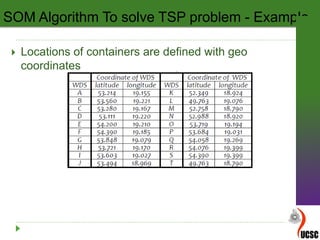
- defines the coordinates of the waste disposal sites (WDS) in
the two dimensional Euclidian space
- are fully connected to every output neuron
 To get the scaled coordinates for WDS, range [0‐1] was
performed using the equation
SOM Algorithm To solve TSP problem - Steps

 SOM architecture consists of a one ring which can
be considered as a route for an ideal problem

 What is called the weight of a neuron in SOM?
- Define the position of the neuron in the ring
- Initially all m neurons in the ring are equally positioned on a
circle
- Circle radius – I
- Angle position of given neuron - 360º/m
 Randomly select input data and presented to the SOM
 The winner neuron is the neuron I* with the minimum distance
to the presenting city
 Same as SOM the winner neuron and neighboring neurons
are moving toward the presented i‐th input neuron

 Neighborhood function
 Weight update function
 α - learning rate
 σ - neighborhood function variance
 Both are set to large value at the beginning and diminishing
over time

 Finally after many iterations
- The neurons tend to move closer to the WDS input vector
- Then output neurons are attached in WDS
 After all the neurons in output layer are attached in the WDS,
simply walk around the neurons connections and read the
WDS coordinates in the order that they appear
 Resulting sequence is the TSP solution

 In order to solve the TSP problem, 1-D network has
to be maintained
 Number of neurons = Number of cities
 1 to 1 mapping between neurons and cities
 All the neurons are organized in a vector which
represents sequence of cities that must be visited
SOM Algorithm To solve TSP problem – STEPS

Apply SOM to solve the problem of 20 waste disposal
sites
JKP company has a large transport costs for emptying the
plastic waste containers due to lack of optimal route of
the vehicle. They need to find the optimal route for vehicle to
collect plastic waste containers
Restrictions
 You must visit each city only once
 You must return to the original starting point
SOM Algorithm To solve TSP problem - Example

 Locations of containers are defined with geo
coordinates

Have done three simulations to find the solution
1 - Performed with 1000 epochs and the learning rate 0.1. This
corresponds to the first phase in which neurons tend to WDC

2 - Performed with 2000 epochs and the learning rate 0.1
- All the neurons are closer to WDC
- Some are in the centers of these coordinates
3 - corresponds to the maximum number of epochs.
 All m neurons coincided with WDC.
 The route can be read from the weighting coefficients of
neurons
 Optimum vehicle route is

Advantages
 Easy implementation and fast computation,
 robust applicability
 production of good solutions.
 SOM provides flexible and quick means to obtain optimized
routs for collecting plastic waste
Disadvantages
 Some of the SOM parameters need to be optimized such as
learning rate, neighborhood distance and number of iterations.

[1]"A Branch and Bound Algorithm for the Exact Solution of the Problem of
EMU Circulation Scheduling in Railway Network", Hindawi, 2015.
[2]"Beam-ACO—hybridizing ant colony optimization with beam search: an
application to open shop scheduling", ELSEVIER, 2017.
[3]"Kohonen Self-Organizing Map for the Traveling Salesperson Problem",
2017.
References

Data analytics concepts

More Related Content

What's hot

Similar to Data analytics concepts

Recently uploaded

Data analytics concepts