Synthetic Curves.pdf

Chapter 4 - Curves
CHAPTER 4
CURVES
4.1 Introduction
In order to understand the significance of curves, we should look into the types of model
representations that are used in geometric modeling. Curves play a very significant role in CAD
modeling, especially, for generating a wireframe model, which is the simplest form for
representing a model.
We can display an object on a monitor screen in three different computer-model forms:
• Wireframe model
• Surface Model
• Solid model
Wireframe model: A wireframe model consist of points and curves only, and looks as if its
made up with a bunch of wires. This is the simplest CAD model of an object. Advantages of this
type of model include ease of creation and low level hardware and software requirements.
Additionally, the data storage requirement is low. The main disadvantage of a wireframe model
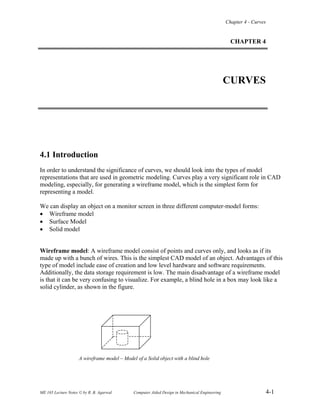
is that it can be very confusing to visualize. For example, a blind hole in a box may look like a
solid cylinder, as shown in the figure.
A wireframe model – Model of a Solid object with a blind hole
ME 165 Lecture Notes © by R. B. Agarwal Computer Aided Design in Mechanical Engineering 4-1

Chapter 4 - Curves
In spite of its ambiguity, a wireframe model is still the most preferred form, because it can be
created quickly and easily to verify a concept of an object. The wireframe model creation is
somewhat similar to drawing a sketch by hand to communicate or conceptualize an object. As
stated earlier, a wireframe model is created using points and curves only.
Surface Model: sweeping a curve around or along an axis can create a surface model. The
figures below show two instances of generating a surface model.
Generating a cylinder by sweeping a circle generating a donut by sweeping a circle
in the direction of an axis around an axis
The appearance or resolution of a surface model depends on the number of sweeping instances
we select. For a realistic looking model, we need to select a large number of instances, requiring
a large computer memory, or, opt for a not-so realistic model by selecting a small number of
instances, and save memory. In some commercial CAD packages we have the option of selecting
the resolution of a model, other packages have a fixed value for resolution that cannot be
changed by users.
Surface models are useful for representing surfaces such as a soft-drink bottle, automobile
fender, aircraft wing, and in general, any complicated curved surface. One of the limitations of a
surface model is that there is no geometric definition of points that lie inside or outside the
surface.
Solid Model: Representation of an object by a solid model is
relatively a new concept. There were only a couple of solids
modeling CAD programs available in late 1980s, and they
required mainframe computers to run on. However, in 1990s,
due to the low cost and high speed, PCs have become the
most popular solid modeling software platform, prompting
almost all the CAD vendors to introduce their 3-D solid
modeling software that will run on a PC.
Solid models represent objects in a very realistic and
unambiguous form; however, they require a large amount of
storage memory and high-end computer hardware. A solid
model can be shaded and rendered in desired colors to give it a more realist appearance.

Chapter 4 - Curves
4.2 Role of Curves in Geometric Modeling
Curves are used to draw a wireframe model, which consists of points and curves; the curves are
utilized to generate surfaces by performing parametric transformations on them. A curve can be
as simple as a line or as complex as a B-spline. In general, curves can be classified as follows:
• Analytical Curves: This type of curve can be represented by a simple mathematical
equation, such as, a circle or an ellipse. They have a fixed form and cannot be modified to
achieve a shape that violates the mathematical equations.
• Interpolated curves: An interpolated curve is drawn by interpolating the given data points
and has a fixed form, dictated by the given data points. These curves have some limited
flexibility in shape creation, dictated by the data points.
• Approximated Curves: These curves provide the most flexibility in drawing curves of very
complex shapes. The model of a curved automobile fender can be easily created with the help
of approximated curves and surfaces.
In general, sweeping a curve along or around an axis creates a surface, and the generated surface
will be of the same type as the generating curve, e.g., a fixed form curve will generate a fixed
form surface.
As stated earlier, curves are used to generate surfaces. To facilitate the computer-language
algorithm, curves are represented by parametric equations. Non-parametric equations are used
only to locate a point of intersection on the curve, and not for generating them. Let us briefly
discus the parametric and non-parametric form of a curve.

Chapter 4 - Curves
4.3 Parametric and Non-parametric Equations of a Curve
The mathematical representation of a curve can be classified as either parametric or non-
parametric (natural). A non-parametric equation has the form,
y = c1 + c2 x + c3 x2
+ c4 x3
Explicit non-parametric equation
This is an example of an explicit non-parametric curve form. In this equation, there is a unique
single value of the dependent variable for each value of the independent variable. The implicit
non-parametric form of an equation is,
(x – xc)2
+ (y – yc)2
= r2
Implicit non-parametric equation
In this equation, no distinction is made between the dependent and the independent variables.
Parametric Equations: Parametric equations describe the dependent and independent variables
in terms of a parameter. The equation can be converted to a non-parametric form, by eliminating
the dependent and independent variables from the equation. Parametric equations allow great
versatility in constructing space curves that are multi-valued and easily manipulated. Parametric
curves can be defined in a constrained period (0 ≤ t ≤ 1); since curves are usually bounded in
computer graphics, this characteristic is of considerable importance. Therefore, parametric form
is the most common form of curve representation in geometric modeling. Examples of
parametric and non-parametric equations follow.
Non-Parametric Parametric
Circle: x2
+ y2
= r2
x = r cosθ, y = r sinθ
Where, θ is the parameter.
CAD programs prefer a parametric equation for generating a curve. Parametric equations are
converted into matrix equations – to facilitate a computer solution, and then varying a parameter
from 0 to 1 creates the points or curves. In this course, we will use the following parameters,
with the range indicated,
0 ≤ t ≤ 1 0 ≤ s ≤ 1 0 ≤ θ ≤ 2πs 0 ≤ ϕ ≤ 2πs

Chapter 4 - Curves
4.4 Fixed-Form or Analytical Curves
4.4.1 Equation of a Straight Line: The simplest fixed-form curve is a straight line.
Parametric equation of a straight line is given as,
P(t) = A + (B-A) t (4.1)
The parametric equation of line AB can be derived as,
B (x2, y2)
x = x1 + (x2 - x1) t
y = y1 + (y2 - y1) t
. P (x, y)
where, 0 ≤ t ≤ 1
A (x1, y1)
The point P on the line is sweeped from A to B,
as the value of t is varied from 0 to 1.
4.4.2 Conic Sections or Conic Curves
A conic curve is generated when a plane intersects a cone, as shown.
B
P Q
A A

Chapter 4 - Curves
The intersection of the plane PQ and the cone is a circle, where as, the intersection created by the
plane AB is an ellipse. Other curves that can be created are parabola and hyperbola.
Conic curves are used to create simple wireframe models of objects, which have edges that can
be represented by these analytical curves. The fixed-form or analytical curves do not have
inflection points, i.e., curves have slopes that are either positive or negative and do not change
their sign (positive slope will remain positive and negative slope will remain negative). All conic
curves can be represented by a quadratic equation, for example, circular and elliptical curves
have quadratic polynomial equations.
4.4.3 Circular Curve
The non-parametric equation of a circle is,
(x – xc)2
+ (y – yc)2
= r2
(4.2)
Where, xc, and yc are coordinates of the center, and r is radius of the circle.
If we were to use this form of the equation for plotting a circle or a circular curve, we will first
calculate several values of x and y along the circumference of the circle, and then plot them. The
curve thus generated will be of a poor quality, unless we plot a very large number of data points,
which will result in a significant demand for storage of these data points. Therefore, as stated
earlier, in CAD programs, we use a parametric equation, which avoids the need for storage of the
data points, and provides a smooth curve. The parametric equation of the above circle can be
written as,
xi = xc + r cosθ
yi = yc + r sinθ (4.3)
This equation is converted into a matrix form so that a computer can solve it. We will now
convert this equation into a matrix form.
Let us assume that the plot starts at the point (xi, yi), and the center lies at the origin. We
increment θ to (θ +∆θ), giving us the new point on the circle (xi+1, yi+1), or
xi+1 = r cos(θ +∆θ)
yi+1 = r sin(θ +∆θ)

Chapter 4 - Curves
(xi+1, yi+1)
∇θ (xi, yi)
θ
Expanding it by the use of
trigonometric identities, we get:
xi+1 = r cosθ cos∆θ - r sinθ sin∆θ
yi+1 = r sinθ cos∆θ + r cosθ sin∆θ
Substituting the values: xi = r cosθ, and yi = r sinθ, we get
xi+1 = xi cos∆θ - yi sin∆θ
yi+1 = yi cos∆θ + xi sin∆θ
In matrix form, these equations can be written as,
cos∆θ sin∆θ 0 0
[xi+1 yi+1 0 1] = [xi yi 0 1] - sin∆θ cos∆θ 0 0 (4.4)
0 0 1 0
0 0 0 1
Equation (4.4) is valid for a circle that has center at the origin. To find the equation of a circle
that has center located at an arbitrary point (xc, yc), we can use the translation transformation.
Note that the equation (4.4) can be interpreted as rotational transformation of points xi and yi
about the origin. Now, instead of rotation about the origin, we wish to rotate the point about the
fixed point (xc, yc). This can be accomplished by the three-step approach, discussed in chapter 2,
i.e., first translate the fixed point to the origin, rotate the object, and finally translate it so that the
fixed point is restored to its original position. Using this procedure we will get:

Chapter 4 - Curves
[xi+1 yi+1 0 1] =
1 0 0 0 cos∆θ sin∆θ 0 0
[xi yi 0 1] 0 1 0 0 - sin∆θ cos∆θ 0 0
0 0 1 0 0 0 1 0
-xc -yc 0 1 0 0 0 1
1 0 0 0
0 1 0 0 (4.5)
0 0 1 0
xc yc 0 1
Simplifying the equation we get,
xi+1 = xc + (xi – xc) cos∆θ - (yi – yc) sin∆θ
yi+1 = yc + (xi – xc) sin∆θ + (yi – yc) cos∆θ (4.6)
Even though, equations (4.6) can be used as an iterative formula to plot a circle or a circular
curve, using the EXCEL or MATLAB, or any other plot routines, the matrix equation (4.5) is the
preferred form for a CAD program. The original CAD programs used iterative formulas to
generate curves. The BASIC and FORTRAN languages were used to write the CAD codes.

Chapter 4 - Curves
4.4.4 Ellipse
Following the procedure outlined in the previous section, we can derive the parametric equations
of an ellipse. Parametric equation of an ellipse is given by
the equation
xi = a cosθ
yi = b sinθ
2b
For a point on the ellipse, in general, the equation is
xi+1 = xi cos∆θ – (a/b) yi sin∆θ 2a
yi+1 = yi cos∆θ – (b/a) xi sin∆θ (4.7)
For a more general case, when the axes of the ellipse are not parallel to the coordinate axes, and
the center of the ellipse is at a distance xc, yc from the origin, the equation of the ellipse is given
below. Let α be the angle that the major axis makes with the horizontal (x-axis), as shown. The
equation of the ellipse can be derived as
xi = xc + x’i cosα – y’i sinα
yi = yc + x’i sinα + y’i cosα (4.8)
Where, x’ and y’ are the coordinate values of a
Point on the ellipse, in term of the rotated axes
x’ and y’.
Equations (4.8) can be used to write either as an
iterative formula or as a matrix equation for creating
an elliptical curve.

Chapter 4 - Curves
4.5 Interpolated Curves
Interpolation method can be applied to draw curves that pass through a set of the given data
points. The resulting curve can be a straight line, quadratic, cubic, or higher order curve. We are
quite familiar, and have used, the linear interpolation of a straight line, given by the formula
f(x) = f(xi) + [f(xi+1) – f(xi)] [(x-xi) / (xi+1 – xi)] (4.9)
Now, we will discuss the higher order curves, which are represented by higher order
polynomials. Lagrange polynomial is a popular polynomial function used for interpolation of
high order polynomials.
4.5.1 Lagrange Polynomial
When a sequence of planar points (x0, y0), (x1, y1), (x2, y2), ….(xn, yn) is given, the nth
degree of
interpolated polynomial can be calculated by the Lagrange Polynomial equation,
fn (x) = Σ yi Li,n (x) (4.10)
where,
Li,n (x) = [(x –x0)…. (x –xi-1) (x –xi+1)…. (x –xn)] / [(xi –x0)…. (xi –xi-1) (xi –xi+1)…. (xi –xn)]
To understand the above expression better, note that
• The term (x –xi) is skipped in the numerator, and
• The denominator starts with the term (xi –x0) and skips the term (xi –xi), which will make the
expression equal to infinity.
Example: Using the Lagrange polynomial, find the expression of the curve containing the
points, P0(1, 1), P1(2, 2), P2(3, 1)
Solution: Here, n = 2 and x0 =1, y0 = 1, x1 = 2, y1 = 2, etc. The polynomial is of a second
degree. Expanding the Lagrange equation, we get,
f2 (x) = y0 [(x - x1) (x - x2)] / [(x0 – x1) (x0 – x2)] + y1 [(x – x0) (x - x2)] /
[(x1 – x0) (x1 – x2)] + y2 [(x – x0) (x – x1)] / [(x2 – x0) (x2 – x1)]

Chapter 4 - Curves
= (1) [(x – 2) (x – 3)] / [(1 – 2) (1 – 3)] + (2) [(x-1) (x – 3)] / [(2 – 1) (2 – 3)] +
(1) [(x – 1) (x - 2)] / [(3 – 1) (3- 2)]
= ½ (x2
– 5x + 6) – 2 (x2
– 4 x + 3) + ½ (x2
– 3 x + 2) or
f2 (x) = - x2
+ 4 x – 2
This is the explicit non-parametric equation of a circle; the given points lie on the circumference.
4.5.2 Parametric Cubic Curve or Cubic Spline – Synthetic Curves
The analytical and interpolated curves, discussed in the previous section (4.4) and (4.5) are
insufficient to meet the requirements of mechanical parts that have complex curved shapes, such
as, propeller blades, aircraft fuselage, automobile body, etc. These components contain non-
analytical, synthetic curves. Design of curved boundaries and surfaces require curve
representations that can be manipulated by changing data points, which will create bends and
sharp turns in the shape of the curve. The curves are called synthetic curves, and the data points
are called vertices or control points. If the curve passes through all the data points, it is called an
interpolant (interpolated). Smoothness of the curve is the most important requirement of a
synthetic curve.
Various continuity requirements at the data points can be specified to impose various degrees of
smoothness of the curve. A complex curve may consist of several curve segments joined
together. Smoothness of the resulting curve is assured by imposing one of the continuity
requirements. A zero order continuity (C0
) assures a continuous curve, first order continuity (C1
)
assures a continuous slope, and a second order continuity (C2
) assures a continuous curvature, as
shown below.
C0
Continuity – The curve is C1
Continuity- Slope Continuity C2
Continuity - Curvature
Continuous everywhere at the common point continuity at the common point
A cubic polynomial is the lowest degree polynomial that can guarantee a C2
curve. Higher order
polynomials are not used in CAD, because they tend to oscillate about the control points and
require large data storage. Major CAD/CAM systems provide three types of synthetic curves:
Hermite Cubic Spline, Bezier Curves, and B-Spline Curves.

Chapter 4 - Curves
Cubic Spline curves pass through all the data points and therefore they can be called as
interpolated curves. Bezier and B-Spline curves do not pass through all the data points, instead,
they pass through the vicinity of these data points. Both the cubic spline and Bezier curve have
first-order continuity, where as, B-Spline curves have a second-order continuity.
4.5.3 Hermite Cubic Spline
Hermite cubic curve is also known as parametric cubic curve, and cubic spline. This
curve is used to interpolate given data points that result in a synthetic curve, but not a free
form, unlike the Bezier and B-spline curves. The most commonly used cubic spline is a
three-dimensional planar curve (not twisted). The curve is defined by two data points that
lie at the beginning and at the end of the curve, along with the slopes at these points. It is
represented by a cubic polynomial. When two end points and their slopes define a curve,
the curve is called a Hermite cubic curve. Several cubic splines can be joined together by
imposing the slope continuity at the common points. In design applications, cubic splines
are not as popular as the Bezier and B-spline curves. There are two reasons for this:
• The curve cannot be modified locally, i.e., when a data point is moved, the
entire curve is affected, resulting in a global control, as shown in the
figure.
• The order of the curve is always constant (cubic), regardless of the number
of data points. Increase in the number of data points increases shape
flexibility, However, this requires more data points, creating more splines,
that are joined together (only two data points and slopes are utilized for
each spline).
Effect of Moving the Data Point Effect of Change in slope
4.5.4 Equation of a Cubic Spline
A cubic spline is a third-degree polynomial, defined as
P(t) = Σ ai ti
(4.11)
where, 0 ≤ t ≤ 1, and P(t) is a point on the curve.
Expanding the above equation, we get

Chapter 4 - Curves
P(t) = a3 t3
+ a2 t2
+ a1 t + a0 (4.12)
If (x,y,z) are the coordinates of point P, the equation (4.12) can be written as,
x(t) = a3x t3
+ a2x t2
+ a1x t + a0x
y(t) = a3y t3
+ a2y t2
+ a1y t + a0y (4.13)
z(t) = a3z t3
+ a2z t2
+ a1z t + a0z
There are 12 unknown coefficients, aij, known as the algebraic coefficients. These
coefficients can be evaluated by applying the boundary conditions at the end points. From
the coordinates of the end points of each segment, six of the twelve needed equations are
obtained. The other six equations are found by using the tangent vectors at the two ends
of each segment. Substituting the boundary conditions at t = 0, and t = 1, we get,
P(0) = a0, and (a)
P(1) = a3 + a2 + a1 + a0 (b)
To find the tangent vectors, we differentiate equation (4.12), and get,
P’(t) = 3 a3 t2
+ 2 a2 t + a1
Applying the boundary conditions at t = 0 and t = 1, we get,
P’(0) = a1 (c)
P’(1) = 3 a3 + 2 a2 + a1 (d)
Solving for the coefficients in terms of the P(t) and P’(t) values in equations (a) through (d), we
get,
a0 = P(0)
a1 = P’(0)
a2 = -3 P(0) +3 P(1) – 2 P’(0) – P’(1) (4.14)
a3 = 2 P(0) – 2 P(1) + P’(0) + P’(1)

Chapter 4 - Curves
The equation
P(t) = a3 t3
+ a2 t2
+ a1 t + a0
can be written, with coefficients aij replaced by the P(t) and P’(t) values in equations (4.14),
resulting,
P(t) = [2 P(0) – 2 P(1) + P’(0) + P’(1)] t3
+ [-3 P(0) + 3 P(1) – 2 P’(0) – P’(1)] t2
+ P’(0) t + P(0)
Or, rearranging the terms, we get,
P(t) = [(2 t3
– 3 t2
+ 1)] P(0) + [(-2 t3
+ 3 t2
)] P(1) + [(t3
– 2 t2
+ t)] P’(0) + [(t3
– t2
)] P’(1)
In matrix form the equation can be written as,
2 -2 1 1 P(0)
P(t) = [t3
t2
t 1] -3 3 -2 -1 P(1)
0 0 1 0 P’(0) (4.15)
1 0 0 0 P’(1)
The equation in short form can be written as: P(t) = [t] [M]H [G]
Where, the terms [t], [M]H, and [G] correspond to the terms on the right hand side of the
equation (4.15). [M]H is called Hermite matrix of a cubic spline, and represents the
constant matrix. The term [G] is called geometric coefficient matrix. Let us consider an
example to understand how the equation (4.15) works.
Example 5: A parametric cubic curve passes through the points (0,0), (2,4), (4,3), (5, -2)
which are parametrized at t = 0, ¼, ¾, and 1, respectively. Determine the geometric
coefficient matrix and the slope of the curve when t = 0.5.
Solution: The points on the curve are
(0,0) at t = 0
(2,4) at t = ¼

Chapter 4 - Curves
(4,3) at t = ¾
(5,-2) at t = 1
Substituting in equation (4.15), we get,
0 0 0 0 0 1 2 -2 1 1 P(0)
2 4 0.0156 0.0625 0.25 1 -3 3 -2 -1 P(1)
4 3 = 0.4218 0.5625 0.75 1 0 0 1 0 P’(0)
5 -2 1 1 1 1 1 0 0 0 P’(1)
Solving, we get,
P(0) 0 0
P(1) 5 -2
P’(0) = 10.33 22
P’(1) 4.99 -26
The slope at t = 0.5 is found by taking the first derivative of the equation (4.15), as follows,
2 -2 1 1 0 0
-3 3 -2 -1 5 -2
P’(t) = [3t3
2t 1 0] 0 0 1 0 10.33 22
1 0 0 0 4.99 -26
Therefore,
P’(0.5) = [3.67 -2.0], or
Slope = ∆x/∆y = -2.0/3.67 = - 0.545
Note: coinciding the end points, and imposing equal values of the slopes, as shown, can create
closed shape of a cubic spline.

Chapter 4 - Curves
4.6 Approximated Synthetic Curves
In the previous sections, we have studied the analytical and interpolated curves, now we will
focus on the approximated curves. Bezier and B-spline curves represent the approximated
curves, these curves are synthetic, and can be joined together to form a very smooth curve. For
data fitting, interpolated curves work best, where as, for free form geometry, interpolation cannot
be used, and approximation becomes necessary. In many engineering applications, smoothness
of a curve is preferred over the quality of interpolation. These curves are flexible, local changes
in the shape do not affect the entire shape of the curve. Let us study the Bezier curve first,
followed by the B-spline.
4.6.1 Bezier Curves
Equation of the Bezier curve provides an approximate polynomial that passes near the given
control points and through the first and last points. In 1960s, the French engineer P. Bezier, while
working for the Renault automobile manufacturer, developed a system of curves that combine
the features of both interpolating and approximating polynomials. In this curve, the control
points influence the path of the curve and the first two and last two control points define lines
which are tangent to the beginning and the end of the curve. Several curves can be combined and
blended together. In engineering, only the quadratic, cubic and quartic curves are frequently
used.
4.6.2 Bezier’s Polynomial Equation
The curve is defined by the equation
P(t) = ∑ Vi Bi,n (t) where, 0 ≤ t ≤ 1 and i = 0, 1, 2, …, n (4.16)
Here, Vi represents the n+1 control points, and Bi,n (t) is the blending function for the Bezier
representation and is given as
n
Bi,n (t) = i ( ti
) (1-t)n-i
(4.17)
Where n is the degree of the polynomial and
n n!
i = i = 0, 1, 2, …….,n
i! (n-i)!
These blending functions satisfy the following equations

Chapter 4 - Curves
Bi,n (t) > 0 for all i
∑ Bi,n (t) = 1 (4.18)
The equations (4.18) force the curve to lie entirely within the convex figure (or envelop) set by
the extreme points of the polygon formed by the control points. The envelope represents the
figure created by stretching a rubber band around all the control points.
The figure below shows that the first two points and the last two points form lines that are
tangent to the curve. Also, as we move point v1, the curve changes shape, such that the tangent
lines always remain tangent to the curve.
v1
v2 v1’
v0 v3
Relationship between end-points and curve slope
Bezier’s blending function produces an nth degree polynomial for n+1 control points and forces
the Bezier curve to interpolate the first and last control points. The intermediate control points
pull the curve toward them, and can be used to adjust the curve to the desired shape.

Chapter 4 - Curves
4.6.3 Third Order Bezier Polynomial
We will simplify the Bezier’s equation for n = 3 (a cubic curve). The procedure developed here
can be extended to the other values of n.
For n = 3, we will have four control points, namely, V0, V1, V2, V3. i will vary from 0 to 3. The
Bezier’s equation,
P(t) = ∑ Vi Bi,3 (t) can be expanded to give, (4.19)
P(t) = V0 B0,3 + V1 B1,3 + V2 B2,3 + V3 B3,3 and
3!
B0,3 = -------------- t0
(1-t)3
= (1-t)3
0! 3!
3!
B1,3 = -------------- t1
(1-t)2
= 3t (1-t)2
1! 2!
3!
B2,3 = -------------- t2
(1-t)1
= 3t2
(1-t)
2! 1!
3!
B3,3 = -------------- t3
(1-t)0
= t3
3! 0!
By substituting the above values in the equation (4.19) we get
P(t) = (1-t)3
V0 +3t (1-t)2
V1 + 3t2
(1-t) V2 + t3
V3
In matrix form this equation is written as
-1 3 -3 1 V0
P(t) = [t3
t2
t 1] 3 -6 3 0 V1 (4.20)
-3 3 0 0 V2
1 0 0 0 V3

Chapter 4 - Curves
4.6.4 Blending Two or More Bezier Curves
Two or more Bezier curves can be blended to provide a desired curve of a complex nature. When
joining curves, slope continuity is maintained by having three collinear points, the middle one
being common to the adjoining curves, as shown.
Point V3 is the middle point of the common points V2,, V3,, and V4 of curves A and B.
NOTE: Using the Bezier curves, we can create closed curves by making the first and last points
of the control points coincide.
Example: A cubic Bezier curve is described by the four control points: (0,0), (2,1), (5,2), (6,1).
Find the tangent to the curve at t = 0.5.
Solution: We will use the Bezier cubic polynomial, given in equation (4.20), which is,
-1 3 -3 1 V0
P(t) = [t3
t2
t 1] 3 -6 3 0 V1
-3 3 0 0 V2
1 0 0 0 V3

Chapter 4 - Curves
where, V0 = (0,0)
V1 = (2,1)
V2 = (5,2)
V3 = (6,1)
The tangent is given by the derivative of the general equation above,
-1 3 -3 1 V0
P’(t) = [3t2
2t 1 0] 3 -6 3 0 V1 (4.21)
-3 3 0 0 V2
1 0 0 0 V3
At t = 0.5, we get,
-1 3 -3 1 V0
P’(t) = [3(.5)2
2(.5) 1 0] 3 -6 3 0 V1
-3 3 0 0 V2
1 0 0 0 V3
= [6.75 1.5 0 1]

Chapter 4 - Curves
4.6.5 B-Spline Curve
B-spline curves use a blending function, which generates a smooth, single parametric polynomial
curve through any number of points. To generate a Bezier curve of the same quality of
smoothness, we will have to use several pieces of Bezier curves. Unlike the Bezier curve, the
degree of the polynomial can be selected independently of the number of control points. The
degree of the blending function controls the degree of the resulting B-spline curve. The curve has
good local control, i.e., if one vertex is moved, only some curve segments are affected, and the
rest of the curve remains unchanged.
The mathematical derivation of the B-spline curve is complex and beyond the scope of this
course. The equation is of the form:
P(t) = Σ Ni,k (t) Vi (4.22)
Where, P(t) is a point on the curve.
i indicates the position of control point i
k is order of curve
Ni,k (t) are blending functions
Vi are control points
The matrix form of the uniform cubic B-spline curve is:
-1 3 -3 1 Vi-1
3 -6 3 0 Vi (4.23)
Pi(t) = 1/6[t3
t2
t 1] -3 0 3 0 Vi+1
1 4 1 0 Vi+2

Synthetic Curves.pdf

Recommended

Recommended

More Related Content

Similar to Synthetic Curves.pdf

Similar to Synthetic Curves.pdf (20)

More from MehulMunshi3

More from MehulMunshi3 (12)

Recently uploaded

Recently uploaded (20)

Synthetic Curves.pdf