unit1

1. 2
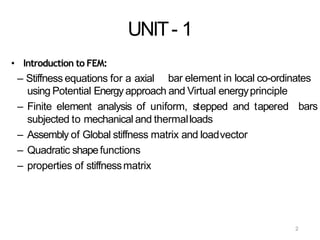
UNIT- 1
• Introduction to FEM:
– Stiffness equations for a axial bar element in local co-ordinates
bars
using Potential Energyapproach and Virtual energyprinciple
– Finite element analysis of uniform, stepped and tapered
subjected to mechanical and thermalloads
– Assembly of Global stiffness matrix and loadvector
– Quadratic shapefunctions
– properties of stiffnessmatrix

2. Axially LoadedBar
Review:
Stress:
Strain:
Deformation:
Stress:
3
Strain:
Deformation:

3. Axially LoadedBar
4
Review:
Stress:
Strain:
Deformation:

4. Axially Loaded Bar – GoverningEquations
and BoundaryConditions
• Differential Equation
• BoundaryCondition Types
• prescribeddisplacement(essential BC)
•prescribedforce/derivative of displacement
(natural BC)
dx  dx
5
d EA(x)
du   f (x) 0 0  x L

5. 6
Axially Loaded Bar –BoundaryConditions
• Examples
• fixed end
• simplesupport
• free end

6. Potential Energy
- Axially loadedbar
- Elasticbody
x
Stretchedbar
• Elastic Potential Energy(PE)
- Spring case
Unstretched spring
PE 0
2
1
2
kx
PE 
undeformed:
deformed:
0
7
PE 0
1 L
PE  Adx
2
2 V
PE 
1
σT
εdv

7. Potential Energy
• Work Potential(WE)
B
L

WP   u  fdx  Pu
0
P
f
f: distributed force over aline
P: point force
u: displacement
A B
• T
otalPotential Energy
L
0 0
1 L
  Adx  u  fdx  PuB
2
• Principle of Minimum PotentialEnergy
Forconservative systems, of all the kinematically admissible displacementfields,
those corresponding to equilibrium extremize the total potential energy. If the
extremum condition is aminimum, the equilibrium state isstable.
8

8. Potential Energy +Rayleigh-RitzApproach
P
f
A B
Example:
Step1: assumeadisplacement field
i
i  1 to n
u  aii x
 is shapefunction / basis function
n is the order ofapproximation
Step2: calculate total potential energy
9

9. Potential Energy +Rayleigh-Ritz
Approach
f
Example:
P
A B
Step3:select ai sothat the total potential energy isminimum
10

10. Galerkin’sMethod
P
f
A
Example:
EA(x)
du
 P
dx xL
d  du
dx 
EA(x)
dx 
 f (x)  0
ux  0 0 dx
w
V
i
 P



 d du
dx 

 

dx xL

du
~
EA(x)
u~x 0 0
f ( x)dV 0

EA(x) 
B
Seekan approximation u
~so
~
In the Galerkin’s method, the weight function is chosen to be the sameasthe shape
function.
11

11. Galerkin’sMethod
P
f
A B
Example:

  f ( x)dV  0
dx 
du
~ 
EA(x)
 dx 
 d 
V
wi 
0 0
 0
L L
dx 0
du~L
du~dw
EA(x) i
dx  wi fdx wi EA(x)
dx dx
1 2 3
1
2
3
12

12. Finite Element Method –Piecewise
Approximation
x
u
x
u
13

13. FEM Formulation of AxiallyLoaded
Bar – Governing Equations
• WeakForm
• Differential Equation
d  du
dx 
EA(x)
dx 
 f (x)  0 0  x L
• Weighted-Integral Formulation
0



 d  du 
w EA(x)   f (x)dx  0
dx  dx 
L
0
L
du 



0  
du  

L
dw 
0   dx
EA(x)
dx
  wf (x)dx  wEA(x)
dx

14

14. Approximation Methods –Finite
Element Method
Example:
Step1: Discretization
Step2: Weakform of oneelement P2
P1
x1 x2
1
1
 0




 x
x 
x
du 
2
du  
 dx
EA(x)
dx
  w(x) f (x)dx  w(x) EA(x)
dx

x2
dw 
   
1 1
2 2






 P w x P  0
dx
EA(x)  w(x) f (x) dx  w x
dx
x2
dw  du  
x1
 15

15. Approximation Methods –Finite
Element Method
Example(cont):
Step3: Choosingshape functions
- linear shapefunctions u  1u12u2
l
x1 x2
x 
 
1
l
2
2
l
1
x  x
x  x
;  
  2
16
2

1
; 2 
1
1 
1
1
2
l
x 
 1l
 x
 
2
x  x  1;

16. Approximation Methods –Finite
Element Method
Example(cont):
Step4: Forming element equation
weak formbecomes
Letw 1
, 1 1 2 1 1
1
1



l
1 u  u 
l
x2
x
x2

x
  EA 2 1
dx   f dx   P   P 0
2
1
l
EA EA
l
x
x
u1  u2  1 f dx  P
1
weak formbecomes
Letw  2
, 2 2 2 2 1
1
1
 

l
u  u 
l
x2
x
x2
1
x
EA 2 1
dx   f dx   P   P  0
1
l
EA
l
EA
x2
x
 u1  u2  2 f dx  P2
1 1 1
2
P f P
x2

     
EA  1 
1u1 
  x1
 
 P   f   P
1  u  x2
l 1
   2   2   2   2 
  fdx

x1 
1 fdx

E,Aare constant
17

17. Approximation Methods –Finite
Element Method
Example(cont):
Step5: Assembling to form systemequation
Approach 1:
Element1: 0 I I I
I I
u f P
E A
lI
 f I
 PI


1
 
1

  
1

1      
   

2
 
2
 
2

0  0
 0
 0 0  0
 0   0 
 0   0 
    
Element2:
1
2 2
f
uII
f II
PII
lII
 0   0 
  
0  0 
E II
AII 0 0 uII
  
II
PII

  
1
    
1

2     


 0 
 

0 

0 

0 

Element3:
1 1
III III III
III
III III III
f P
1 u f P
 0   0 
0   0 
E III
AIII 0 0   0   0   0 
 
      
     1 
0       
 1 1 0 0 uI

1 0
0 0
0 0
0 0 0
1 1
0 1 1 0
0 0 0

0 0 0
 0 0
l 0 0 1 1 u
0 1
   2   2   2 
18

18. Approximation Methods –Finite
Element Method
Example(cont):
Step5: Assembling to form systemequation
Assembled System:
4 4
19
0 0
0
0
I I II II
lI
l
0
l l
l
EII
AII
EII
AII
EIII
AIII
EIII
AIII
lII
0
lIII
EIII
AIII
EIII
AIII
lIII
lIII
 E I
AI
I I
 E A
 lI




 f1 
u1 

EI
AI
E I
AI

E II
AII
II II
 E A
 3  
  
lII
lIII













2 1 2 1
2 1 2 1
I I
II
II III II III
f1 P
1
f III
PIII
   
P1
 f I  PI 
u   f  P  f II 
 P 

 2    2    2     
u   f  P  
f  f P  P
3  3
 
 
 


  

u 
 
 f 
 
P 
 
4  2   2 

19. Approximation Methods –Finite
Element Method
Example(cont):
Step5: Assembling to form systemequation
Approach 2: Element connectivitytable Element 1 Element 2 Element 3
1 1 2 3
2 2 3 4
global node index
(I,J)
local node
(i,j)
ij
20
IJ
k e
 K

20. Approximation Methods –Finite
Element Method
Example(cont):
Step6: Imposing boundary conditions and forming condensesystem
Condensedsystem:
0
lI
lII
lII
lII
0
lIII
lIII
EIII
AIII
lIII
lIII
 E I
AI

E II
AII
II II
 E A 

u2   f2  0
E II
AII

E III
AIII 
E A        
III III
u3   f3  0
 f  P
 u 
 4   


 EII
AII
 

 E III
AIII
  4 
lII

 
  21

21. Approximation Methods –Finite
Element Method
Example(cont):
Step7: solution
Step8: post calculation
2
dx 1
dx
d2
dx
 
du
 u
d1
u
1 1 2 2
u  u   u  2
1
dx
d2
dx
  E  Eu
d1
Eu
22

22. Summary - Major Steps inFEM
• Discretization
• Derivation of element equation
•weak form
•constructform of approximation solution
overone element
•derive finite element model
• Assembling– putting elements together
• Imposingboundary conditions
• Solvingequations
• Postcomputation
23

23. Exercises – LinearElement
Example1:
E=100 GPa,A=1 cm2
24

24. Linear Formulation for BarElement
 
 2   2   12 22 u2 
K
K
K12 u1 
P   f 
P1

 f1 

K11

 1
1
x2

x
i
x2

x
ji i
ij  dx dx 
EA i j
dx  K , f 
where K  f dx
 d d 
x=x1 x=x2
 2
1

x
x=x1 x=x2
u1 u2
P1 P2
f(x)
L= x2-x1
u
x
25

25. Higher Order Formulation for BarElement
u(x) u11(x) u22 (x) u33 (x)
1 3
u1 u3
u
x
u2
2
u1 u4
u
x
u2 u3
1 2 3 4
u(x) u11( x ) u22 ( x ) u33 ( x ) u44 ( x )
u(x) u11( x ) u22 ( x ) u33 ( x ) u44 ( x )  unn ( x )
n
u1 un
u
x
u2 u3 u4
26
…
…
…
…
…
1 2 3 4 …
…
…
…
…

26. Natural Coordinates and InterpolationFunctions
  1
2
, 2 
  1
2
1  
Natural (or Normal)Coordinate:
x=x1 x=x2
=-1 =1
x

x  0 x  l
l /2
x  x  x1
x  x1  x2
  2
1 3
2

1
=-1
2
=1

=-1 =1
1 4
2

=-1 =1
3
2
2
3
2
1
 1
    1  1,  
 1
  ,
2
1

3 

3 16

3

16    
1 ,  
27
 1
1 1

  
9  
1  
1   

27






3

3
16
 
3
16
4
3
  
27
 1
1  1,  
9
 1
1  
1

27. Quadratic Formulation for BarElement
   
i i i
l
2
 f
and f   f dx  
1
1
1
x2
x 1
 d d   d d  2
 dx dx 
1
 d d l
d, i, j  1, 2, 3
where Kij   EA
i
 dx   EA
i
 d  K
j j
ji


 
2 
33  3 
13 23
23 
22
12
3  3 
 2   2 
u 
u 
K
K13 u1 
K11 K12
P   f 
P    f   K K K
K K
P1   f1 
=-1 =0 =1

x2

x1


28

28. Quadratic Formulation for BarElement
u1 u3
u2
f(x)
P3
P1
P2
x1
=-1
x2
=0
x3
=1
2
2
3
2
1
3 3
2 2
1 1
 1
 u  1 1u
 1
)  u  (  ) u
( ) u  (
u( )  u 
2
2
3
2
1
 1
,     1  1,  
  1
 
l l
dx l d dx l d l dx l d
d1

2 d1

2 1
, d2

2 d2
 
4,
d3

2 d3

2 1
l /2
x  x1  x2
  2 l d  dx
2
d 2

dx l
29

29. Exercises – Quadratic Element
30
Example2:
E=100 GPa,A1=1 cm2;A1=2cm2

30. Some Issues
Non-constant crosssection:
Interior loadpoint:
Mixed boundary condition:
k
31