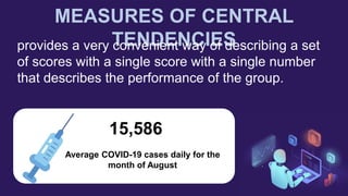
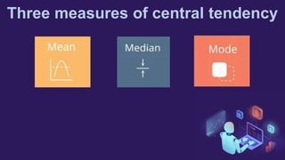
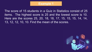
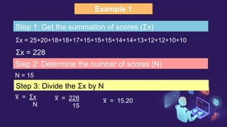
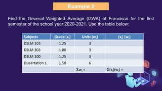
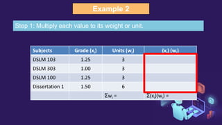
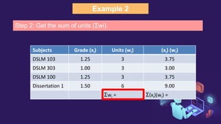
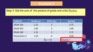
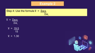
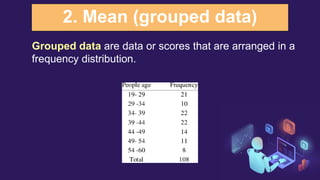
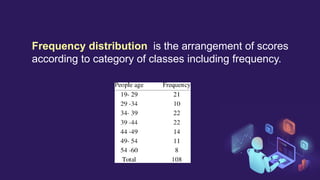
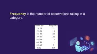
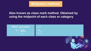
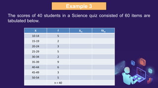
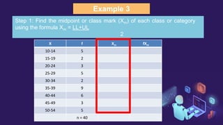
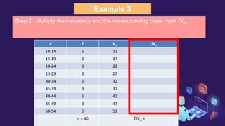
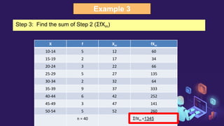
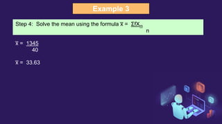
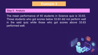
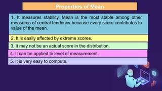
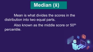
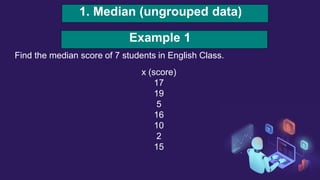
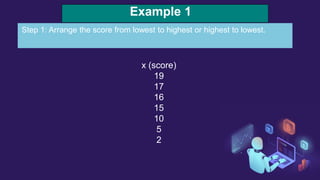
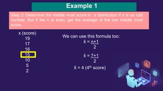
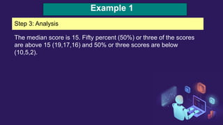
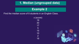
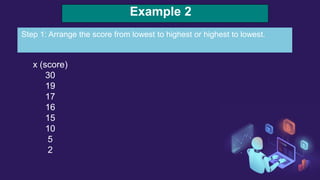
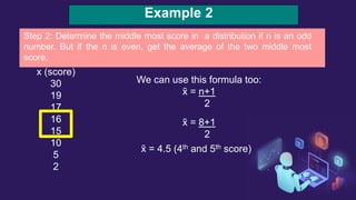
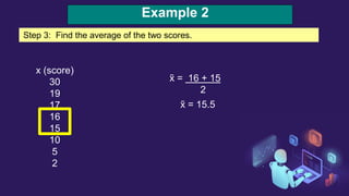
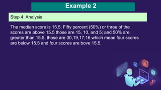
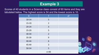
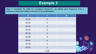
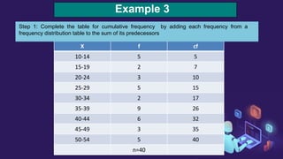
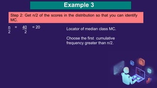
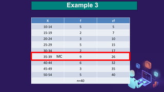
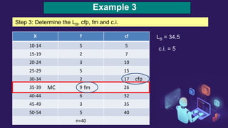
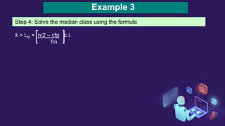
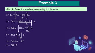
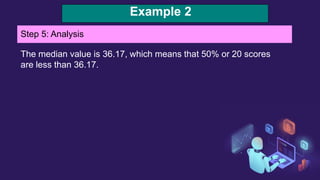
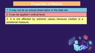
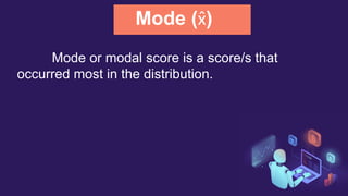
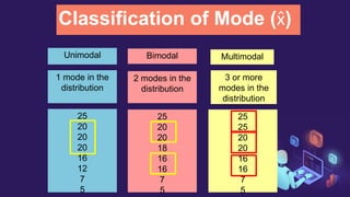
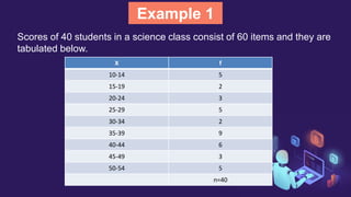
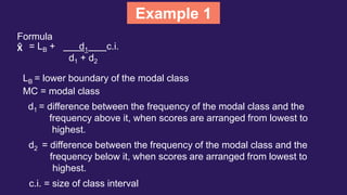
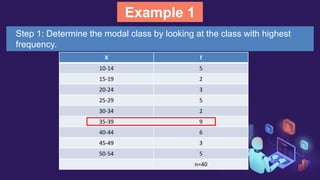
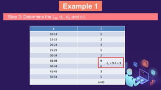
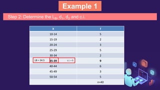
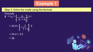
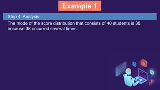
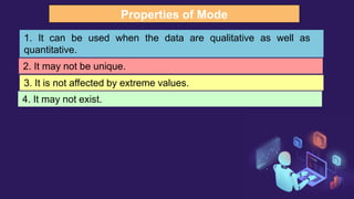
MEASURES OF CENTRAL
TENDENCIE
S
MEASURES OF CENTRAL
TENDENCIES
provides a very convenient way of describing a set
of scores with a single score with a single number
that describes the performance of the group.
15,586
Average COVID-19 cases daily for the
month of August
Three measures of central tendency
Mean (x
̅ )
Mean is the most commonly used measure of
the center data.
Also known as arithmetic average.
1. Mean (ungrouped data)
Population mean
μ = Σx
N
Sample mean
x
̅ = Σx
N
Weighted mean
x
̅ = Σ wi xi
wi
Example 1
The score of 15 students in a Quiz in Statistics consist of 25
items. The highest score is 25 and the lowest score is 10.
Here are the scores 25, 20, 18, 18, 17, 15, 15, 15, 14, 14,
13, 12, 12, 10, 10. Find the mean of the scores.
Example 1
Σx = 25+20+18+18+17+15+15+15+14+14+13+12+12+10+10
Step 1: Get the summation of scores (Σx)
Σx = 228
Step 2: Determine the number of scores (N)
N = 15
Step 3: Divide the Σx by N
x
̅ = Σx
N
x
̅ = 228
15
x
̅ = 15.20
Example 1
Step 4. Analysis
The average performance of 15 students who participated in the quiz
consisting of 25 items is 15.2. The implication of this is that student who
got scores below 15.2 did not perform well in the said examination.
Students who got scores higher than 15.2 performed well in the
examination compared to the performance of the whole class.
Example 2
Find the General Weighted Average (GWA) of Francisco for the first
semester of the school year 2020-2021. Use the table below:
Subjects Grade (xi) Units (wi) (xi) (wi)
DSLM 103 1.25 3
DSLM 303 1.00 3
DSLM 100 1.25 3
Dissertation 1 1.50 6
Σwi = Σ(xi)(wi) =
Example 2
Subjects Grade (xi) Units (wi) (xi) (wi)
DSLM 103 1.25 3
DSLM 303 1.00 3
DSLM 100 1.25 3
Dissertation 1 1.50 6
Σwi = Σ(xi)(wi) =
Step 1: Multiply each value to its weight or unit.
Example 2
Subjects Grade (xi) Units (wi) (xi) (wi)
DSLM 103 1.25 3 3.75
DSLM 303 1.00 3 3.00
DSLM 100 1.25 3 3.75
Dissertation 1 1.50 6 9.00
Σwi = Σ(xi)(wi) =
Step 2: Get the sum of units (Σwi).
Example 2
Subjects Grade (xi) Units (wi) (xi) (wi)
DSLM 103 1.25 3 3.75
DSLM 303 1.00 3 3.00
DSLM 100 1.25 3 3.75
Dissertation 1 1.50 6 9.00
Σwi = 15 Σ(xi)(wi) =
Step 3: Get the sum of the product of grade and units Σ(xi)(wi)
Example 2
Step 4: Use the formula x
̅ = Σwixi
Σwi
x
̅ = Σwixi
Σwi
x
̅ = 19.5
15
x
̅ = 1.30
2. Mean (grouped data)
Grouped data are data or scores that are arranged in a
frequency distribution.
Frequency distribution is the arrangement of scores
according to category of classes including frequency.
Frequency is the number of observations falling in a
category.
Also known as class mark method. Obtained by
using the midpoint of each class or category
Midpoint method
Mean (grouped)
x
̅ = ΣfXm
n
f =
Xm =
n =
Example 3
The scores of 40 students in a Science quiz consisted of 60 items are
tabulated below.
X f Xm fXm
10-14 5
15-19 2
20-24 3
25-29 5
30-34 2
35-39 9
40-44 6
45-49 3
50-54 5
n = 40
Example 3
X f Xm fXm
10-14 5
15-19 2
20-24 3
25-29 5
30-34 2
35-39 9
40-44 6
45-49 3
50-54 5
n = 40
Step 1: Find the midpoint or class mark (Xm) of each class or category
using the formula Xm = LL+UL
2
Example 3
X f Xm fXm
10-14 5 12
15-19 2 17
20-24 3 22
25-29 5 27
30-34 2 32
35-39 9 37
40-44 6 42
45-49 3 47
50-54 5 52
n = 40 ΣfXm =
Step 2: Multiply the frequency and the corresponding class mark fXm
Example 3
X f Xm fXm
10-14 5 12 60
15-19 2 17 34
20-24 3 22 66
25-29 5 27 135
30-34 2 32 64
35-39 9 37 333
40-44 6 42 252
45-49 3 47 141
50-54 5 52 260
n = 40 ΣfXm =1345
Step 3: Find the sum of Step 2 (ΣfXm)
Example 3
Step 4: Solve the mean using the formula x
̅ = ΣfXm
n
x
̅ = 1345
40
x
̅ = 33.63
Example 3
Step 5: Analysis
The mean performance of 40 students in Science quiz is 33.63.
Those students who got scores below 33.63 did not perform well
in the said quiz while those who got scores above 33.63
performed well.
3. Mean using MS Excel
Properties of Mean
1. It measures stability. Mean is the most stable among other
measures of central tendency because every score contributes to
value of the mean.
2. It is easily affected by extreme scores.
3. It may not be an actual score in the distribution.
4. It can be applied to level of measurement.
5. It is very easy to compute.
Median (x̃)
Mean is what divides the scores in the
distribution into two equal parts.
Also known as the middle score or 50th
percentile.
1. Median (ungrouped data)
Find the median score of 7 students in English Class.
Example 1
x (score)
17
19
5
16
10
2
15
Example 1
x (score)
19
17
16
15
10
5
2
Step 1: Arrange the score from lowest to highest or highest to lowest.
Example 1
x (score)
19
17
16
15
10
5
2
Step 2: Determine the middle most score in a distribution if n is an odd
number. But if the n is even, get the average of the two middle most
score,
We can use this formula too:
x̃ = n+1
2
x̃ = 7+1
2
x̃ = 4 (4th score)
Example 1
Step 3: Analysis
The median score is 15. Fifty percent (50%) or three of the scores
are above 15 (19,17,16) and 50% or three scores are below
(10,5,2).
1. Median (ungrouped data)
Find the median score of 8 students in an English Class.
Example 2
x (score)
19
30
17
5
15
10
2
16
Example 2
x (score)
30
19
17
16
15
10
5
2
Step 1: Arrange the score from lowest to highest or highest to lowest.
Example 2
x (score)
30
19
17
16
15
10
5
2
We can use this formula too:
x̃ = n+1
2
x̃ = 8+1
2
x̃ = 4.5 (4th and 5th score)
Step 2: Determine the middle most score in a distribution if n is an odd
number. But if the n is even, get the average of the two middle most
score,
Example 2
x (score)
30
19
17
16
15
10
5
2
x̃ = 16 + 15
2
x̃ = 15.5
Step 3: Find the average of the two scores.
Example 2
Step 4: Analysis
The median score is 15.5. Fifty percent (50%) or three of the
scores are above 15.5 those are 15, 10, and 5; and 50% are
greater than 15.5, those are 30,19,17,16 which mean four scores
are below 15.5 and four scores are bove 15.5.
1. Median (grouped data)
Scores of 40 students in a Science class consist of 60 items and they are
tabulated below. The highest score is 54 and the lowest score is 10.
Example 3
X f cf
10-14 5
15-19 2
20-24 3
25-29 5
30-34 2
35-39 9
40-44 6
45-49 3
50-54 5
n=40
Formula:
Example 3
x̃ = LB + n/2 – cfp c.i.
fm
x̃ = median value
MC = median class is the class with the smallest cumulative frequency greater
than or equal to ½ of the total frequencies.
- a category containing the n/2 (locator)
LB = lower boundary of the median class (MC)
Cfp = cumulative frequency before the median class if the scores are
arranged from lowest to highest value.
fm = Frequency of median class
c.i. size of the class interval
Example 3
X f cf
10-14 5
15-19 2
20-24 3
25-29 5
30-34 2
35-39 9
40-44 6
45-49 3
50-54 5
n=40
Step 1: Complete the table for cumulative frequency by adding each frequency from a
frequency distribution table to the sum of its predecessors
Example 3
X f cf
10-14 5 5
15-19 2 7
20-24 3 10
25-29 5 15
30-34 2 17
35-39 9 26
40-44 6 32
45-49 3 35
50-54 5 40
n=40
Step 1: Complete the table for cumulative frequency by adding each frequency from a
frequency distribution table to the sum of its predecessors
Example 3
Step 2: Get n/2 of the scores in the distribution so that you can identify
MC.
n = 40 = 20
2 2
Locator of median class MC.
Choose the first cumulative
frequency greater than n/2.
Example 3
X f cf
10-14 5 5
15-19 2 7
20-24 3 10
25-29 5 15
30-34 2 17
35-39 9 26
40-44 6 32
45-49 3 35
50-54 5 40
n=40
MC
Example 3
X f cf
10-14 5 5
15-19 2 7
20-24 3 10
25-29 5 15
30-34 2 17
35-39 9 26
40-44 6 32
45-49 3 35
50-54 5 40
n=40
Step 3: Determine the LB, cfp, fm and c.i.
MC fm
cfp
LB = 34.5
c.i. = 5
Example 3
Step 4: Solve the median class using the formula
x̃ = LB + n/2 – cfp c.i.
fm
Example 3
Step 4: Solve the median class using the formula
x̃ = LB + n/2 – cfp c.i.
fm
x̃ = 34.5 + 40/2 – 17 5
9
x̃ = 34.5 + 20 – 17 5
9
x̃ = 34.5 + 3 5
9
x̃ = 34.5 + 1.67
x̃ = 36.17
Example 2
Step 5: Analysis
The median value is 36.17, which means that 50% or 20 scores
are less than 36.17.
Properties of Median
1. It may not be an actual observation in the data set.
2. It can be applied I ordinal level.
3. It is not affected by extreme values because median is a
positional measure.
Mode (x̂)
Mode or modal score is a score/s that
occurred most in the distribution.
Classification of Mode (x̂)
Unimodal Bimodal Multimodal
1 mode in the
distribution
2 modes in the
distribution
3 or more
modes in the
distribution
25
20
20
20
16
12
7
5
25
20
20
18
16
16
7
5
25
25
20
20
16
16
7
5
Mode for grouped data (x̂)
Example 1
Scores of 40 students in a science class consist of 60 items and they are
tabulated below.
X f
10-14 5
15-19 2
20-24 3
25-29 5
30-34 2
35-39 9
40-44 6
45-49 3
50-54 5
n=40
Example 1
Scores of 40 students in a science class consist of 60 items and they are
tabulated below.
X f
10-14 5
15-19 2
20-24 3
25-29 5
30-34 2
35-39 9
40-44 6
45-49 3
50-54 5
n=40
Example 1
Formula
X̂ = LB + d1 c.i.
d1 + d2
LB = lower boundary of the modal class
MC = modal class
d1 = difference between the frequency of the modal class and the
frequency above it, when scores are arranged from lowest to
highest.
d2 = difference between the frequency of the modal class and the
frequency below it, when scores are arranged from lowest to
highest.
c.i. = size of class interval
Example 1
Step 1: Determine the modal class by looking at the class with highest
frequency.
X f
10-14 5
15-19 2
20-24 3
25-29 5
30-34 2
35-39 9
40-44 6
45-49 3
50-54 5
n=40
Example 1
X f
10-14 5
15-19 2
20-24 3
25-29 5
30-34 2
35-39 9
40-44 6
45-49 3
50-54 5
n=40
d1 = 9-2 = 7
Step 2: Determine the LB, d1, d2 and c.i.
Example 1
X f
10-14 5
15-19 2
20-24 3
25-29 5
30-34 2
35-39 9
40-44 6
45-49 3
50-54 5
n=40
d2 = 9-6 = 3
Step 2: Determine the LB, d1, d2 and c.i.
Example 1
Step 2: Determine the LB, d1, d2 and c.i.
X f
10-14 5
15-19 2
20-24 3
25-29 5
30-34 2
35-39 9
40-44 6
45-49 3
50-54 5
n=40
LB = 34.5 c.i. = 5
Example 1
Step 3: Solve the mode using the formula
Formula
X̂ = LB + d1 c.i.
d1 + d2
= 34.4+ 7 5
7 + 3
= 34.4 + 3.5
= 38
Example 1
Step 4: Analysis
The mode of the score distribution that consists of 40 students is 38,
because 38 occurred several times.
Properties of Mode
1. It can be used when the data are qualitative as well as
quantitative.
2. It may not be unique.
3. It is not affected by extreme values.
4. It may not exist.
THANK
YOU
PRESENTERS
MARVIN D. APRITADO
ELLA A. MENDIOLA
MEASURES-OF-CENTRAL-TENDENCIES-1[1] [Autosaved].pptx

MEASURES-OF-CENTRAL-TENDENCIES-1[1] [Autosaved].pptx

  • 1.
  • 2.
    MEASURES OF CENTRAL TENDENCIES providesa very convenient way of describing a set of scores with a single score with a single number that describes the performance of the group. 15,586 Average COVID-19 cases daily for the month of August
  • 3.
    Three measures ofcentral tendency
  • 4.
    Mean (x ̅ ) Meanis the most commonly used measure of the center data. Also known as arithmetic average.
  • 5.
    1. Mean (ungroupeddata) Population mean μ = Σx N Sample mean x ̅ = Σx N Weighted mean x ̅ = Σ wi xi wi
  • 6.
    Example 1 The scoreof 15 students in a Quiz in Statistics consist of 25 items. The highest score is 25 and the lowest score is 10. Here are the scores 25, 20, 18, 18, 17, 15, 15, 15, 14, 14, 13, 12, 12, 10, 10. Find the mean of the scores.
  • 7.
    Example 1 Σx =25+20+18+18+17+15+15+15+14+14+13+12+12+10+10 Step 1: Get the summation of scores (Σx) Σx = 228 Step 2: Determine the number of scores (N) N = 15 Step 3: Divide the Σx by N x ̅ = Σx N x ̅ = 228 15 x ̅ = 15.20
  • 8.
    Example 1 Step 4.Analysis The average performance of 15 students who participated in the quiz consisting of 25 items is 15.2. The implication of this is that student who got scores below 15.2 did not perform well in the said examination. Students who got scores higher than 15.2 performed well in the examination compared to the performance of the whole class.
  • 9.
    Example 2 Find theGeneral Weighted Average (GWA) of Francisco for the first semester of the school year 2020-2021. Use the table below: Subjects Grade (xi) Units (wi) (xi) (wi) DSLM 103 1.25 3 DSLM 303 1.00 3 DSLM 100 1.25 3 Dissertation 1 1.50 6 Σwi = Σ(xi)(wi) =
  • 10.
    Example 2 Subjects Grade(xi) Units (wi) (xi) (wi) DSLM 103 1.25 3 DSLM 303 1.00 3 DSLM 100 1.25 3 Dissertation 1 1.50 6 Σwi = Σ(xi)(wi) = Step 1: Multiply each value to its weight or unit.
  • 11.
    Example 2 Subjects Grade(xi) Units (wi) (xi) (wi) DSLM 103 1.25 3 3.75 DSLM 303 1.00 3 3.00 DSLM 100 1.25 3 3.75 Dissertation 1 1.50 6 9.00 Σwi = Σ(xi)(wi) = Step 2: Get the sum of units (Σwi).
  • 12.
    Example 2 Subjects Grade(xi) Units (wi) (xi) (wi) DSLM 103 1.25 3 3.75 DSLM 303 1.00 3 3.00 DSLM 100 1.25 3 3.75 Dissertation 1 1.50 6 9.00 Σwi = 15 Σ(xi)(wi) = Step 3: Get the sum of the product of grade and units Σ(xi)(wi)
  • 13.
    Example 2 Step 4:Use the formula x ̅ = Σwixi Σwi x ̅ = Σwixi Σwi x ̅ = 19.5 15 x ̅ = 1.30
  • 14.
    2. Mean (groupeddata) Grouped data are data or scores that are arranged in a frequency distribution.
  • 15.
    Frequency distribution isthe arrangement of scores according to category of classes including frequency.
  • 16.
    Frequency is thenumber of observations falling in a category.
  • 17.
    Also known asclass mark method. Obtained by using the midpoint of each class or category Midpoint method Mean (grouped) x ̅ = ΣfXm n f = Xm = n =
  • 18.
    Example 3 The scoresof 40 students in a Science quiz consisted of 60 items are tabulated below. X f Xm fXm 10-14 5 15-19 2 20-24 3 25-29 5 30-34 2 35-39 9 40-44 6 45-49 3 50-54 5 n = 40
  • 19.
    Example 3 X fXm fXm 10-14 5 15-19 2 20-24 3 25-29 5 30-34 2 35-39 9 40-44 6 45-49 3 50-54 5 n = 40 Step 1: Find the midpoint or class mark (Xm) of each class or category using the formula Xm = LL+UL 2
  • 20.
    Example 3 X fXm fXm 10-14 5 12 15-19 2 17 20-24 3 22 25-29 5 27 30-34 2 32 35-39 9 37 40-44 6 42 45-49 3 47 50-54 5 52 n = 40 ΣfXm = Step 2: Multiply the frequency and the corresponding class mark fXm
  • 21.
    Example 3 X fXm fXm 10-14 5 12 60 15-19 2 17 34 20-24 3 22 66 25-29 5 27 135 30-34 2 32 64 35-39 9 37 333 40-44 6 42 252 45-49 3 47 141 50-54 5 52 260 n = 40 ΣfXm =1345 Step 3: Find the sum of Step 2 (ΣfXm)
  • 22.
    Example 3 Step 4:Solve the mean using the formula x ̅ = ΣfXm n x ̅ = 1345 40 x ̅ = 33.63
  • 23.
    Example 3 Step 5:Analysis The mean performance of 40 students in Science quiz is 33.63. Those students who got scores below 33.63 did not perform well in the said quiz while those who got scores above 33.63 performed well.
  • 24.
    3. Mean usingMS Excel
  • 25.
    Properties of Mean 1.It measures stability. Mean is the most stable among other measures of central tendency because every score contributes to value of the mean. 2. It is easily affected by extreme scores. 3. It may not be an actual score in the distribution. 4. It can be applied to level of measurement. 5. It is very easy to compute.
  • 26.
    Median (x̃) Mean iswhat divides the scores in the distribution into two equal parts. Also known as the middle score or 50th percentile.
  • 27.
    1. Median (ungroupeddata) Find the median score of 7 students in English Class. Example 1 x (score) 17 19 5 16 10 2 15
  • 28.
    Example 1 x (score) 19 17 16 15 10 5 2 Step1: Arrange the score from lowest to highest or highest to lowest.
  • 29.
    Example 1 x (score) 19 17 16 15 10 5 2 Step2: Determine the middle most score in a distribution if n is an odd number. But if the n is even, get the average of the two middle most score, We can use this formula too: x̃ = n+1 2 x̃ = 7+1 2 x̃ = 4 (4th score)
  • 30.
    Example 1 Step 3:Analysis The median score is 15. Fifty percent (50%) or three of the scores are above 15 (19,17,16) and 50% or three scores are below (10,5,2).
  • 31.
    1. Median (ungroupeddata) Find the median score of 8 students in an English Class. Example 2 x (score) 19 30 17 5 15 10 2 16
  • 32.
    Example 2 x (score) 30 19 17 16 15 10 5 2 Step1: Arrange the score from lowest to highest or highest to lowest.
  • 33.
    Example 2 x (score) 30 19 17 16 15 10 5 2 Wecan use this formula too: x̃ = n+1 2 x̃ = 8+1 2 x̃ = 4.5 (4th and 5th score) Step 2: Determine the middle most score in a distribution if n is an odd number. But if the n is even, get the average of the two middle most score,
  • 34.
    Example 2 x (score) 30 19 17 16 15 10 5 2 x̃= 16 + 15 2 x̃ = 15.5 Step 3: Find the average of the two scores.
  • 35.
    Example 2 Step 4:Analysis The median score is 15.5. Fifty percent (50%) or three of the scores are above 15.5 those are 15, 10, and 5; and 50% are greater than 15.5, those are 30,19,17,16 which mean four scores are below 15.5 and four scores are bove 15.5.
  • 36.
  • 37.
    Scores of 40students in a Science class consist of 60 items and they are tabulated below. The highest score is 54 and the lowest score is 10. Example 3 X f cf 10-14 5 15-19 2 20-24 3 25-29 5 30-34 2 35-39 9 40-44 6 45-49 3 50-54 5 n=40
  • 38.
    Formula: Example 3 x̃ =LB + n/2 – cfp c.i. fm x̃ = median value MC = median class is the class with the smallest cumulative frequency greater than or equal to ½ of the total frequencies. - a category containing the n/2 (locator) LB = lower boundary of the median class (MC) Cfp = cumulative frequency before the median class if the scores are arranged from lowest to highest value. fm = Frequency of median class c.i. size of the class interval
  • 39.
    Example 3 X fcf 10-14 5 15-19 2 20-24 3 25-29 5 30-34 2 35-39 9 40-44 6 45-49 3 50-54 5 n=40 Step 1: Complete the table for cumulative frequency by adding each frequency from a frequency distribution table to the sum of its predecessors
  • 40.
    Example 3 X fcf 10-14 5 5 15-19 2 7 20-24 3 10 25-29 5 15 30-34 2 17 35-39 9 26 40-44 6 32 45-49 3 35 50-54 5 40 n=40 Step 1: Complete the table for cumulative frequency by adding each frequency from a frequency distribution table to the sum of its predecessors
  • 41.
    Example 3 Step 2:Get n/2 of the scores in the distribution so that you can identify MC. n = 40 = 20 2 2 Locator of median class MC. Choose the first cumulative frequency greater than n/2.
  • 42.
    Example 3 X fcf 10-14 5 5 15-19 2 7 20-24 3 10 25-29 5 15 30-34 2 17 35-39 9 26 40-44 6 32 45-49 3 35 50-54 5 40 n=40 MC
  • 43.
    Example 3 X fcf 10-14 5 5 15-19 2 7 20-24 3 10 25-29 5 15 30-34 2 17 35-39 9 26 40-44 6 32 45-49 3 35 50-54 5 40 n=40 Step 3: Determine the LB, cfp, fm and c.i. MC fm cfp LB = 34.5 c.i. = 5
  • 44.
    Example 3 Step 4:Solve the median class using the formula x̃ = LB + n/2 – cfp c.i. fm
  • 45.
    Example 3 Step 4:Solve the median class using the formula x̃ = LB + n/2 – cfp c.i. fm x̃ = 34.5 + 40/2 – 17 5 9 x̃ = 34.5 + 20 – 17 5 9 x̃ = 34.5 + 3 5 9 x̃ = 34.5 + 1.67 x̃ = 36.17
  • 46.
    Example 2 Step 5:Analysis The median value is 36.17, which means that 50% or 20 scores are less than 36.17.
  • 47.
    Properties of Median 1.It may not be an actual observation in the data set. 2. It can be applied I ordinal level. 3. It is not affected by extreme values because median is a positional measure.
  • 48.
    Mode (x̂) Mode ormodal score is a score/s that occurred most in the distribution.
  • 49.
    Classification of Mode(x̂) Unimodal Bimodal Multimodal 1 mode in the distribution 2 modes in the distribution 3 or more modes in the distribution 25 20 20 20 16 12 7 5 25 20 20 18 16 16 7 5 25 25 20 20 16 16 7 5
  • 50.
    Mode for groupeddata (x̂)
  • 51.
    Example 1 Scores of40 students in a science class consist of 60 items and they are tabulated below. X f 10-14 5 15-19 2 20-24 3 25-29 5 30-34 2 35-39 9 40-44 6 45-49 3 50-54 5 n=40
  • 52.
    Example 1 Scores of40 students in a science class consist of 60 items and they are tabulated below. X f 10-14 5 15-19 2 20-24 3 25-29 5 30-34 2 35-39 9 40-44 6 45-49 3 50-54 5 n=40
  • 53.
    Example 1 Formula X̂ =LB + d1 c.i. d1 + d2 LB = lower boundary of the modal class MC = modal class d1 = difference between the frequency of the modal class and the frequency above it, when scores are arranged from lowest to highest. d2 = difference between the frequency of the modal class and the frequency below it, when scores are arranged from lowest to highest. c.i. = size of class interval
  • 54.
    Example 1 Step 1:Determine the modal class by looking at the class with highest frequency. X f 10-14 5 15-19 2 20-24 3 25-29 5 30-34 2 35-39 9 40-44 6 45-49 3 50-54 5 n=40
  • 55.
    Example 1 X f 10-145 15-19 2 20-24 3 25-29 5 30-34 2 35-39 9 40-44 6 45-49 3 50-54 5 n=40 d1 = 9-2 = 7 Step 2: Determine the LB, d1, d2 and c.i.
  • 56.
    Example 1 X f 10-145 15-19 2 20-24 3 25-29 5 30-34 2 35-39 9 40-44 6 45-49 3 50-54 5 n=40 d2 = 9-6 = 3 Step 2: Determine the LB, d1, d2 and c.i.
  • 57.
    Example 1 Step 2:Determine the LB, d1, d2 and c.i. X f 10-14 5 15-19 2 20-24 3 25-29 5 30-34 2 35-39 9 40-44 6 45-49 3 50-54 5 n=40 LB = 34.5 c.i. = 5
  • 58.
    Example 1 Step 3:Solve the mode using the formula Formula X̂ = LB + d1 c.i. d1 + d2 = 34.4+ 7 5 7 + 3 = 34.4 + 3.5 = 38
  • 59.
    Example 1 Step 4:Analysis The mode of the score distribution that consists of 40 students is 38, because 38 occurred several times.
  • 60.
    Properties of Mode 1.It can be used when the data are qualitative as well as quantitative. 2. It may not be unique. 3. It is not affected by extreme values. 4. It may not exist.
  • 61.