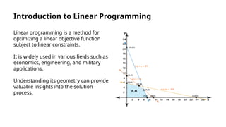
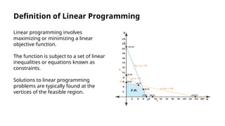
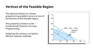
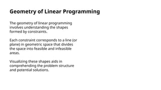
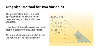
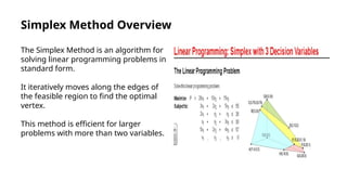
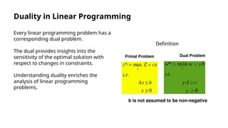
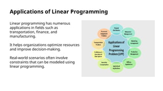
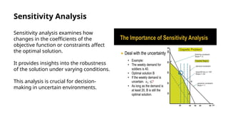
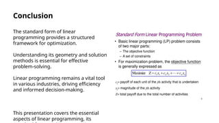
Linear programming is a method for optimizing a linear objective function subject to linear constraints, and is applicable in fields such as economics, engineering, and military. The standard form of a problem maximizes an objective function with constraints expressed as equalities and includes non-negativity conditions. Understanding the geometry of linear programming, as well as solution methods like the simplex method and sensitivity analysis, is crucial for effective application and analysis.