Download free for 30 days
Sign in
Upload
Language (EN)
Support
Business
Mobile
Social Media
Marketing
Technology
Art & Photos
Career
Design
Education
Presentations & Public Speaking
Government & Nonprofit
Healthcare
Internet
Law
Leadership & Management
Automotive
Engineering
Software
Recruiting & HR
Retail
Sales
Services
Science
Small Business & Entrepreneurship
Food
Environment
Economy & Finance
Data & Analytics
Investor Relations
Sports
Spiritual
News & Politics
Travel
Self Improvement
Real Estate
Entertainment & Humor
Health & Medicine
Devices & Hardware
Lifestyle
Change Language
Language
English
Español
Português
Français
Deutsche
Cancel
Save
Submit search
EN
Uploaded by
AchrafBoura
32 views
SPC QUALITY MANUFACTURING PROCESS PRODUCTION
Quality
Science
◦
Read more
0
Save
Share
Embed
Embed presentation
Download
Download to read offline
1
/ 23
2
/ 23
Most read
3
/ 23
4
/ 23
5
/ 23
6
/ 23
7
/ 23
8
/ 23
9
/ 23
10
/ 23
11
/ 23
12
/ 23
13
/ 23
14
/ 23
15
/ 23
16
/ 23
17
/ 23
18
/ 23
19
/ 23
20
/ 23
21
/ 23
22
/ 23
23
/ 23
More Related Content
PDF
Hızlı Ozet - Istatistiksel Proses Kontrol
by
metallicaslayer
PDF
Statistical Process Control Presentation.pdf
by
newaybeyene5
PPT
Spc
by
Jitesh Gaurav
PDF
5. spc control charts
by
Hakeem-Ur- Rehman
PPTX
Statistical Process Control,Control Chart and Process Capability
by
vaidehishah25
PPTX
STATISTICAL PROCESS CONTROL(PPT).pptx
by
mayankdubey99
PDF
Six sigma
by
Alaleh Irooni
DOCX
Lecture 3 Statistical ProcessControl (SPC).docx
by
smile790243
Hızlı Ozet - Istatistiksel Proses Kontrol
by
metallicaslayer
Statistical Process Control Presentation.pdf
by
newaybeyene5
Spc
by
Jitesh Gaurav
5. spc control charts
by
Hakeem-Ur- Rehman
Statistical Process Control,Control Chart and Process Capability
by
vaidehishah25
STATISTICAL PROCESS CONTROL(PPT).pptx
by
mayankdubey99
Six sigma
by
Alaleh Irooni
Lecture 3 Statistical ProcessControl (SPC).docx
by
smile790243
Similar to SPC QUALITY MANUFACTURING PROCESS PRODUCTION
PPT
Chapter 1 spc
by
Jitesh Gaurav
PPT
Introduction to SPC
by
Lorraine Fraser, MBA, M.Eng., P.Eng.
PPT
Introduction To SPC
by
LN Mishra CBAP
PPTX
statistical process control
by
AnkitaGorhe
PPT
08 NEM (SPC).ppt
by
SanjeevPawar15
PPTX
SPC Basics Training V1 By Carlos Sanchez
by
Carlos Sanchez
PPT
Statistical Process Control & Control Chart
by
Shekhar Verma
PPTX
Statistical process control (spc)
by
Ashish Chaudhari
PPTX
Control estadistico de calidad
by
ericktc
PPT
QMC chapter four 1.ppt statical quality control
by
dejene1234567
PPT
405chapter5.ppt
by
princeroy73
PPTX
4. CONTROL PHASE.pptx
by
nirajchaudhari27
PPTX
SPC and Control Charts
by
Miguel Montenegro Araujo
PDF
Spc overview mfg
by
innobun
PPTX
Statistical process control (spc)
by
Ashish Chaudhari
PPTX
Statistical Process Control in Operation Mnagement
by
TARUNKUMAR554626
PDF
statisticalprocesscontrol-130116034459-phpapp02.pdf
by
BanshiMedicareExport
PPTX
SATISTICAL PROCESS CONTROL(SPC)
by
VALARMADHIA
PPTX
Mark Harrison SPC Implementation
by
Mark Harrison
PDF
Spc overview mfg
by
James Yencho
Chapter 1 spc
by
Jitesh Gaurav
Introduction to SPC
by
Lorraine Fraser, MBA, M.Eng., P.Eng.
Introduction To SPC
by
LN Mishra CBAP
statistical process control
by
AnkitaGorhe
08 NEM (SPC).ppt
by
SanjeevPawar15
SPC Basics Training V1 By Carlos Sanchez
by
Carlos Sanchez
Statistical Process Control & Control Chart
by
Shekhar Verma
Statistical process control (spc)
by
Ashish Chaudhari
Control estadistico de calidad
by
ericktc
QMC chapter four 1.ppt statical quality control
by
dejene1234567
405chapter5.ppt
by
princeroy73
4. CONTROL PHASE.pptx
by
nirajchaudhari27
SPC and Control Charts
by
Miguel Montenegro Araujo
Spc overview mfg
by
innobun
Statistical process control (spc)
by
Ashish Chaudhari
Statistical Process Control in Operation Mnagement
by
TARUNKUMAR554626
statisticalprocesscontrol-130116034459-phpapp02.pdf
by
BanshiMedicareExport
SATISTICAL PROCESS CONTROL(SPC)
by
VALARMADHIA
Mark Harrison SPC Implementation
by
Mark Harrison
Spc overview mfg
by
James Yencho
Recently uploaded
PDF
Markups, Labor Market Inequality and the Nature of Work
by
GRAPE
PDF
HND Networking and Cloud Computing (NCC).pdf
by
ssuser8dcccc
PPSX
Hot Stage Microscopy Application for Research .ppsx
by
gyaneshsingh86
PPTX
Psychopathology and mental Disorders.pptx
by
Max Annani-Akollor
PDF
Mechanical Properties of Fluids (Prashant Kirad).pdf
by
arleenaulakh97
PDF
12th Bio NCERT Important Questions @irfanullah_ mehar.pdf
by
World of Wisdom
PPTX
Travis Hills of Minnesota Championing a Greener Future Through AI-Driven Pyro...
by
Travis Hills MN
PDF
GENE THERAPY ENHANCING NEUROPLASTICITY FOR BIPOLAR DISORDER
by
PrajaktaPanda
PPTX
genesilencing and gene engineering of technilogy
by
mhossainkhan2022
PDF
Periodic Table Jwala Notes.pdf................
by
akshaybansal243
PPT
Lesson_Presentation_Adding_and_Subtracting_Polynomials (1).ppt
by
engabdelaziz1993
PPTX
ALLOSTERIC INHIBITION : ITS CHARACTERISTICS, STRUCTURE AND MECHANISMS
by
aubrey02judd
PPTX
Lecture 3_CellStructureFunction_2025.pptx
by
AngelMaria66
PPTX
PRE NATAL GROWTH OF MAXILLA in orthodontics.pptx
by
haranip03
PPTX
Trusted Industrial Ammonia Supply – Contact Us
by
mysoreammoniaseo
PPTX
PPt Fisheries and Aquaculture.pptx course
by
tigistafework
PPTX
cellstructurefunction-190628175900..PPTX
by
AubreyDilla
PPTX
All-About-Missiles-----------------.pptx
by
OmkarWandhekar
PPTX
HEPATITIS C: STRUCTURE, GENOME, PATHOGENESIS, DIAGNOSIS, PREVENTION AND TREAT...
by
BIOSPHERE OF KNOWLEDGE
PPTX
Neuropsychology Brain basics history of neuro
by
manju108aug
Markups, Labor Market Inequality and the Nature of Work
by
GRAPE
HND Networking and Cloud Computing (NCC).pdf
by
ssuser8dcccc
Hot Stage Microscopy Application for Research .ppsx
by
gyaneshsingh86
Psychopathology and mental Disorders.pptx
by
Max Annani-Akollor
Mechanical Properties of Fluids (Prashant Kirad).pdf
by
arleenaulakh97
12th Bio NCERT Important Questions @irfanullah_ mehar.pdf
by
World of Wisdom
Travis Hills of Minnesota Championing a Greener Future Through AI-Driven Pyro...
by
Travis Hills MN
GENE THERAPY ENHANCING NEUROPLASTICITY FOR BIPOLAR DISORDER
by
PrajaktaPanda
genesilencing and gene engineering of technilogy
by
mhossainkhan2022
Periodic Table Jwala Notes.pdf................
by
akshaybansal243
Lesson_Presentation_Adding_and_Subtracting_Polynomials (1).ppt
by
engabdelaziz1993
ALLOSTERIC INHIBITION : ITS CHARACTERISTICS, STRUCTURE AND MECHANISMS
by
aubrey02judd
Lecture 3_CellStructureFunction_2025.pptx
by
AngelMaria66
PRE NATAL GROWTH OF MAXILLA in orthodontics.pptx
by
haranip03
Trusted Industrial Ammonia Supply – Contact Us
by
mysoreammoniaseo
PPt Fisheries and Aquaculture.pptx course
by
tigistafework
cellstructurefunction-190628175900..PPTX
by
AubreyDilla
All-About-Missiles-----------------.pptx
by
OmkarWandhekar
HEPATITIS C: STRUCTURE, GENOME, PATHOGENESIS, DIAGNOSIS, PREVENTION AND TREAT...
by
BIOSPHERE OF KNOWLEDGE
Neuropsychology Brain basics history of neuro
by
manju108aug
SPC QUALITY MANUFACTURING PROCESS PRODUCTION
1.
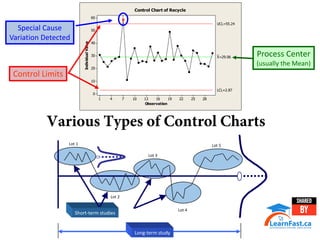
Observation Individual Value 28 25 22 19 16 13 10 7 4 1 60 50 40 30 20 10 0 _ X=29.06 UCL=55.24 LCL=2.87 1 Control Chart of
Recycle Process Center (usually the Mean) Special Cause Variation Detected Control Limits Various Types of Control Charts Lot 1 Lot 2 Lot 3 Lot 4 Lot 5 Short-term studies Long-term study
2.
© Open Source
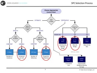
Six Sigma, LLC 3 SPC Selection Process Choose Appropriate Control Chart type of data type of attribute data subgroup size I – MR Chart X – R Chart X – S Chart CumSum Chart EWMA Chart C Chart U Chart NP Chart P Chart type of defect type of subgroups ATTRIBUTE CONTINUOUS DEFECTS DEFECTIVES VARIABLE CONSTANT CONSTANT VARIABLE 1 2-5 10+ Number of Incidences Incidences per Unit Number of Defectives Proportion Defectives Individuals & Moving Range Mean & Range Mean & Std. Dev. Cumulative Sum Exponentially Weighted Moving Average SPECIAL CASES Sample size
3.
© Open Source
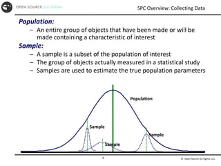
Six Sigma, LLC 4 SPC Overview: Collecting Data Population: – An entire group of objects that have been made or will be made containing a characteristic of interest Sample: – A sample is a subset of the population of interest – The group of objects actually measured in a statistical study – Samples are used to estimate the true population parameters Population Sample Sample Sample
4.
© Open Source
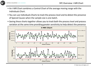
Six Sigma, LLC 5 SPC Overview: I-MR Chart • An I-MR Chart combines a Control Chart of the average moving range with the Individuals Chart. • You can use Individuals Charts to track the process level and to detect the presence of Special Causes when the sample size is one batch. • Seeing these charts together allows you to track both the process level and process variation at the same time providing greater sensitivity to help detect the presence of Special Causes. 109 97 85 73 61 49 37 25 13 1 225.0 222.5 220.0 217.5 215.0 O bser vation Individual Value _ X=219.89 U C L=226.12 LC L=213.67 109 97 85 73 61 49 37 25 13 1 8 6 4 2 0 O bser vation Moving Range __ M R=2.341 U C L=7.649 LC L=0 I-MR Chart
5.
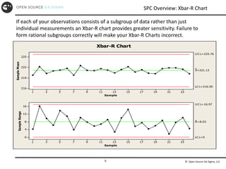
© Open Source
Six Sigma, LLC 6 SPC Overview: Xbar-R Chart If each of your observations consists of a subgroup of data rather than just individual measurements an Xbar-R chart provides greater sensitivity. Failure to form rational subgroups correctly will make your Xbar-R Charts incorrect. 23 21 19 17 15 13 11 9 7 5 3 1 225 222 219 216 Sample Sample Mean _ _ X=221.13 UC L=225.76 LC L=216.50 23 21 19 17 15 13 11 9 7 5 3 1 16 12 8 4 0 Sample Sample Range UC L=16.97 LC L=0 _ R=8.03 Xbar-R Chart
6.
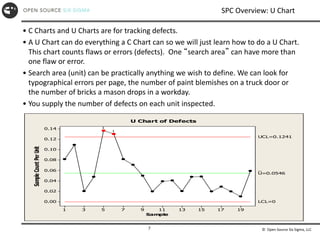
© Open Source
Six Sigma, LLC 7 SPC Overview: U Chart • C Charts and U Charts are for tracking defects. • A U Chart can do everything a C Chart can so we will just learn how to do a U Chart. This chart counts flaws or errors (defects). One “search area” can have more than one flaw or error. • Search area (unit) can be practically anything we wish to define. We can look for typographical errors per page, the number of paint blemishes on a truck door or the number of bricks a mason drops in a workday. • You supply the number of defects on each unit inspected. 19 17 15 13 11 9 7 5 3 1 0.14 0.12 0.10 0.08 0.06 0.04 0.02 0.00 Sample Sample Count Per Unit _ U=0.0546 UCL=0.1241 LCL=0 1 1 U Chart of Defects
7.
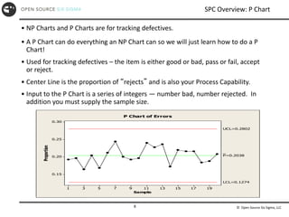
© Open Source
Six Sigma, LLC 8 SPC Overview: P Chart • NP Charts and P Charts are for tracking defectives. • A P Chart can do everything an NP Chart can so we will just learn how to do a P Chart! • Used for tracking defectives – the item is either good or bad, pass or fail, accept or reject. • Center Line is the proportion of “rejects” and is also your Process Capability. • Input to the P Chart is a series of integers — number bad, number rejected. In addition you must supply the sample size. 19 17 15 13 11 9 7 5 3 1 0.30 0.25 0.20 0.15 Sample Proportion _ P=0.2038 UCL=0.2802 LCL=0.1274 P Chart of Errors
8.
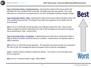
© Open Source
Six Sigma, LLC 9 Type 1 Corrective Action = Countermeasure: improvement made to the process which will eliminate the error condition from occurring. The defect will never be created. This is also referred to as a long-term corrective action in the form of Mistake Proofing or design changes. Type 2 Corrective Action = Flag: improvement made to the process which will detect when the error condition has occurred. This flag will shut down the equipment so the defect will not move forward. SPC on X’s or Y’s with fully trained operators and staff who respect the rules. Once a chart signals a problem everyone understands the rules of SPC and agrees to shut down for Special Cause identification. (Cpk > certain level). Type 3 Corrective Action = Inspection: implementation of a short-term containment which is likely to detect the defect caused by the error condition. Containments are typically audits or 100% inspection. SPC on X’s or Y’s with fully trained operators. The operators have been trained and understand the rules of SPC, but management will not empower them to stop for investigation. S.O.P. is implemented to attempt to detect the defects. This action is not sustainable short- term or long-term. SPC on X’s or Y’s without proper usage = WALL PAPER. SPC Overview: Control Methods/Effectiveness
9.
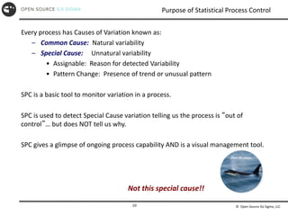
© Open Source
Six Sigma, LLC 10 Purpose of Statistical Process Control Not this special cause!! Every process has Causes of Variation known as: – Common Cause: Natural variability – Special Cause: Unnatural variability • Assignable: Reason for detected Variability • Pattern Change: Presence of trend or unusual pattern SPC is a basic tool to monitor variation in a process. SPC is used to detect Special Cause variation telling us the process is “out of control”… but does NOT tell us why. SPC gives a glimpse of ongoing process capability AND is a visual management tool.
10.
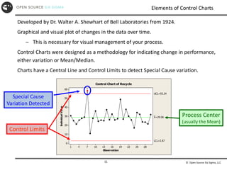
© Open Source
Six Sigma, LLC 11 Elements of Control Charts Observation Individual Value 28 25 22 19 16 13 10 7 4 1 60 50 40 30 20 10 0 _ X=29.06 UCL=55.24 LCL=2.87 1 Control Chart of Recycle Developed by Dr. Walter A. Shewhart of Bell Laboratories from 1924. Graphical and visual plot of changes in the data over time. – This is necessary for visual management of your process. Control Charts were designed as a methodology for indicating change in performance, either variation or Mean/Median. Charts have a Central Line and Control Limits to detect Special Cause variation. Process Center (usually the Mean) Special Cause Variation Detected Control Limits
11.
© Open Source
Six Sigma, LLC 12 Understanding the Power of SPC Control Charts indicate when a process is “out of control” or exhibiting Special Cause variation but NOT why! SPC Charts incorporate upper and lower Control Limits. – The limits are typically +/- 3 from the Center Line. – These limits represent 99.73% of natural variability for Normal Distributions. SPC Charts allow workers and supervision to maintain improved process performance from Lean Six Sigma projects. Use of SPC Charts can be applied to all processes. – Services, manufacturing and retail are just a few industries with SPC applications. – Caution must be taken with use of SPC for Non-normal processes. Control Limits describe the process variability and are unrelated to customer specifications. (Voice of the Process instead of Voice of the Customer) – An undesirable situation is having Control Limits wider than customer specification limits. This will exist for poorly performing processes with a Cp less than 1.0 Many SPC Charts exist and selection must be appropriate for effectiveness.
12.
© Open Source
Six Sigma, LLC 13 The Control Chart Cookbook General Steps for Constructing Control Charts 1. Select characteristic (Critical “X” or CTQ) to be charted. 2. Determine the purpose of the chart. 3. Select data-collection points. 4. Establish the basis for sub-grouping (only for Y’s). 5. Select the type of Control Chart. 6. Determine the measurement method/criteria. 7. Establish the sampling interval/frequency. 8. Determine the sample size. 9. Establish the basis of calculating the Control Limits. 10. Set up the forms or software for charting data. 11. Set up the forms or software for collecting data. 12. Prepare written instructions for all phases. 13. Conduct the necessary training. Stirred or Shaken?
13.
© Open Source
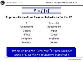
Six Sigma, LLC 14 Focus of Six Sigma and the Use of SPC To get results should we focus our behavior on the Y or X? Y Dependent Output Effect Symptom Monitor X1 . . . XN Independent Input Cause Problem Control When we find the “vital few” X’s first consider using SPC on the X’s to achieve a desired Y. Y = f (x)
14.
© Open Source
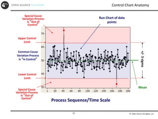
Six Sigma, LLC 15 Control Chart Anatomy Common Cause Variation Process is “In Control” Special Cause Variation Process is “Out of Control” Special Cause Variation Process is “Out of Control” Run Chart of data points Process Sequence/Time Scale Lower Control Limit Mean +/- 3 sigma Upper Control Limit
15.
© Open Source
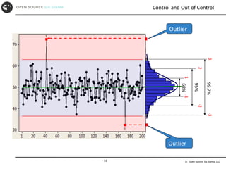
Six Sigma, LLC 16 Control and Out of Control Outlier Outlier 68% 95% 99.7% 3 2 1 -1 -2 -3
16.
© Open Source
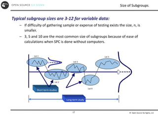
Six Sigma, LLC 17 Size of Subgroups Typical subgroup sizes are 3-12 for variable data: – If difficulty of gathering sample or expense of testing exists the size, n, is smaller. – 3, 5 and 10 are the most common size of subgroups because of ease of calculations when SPC is done without computers. Lot 1 Lot 2 Lot 3 Lot 4 Lot 5 Short-term studies Long-term study
17.
© Open Source
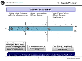
Six Sigma, LLC 18 The Impact of Variation - Natural Process Variation as defined by subgroup selection - Natural Process Variation - Different Operators - Natural Process Variation - Different Operators - Supplier Source And, of course, if two additional sources of variation arrive we will detect that too! First select the spread we will declare as the “Natural Process Variation” so whenever any point lands outside these “Control Limits” an alarm will sound So when a second source of variation appears we will know! If you base your limits on all three sources of variation, what will sound the alarm? -UCL -LCL Sources of Variation
18.
© Open Source
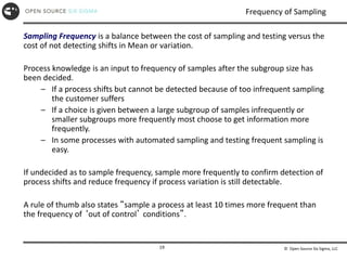
Six Sigma, LLC 19 Frequency of Sampling Sampling Frequency is a balance between the cost of sampling and testing versus the cost of not detecting shifts in Mean or variation. Process knowledge is an input to frequency of samples after the subgroup size has been decided. – If a process shifts but cannot be detected because of too infrequent sampling the customer suffers – If a choice is given between a large subgroup of samples infrequently or smaller subgroups more frequently most choose to get information more frequently. – In some processes with automated sampling and testing frequent sampling is easy. If undecided as to sample frequency, sample more frequently to confirm detection of process shifts and reduce frequency if process variation is still detectable. A rule of thumb also states “sample a process at least 10 times more frequent than the frequency of ‘out of control’ conditions”.
19.
© Open Source
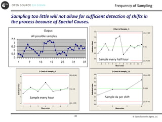
Six Sigma, LLC 20 Frequency of Sampling Output 5 5.5 6 6.5 7 7.5 1 7 13 19 25 31 37 Sampling too little will not allow for sufficient detection of shifts in the process because of Special Causes. Observation Individual Value 13 12 11 10 9 8 7 6 5 4 3 2 1 7.5 7.0 6.5 6.0 5.5 5.0 _ X=6.1 UCL=7.385 LCL=4.815 I Chart of Sample_3 Observation Individual Value 7 6 5 4 3 2 1 8 7 6 5 4 _ X=6.129 UCL=8.168 LCL=4.090 I Chart of Sample_6 Observation Individual Value 4 3 2 1 6.6 6.4 6.2 6.0 5.8 5.6 5.4 5.2 5.0 _ X=5.85 UCL=6.559 LCL=5.141 I Chart of Sample_12 All possible samples Sample every hour Sample 4x per shift Sample every half hour
20.
© Open Source
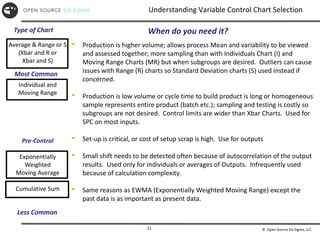
Six Sigma, LLC 21 Understanding Variable Control Chart Selection Type of Chart When do you need it? Production is higher volume; allows process Mean and variability to be viewed and assessed together; more sampling than with Individuals Chart (I) and Moving Range Charts (MR) but when subgroups are desired. Outliers can cause issues with Range (R) charts so Standard Deviation charts (S) used instead if concerned. Production is low volume or cycle time to build product is long or homogeneous sample represents entire product (batch etc.); sampling and testing is costly so subgroups are not desired. Control limits are wider than Xbar Charts. Used for SPC on most inputs. Set-up is critical, or cost of setup scrap is high. Use for outputs Small shift needs to be detected often because of autocorrelation of the output results. Used only for individuals or averages of Outputs. Infrequently used because of calculation complexity. Same reasons as EWMA (Exponentially Weighted Moving Range) except the past data is as important as present data. Average & Range or S (Xbar and R or Xbar and S) Individual and Moving Range Pre-Control Exponentially Weighted Moving Average Cumulative Sum Most Common Less Common
21.
© Open Source
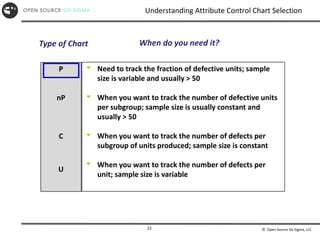
Six Sigma, LLC 22 Understanding Attribute Control Chart Selection Need to track the fraction of defective units; sample size is variable and usually > 50 When you want to track the number of defective units per subgroup; sample size is usually constant and usually > 50 When you want to track the number of defects per subgroup of units produced; sample size is constant When you want to track the number of defects per unit; sample size is variable P nP C U When do you need it? Type of Chart
22.
© Open Source
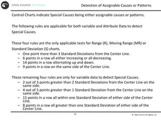
Six Sigma, LLC 23 Detection of Assignable Causes or Patterns Control Charts indicate Special Causes being either assignable causes or patterns. The following rules are applicable for both variable and Attribute Data to detect Special Causes. These four rules are the only applicable tests for Range (R), Moving Range (MR) or Standard Deviation (S) charts. – One point more than 3 Standard Deviations from the Center Line. – 6 points in a row all either increasing or all decreasing. – 14 points in a row alternating up and down. – 9 points in a row on the same side of the Center Line. These remaining four rules are only for variable data to detect Special Causes. – 2 out of 3 points greater than 2 Standard Deviations from the Center Line on the same side. – 4 out of 5 points greater than 1 Standard Deviation from the Center Line on the same side. – 15 points in a row all within one Standard Deviation of either side of the Center Line. – 8 points in a row all greater than one Standard Deviation of either side of the Center Line.
23.
© Open Source
Six Sigma, LLC 24 Recommended Special Cause Detection Rules • If implementing SPC manually without software initially the most visually obvious violations are more easily detected. SPC on manually filled charts are common place for initial use of Defect Prevention techniques. • These three rules are visually the most easily detected by personnel. – One point more than 3 Standard Deviations from the Center Line. – 6 points in a row all either increasing or all decreasing. – 15 points in a row all within one Standard Deviation of either side of the Center Line. • Dr. Shewhart working with the Western Electric Co. was credited with the following four rules referred to as Western Electric Rules. – One point more than 3 Standard Deviations from the Center Line. – 8 points in a row on the same side of the Center Line. – 2 out of 3 points greater than 2 Standard Deviations from the Center Line on the same side. – 4 out of 5 points greater than 1 Standard Deviation from the Center Line on the same side. • You might notice the Western Electric rules vary slightly. The importance is to be consistent in your organization deciding what rules you will use to detect Special Causes. • VERY few organizations use all eight rules for detecting Special Causes.
Download