SlideShare a Scribd company logo
1 of 66
Download to read offline
Statistical Process Control
© Open S ourceS ix Sigma
, LLC
LSS Green Belt v11.1 MT - Control Phase 2
Statistical Process Control
Methodology
Elements and Purpose
Special Cause Tests
Examples
Six Sigma Control Plans
Lean Controls
Welcome to Control
Statistical Process Control (SPC)
Wrap Up & Action Items
© Open S ourceS ix Sigma
, LLC
LSS Green Belt v11.1 MT - Control Phase 3
SPC Overview: Collecting Data
Population:
– An entire group of objects that have been made or
will be made containing a characteristic of interest
Sample:
– A sample is a subset of the population of interest
– The group of objects actually measured in a
statistical study
– Samples are used to estimate the true population
parameters
Population
Sample
Sample
Sample
© Open S ourceS ix Sigma
, LLC
LSS Green Belt v11.1 MT - Control Phase 4
SPC Overview: I-MR Chart
• An I-MR Chart combines a Control Chart of the average moving range with the Individuals
Chart.
• You can use Individuals Charts to track the process level and to detect the presence of
Special Causes when the sample size is one batch.
• Seeing these charts together allows you to track both the process level and process
variation at the same time providing greater sensitivity to help detect the presence of
Special Causes.
109
97
85
73
61
49
37
25
13
1
225.0
222.5
220.0
217.5
215.0
O bser vation
Individual
Value
_
X=219.89
U C L=226.12
LC L=213.67
109
97
85
73
61
49
37
25
13
1
8
6
4
2
0
O bser vation
Moving
Range
__
M R=2.341
U C L=7.649
LC L=0
I-MR Chart
© Open S ourceS ix Sigma
, LLC
LSS Green Belt v11.1 MT - Control Phase 5
SPC Overview: Xbar-R Chart
If each of your observations consists of a subgroup of data rather than just
individual measurements an Xbar-R chart provides greater sensitivity. Failure to
form rational subgroups correctly will make your Xbar-R Charts incorrect.
23
21
19
17
15
13
11
9
7
5
3
1
225
222
219
216
Sample
Sample
Mean
_
_
X=221.13
U C L=225.76
LC L=216.50
23
21
19
17
15
13
11
9
7
5
3
1
16
12
8
4
0
Sample
Sample
Range
U C L=16.97
LC L=0
_
R=8.03
Xbar-R Chart
© Open S ourceS ix Sigma
, LLC
LSS Green Belt v11.1 MT - Control Phase 6
SPC Overview: U Chart
•C Charts and U Charts are for tracking defects.
•A U Chart can do everything a C Chart can so we will just learn how
to do a U Chart. This chart counts flaws or errors (defects). One
“search area” can have more than one flaw or error.
•Search area (unit) can be practicallyanything we wish to define. We
can look for typographical errors per page, the number of paint
blemishes on a truck door or the number of bricks a mason drops in a
workday.
•You supply the number of defects on each unit inspected.
19
17
15
13
11
9
7
5
3
1
0.14
0.12
0.10
0.08
0.06
0.04
0.02
0.00
Sample
Sample
Count
Per
Unit
_
U=0.0546
UCL=0.1241
LCL=0
1
1
U Chart of Defects
© Open S ourceS ix Sigma
, LLC
LSS Green Belt v11.1 MT - Control Phase 7
SPC Overview: P Chart
•NP Charts and P Charts are for tracking defectives.
•A P Chart can do everything an NP Chart can so we will just learn
how to do a P Chart!
•Used for tracking defectives – the item is either good or bad, pass or
fail, accept or reject.
•Center Line is the proportion of “rejects” and is also your Process
Capability.
•Input to the P Chart is a series of integers — number bad, number
rejected. In addition you must supply the sample size.
19
17
15
13
11
9
7
5
3
1
0.30
0.25
0.20
0.15
Sample
Proportion
_
P=0.2038
UCL=0.2802
LCL=0.1274
P Chart of Errors
© Open S ourceS ix Sigma
, LLC
LSS Green Belt v11.1 MT - Control Phase 8
Type 1 Corrective Action = Countermeasure: improvement made to the
process which will eliminate the error condition from occurring. The defect will
never be created. This is also referred to as a long-term corrective action in the
form of Mistake Proofing or design changes.
Type 2 Corrective Action = Flag: improvement made to the process which will
detect when the error condition has occurred. This flag will shut down the
equipment so the defect will not move forward.
SPC on X’s or Y’s with fully trained operators and staff who respect the rules.
Once a chart signals a problem everyone understands the rules of SPC and
agrees to shut down for Special Cause identification. (Cpk > certain level).
Type 3 Corrective Action = Inspection: implementation of a short-term
containment which is likely to detect the defect caused by the error condition.
Containments are typically audits or 100% inspection.
SPC on X’s or Y’s with fully trained operators. The operators have been trained
and understand the rules of SPC, but management will not empower them to
stop for investigation.
S.O.P. is implemented to attempt to detect the defects. This action is not
sustainable short-term or long-term.
SPC on X’s or Y’s without proper usage = WALL PAPER.
SPC Overview: Control Methods/Effectiveness
© Open S ourceS ix Sigma
, LLC
LSS Green Belt v11.1 MT - Control Phase 9
Purpose of Statistical Process Control
Not this special cause!!
Every process has Causes of Variation known as:
– Common Cause: Natural variability
– Special Cause: Unnatural variability
• Assignable: Reason for detected Variability
• Pattern Change: Presence of trend or unusual pattern
SPC is a basic tool to monitor variation in a process.
SPC is used to detect Special Cause variation telling us the process is
“out of control”… but does NOT tell us why.
SPC gives a glimpse of ongoing process capability AND is a visual
management tool.
© Open S ourceS ix Sigma
, LLC
LSS Green Belt v11.1 MT - Control Phase 10
Elements of Control Charts
Observation
Individual
Value
28
25
22
19
16
13
10
7
4
1
60
50
40
30
20
10
0
_
X=29.06
UCL=55.24
LCL=2.87
1
Control Chart of Recycle
Developed by Dr Walter A. Shewhart of Bell Laboratories from 1924.
Graphical and visual plot of changes in the data over time.
– This is necessary for visual management of your process.
Control Charts were designed as a methodology for indicating change in
performance, either variation or Mean/Median.
Charts have a Central Line and Control Limits to detect Special Cause variation.
Process Center
(usually the Mean)
Special Cause
VariationDetected
Control Limits
© Open S ourceS ix Sigma
, LLC
LSS Green Belt v11.1 MT - Control Phase 11
Understanding the Power of SPC
Control Charts indicate when a process is “out of control” or exhibiting Special Cause
variation but NOT why!
SPC Charts incorporate upper and lower Control Limits.
– The limits are typically +/- 3  from the Center Line.
– These limits represent 99.73% of natural variability for Normal Distributions.
SPC Charts allow workers and supervision to maintain improved process performance from
Lean Six Sigma projects.
Use of SPC Charts can be applied to all processes.
– Services, manufacturing and retail are just a few industries with SPC applications.
– Caution must be taken with use of SPC for Non-normal processes.
Control Limits describe the process variability and are unrelated to customer specifications.
(Voice of the Process instead of Voice of the Customer)
– An undesirable situation is having Control Limits wider than customer specification
limits. This will exist for poorly performing processes with a Cp less than 1.0
Many SPC Charts exist and selection must be appropriate for effectiveness.
© Open S ourceS ix Sigma
, LLC
LSS Green Belt v11.1 MT - Control Phase 12
The Control Chart Cookbook
General Steps for Constructing Control Charts
1. Select characteristic (Critical “X” or CTQ) to be charted.
2. Determine the purpose of the chart.
3. Select data-collection points.
4. Establish the basis for sub-grouping (only for Y’s).
5. Select the type of Control Chart.
6. Determine the measurement method/criteria.
7. Establish the sampling interval/frequency.
8. Determine the sample size.
9. Establish the basis of calculating the Control Limits.
10. Set up the forms or software for charting data.
11. Set up the forms or software for collecting data.
12. Prepare written instructions for all phases.
13. Conduct the necessary training.
Stirred or
Shaken?
© Open S ourceS ix Sigma
, LLC
LSS Green Belt v11.1 MT - Control Phase 13
Focus of Six Sigma and the Use of SPC
To get results should we focus our behavior on the Y or X?
Y
Dependent
Output
Effect
Symptom
Monitor
X1 . . . XN
Independent
Input
Cause
Problem
Control
When we find the “vital few” X’s first
consider using SPC on the X’s to achieve
a desired Y.
Y = f(x)
© Open S ourceS ix Sigma
, LLC
LSS Green Belt v11.1 MT - Control Phase 14
Control Chart Anatomy
Common
Cause
Variation
Process is “In
Control”
Special Cause
Variation
Process is “Out
of Control”
Special Cause
Variation
Process is “Out
of Control”
Run Chart of
data points
Process Sequence/Time Scale
Lower Control
Limit
Mean
+/-
3
sigma
Upper Control
Limit
© Open S ourceS ix Sigma
, LLC
LSS Green Belt v11.1 MT - Control Phase 15
Control and Out of Control
Outlier
Outlier
68%
95%
99.7%
3
2
1
-1
-2
-3
© Open S ourceS ix Sigma
, LLC
LSS Green Belt v11.1 MT - Control Phase 16
Size of Subgroups
Typical subgroup sizes are 3-12 for variable data:
– If difficulty of gathering sample or expense of testing exists the
size, n, is smaller.
– 3, 5 and 10 are the most common size of subgroups because of
ease of calculations when SPC is done without computers.
Lot 1
Lot 2
Lot 3
Lot 4
Lot 5
Short-term studies
Long-term study
© Open S ourceS ix Sigma
, LLC
LSS Green Belt v11.1 MT - Control Phase 17
The Impact of Variation
- Natural Process
Variation as defined by
subgroup selection
- Natural Process Variation
- Different Operators
- Natural Process Variation
- Different Operators
- Supplier Source
And, of course, if two additional
sources of variation arrive we will
detect that too!
First select the spread we
will declare as the “Natural
Process Variation” so
whenever any point lands
outside these “Control
Limits” an alarm will sound
So when a second
source of variation
appears we will know!
If you base your limits on all three sources of variation, what will sound the alarm?
-UCL
-LCL
Sources of Variation
© Open S ourceS ix Sigma
, LLC
LSS Green Belt v11.1 MT - Control Phase 18
Frequency of Sampling
Sampling Frequency is a balance between the cost of sampling and
testing versus the cost of not detecting shifts in Mean or variation.
Process knowledge is an input to frequency of samples after the
subgroup size has been decided.
– If a process shifts but cannot be detected because of too
infrequent sampling the customer suffers
– If a choice is given between a large subgroup of samples
infrequently or smaller subgroups more frequently most choose to
get information more frequently.
– In some processes with automated sampling and testing frequent
sampling is easy.
If undecided as to sample frequency, sample more frequently to confirm
detection of process shifts and reduce frequency if process variation is
still detectable.
A rule of thumb also states “sample a process at least 10 times more
frequent than the frequency of ‘out of control’ conditions”.
© Open S ourceS ix Sigma
, LLC
LSS Green Belt v11.1 MT - Control Phase 19
Frequency of Sampling
Output
5
5.5
6
6.5
7
7.5
1 7 13 19 25 31 37
Sampling too little will not allow for sufficient detection of
shifts in the process because of Special Causes.
Observation
Individual
Value
13
12
11
10
9
8
7
6
5
4
3
2
1
7.5
7.0
6.5
6.0
5.5
5.0
_
X=6.1
UCL=7.385
LCL=4.815
I Chart of Sample_3
Observation
Individual
Value
7
6
5
4
3
2
1
8
7
6
5
4
_
X=6.129
UCL=8.168
LCL=4.090
I Chart of Sample_6
Observation
Individual
Value
4
3
2
1
6.6
6.4
6.2
6.0
5.8
5.6
5.4
5.2
5.0
_
X=5.85
UCL=6.559
LCL=5.141
I Chart of Sample_12
All possible samples
Sample every hour Sample 4x per shift
Sample every half hour
© Open S ourceS ix Sigma
, LLC
LSS Green Belt v11.1 MT - Control Phase 20
SPC Selection Process
Choose Appropriate
Control Chart
type
of data
type of
attribute
data
subgroup
size
I – MR
Chart
X – R
Chart
X – S
Chart
CumSum
Chart
EWMA
Chart
C Chart U Chart
NP
Chart
P Chart
type
of defect
type of
subgroups
ATTRIBUTE CONTINUOUS
DEFECTS DEFECTIVES
VARIABLE
CONSTANT CONSTANT VARIABLE
1 2-5 10+
Number of
Incidences
Incidences
per Unit
Number of
Defectives
Proportion
Defectives
Individuals
& Moving
Range
Mean &
Range
Mean &
Std. Dev.
Cumulative
Sum
Exponentially
Weighted Moving
Average
SPECIAL CASES
Sample size
© Open S ourceS ix Sigma
, LLC
LSS Green Belt v11.1 MT - Control Phase 21
Understanding Variable Control Chart Selection
Type of Chart When do you need it?
 Production is higher volume; allows process Mean and variability to be
viewed and assessed together; more sampling than with Individuals
Chart (I) and Moving Range Charts (MR) but when subgroups are
desired. Outliers can cause issues with Range (R) charts so Standard
Deviation charts (S) used instead if concerned.
 Production is low volume or cycle time to build product is long or
homogeneous sample represents entire product (batch etc.); sampling
and testing is costly so subgroups are not desired. Control limits are
wider than Xbar Charts. Used for SPC on most inputs.
 Set-up is critical, or cost of setup scrap is high. Use for outputs
 Small shift needs to be detected often because of autocorrelation of
the output results. Used only for individuals or averages of Outputs.
Infrequently used because of calculation complexity.
 Same reasons as EWMA (Exponentially Weighted Moving Range)
except the past data is as important as present data.
Average & Range
or S
(Xbar and R or
Xbar and S)
Individual and
Moving Range
Pre-Control
Exponentially
Weighted
Moving Average
Cumulative Sum
Most Common
Less Common
© Open S ourceS ix Sigma
, LLC
LSS Green Belt v11.1 MT - Control Phase 22
Understanding Attribute Control Chart Selection
 Need to track the fraction of defective units; sample
size is variable and usually > 50
 When you want to track the number of defective
units per subgroup; sample size is usually constant
and usually > 50
 When you want to track the number of defects per
subgroup of units produced; sample size is constant
 When you want to track the number of defects per
unit; sample size is variable
P
nP
C
U
When do you need it?
Type of Chart
© Open S ourceS ix Sigma
, LLC
LSS Green Belt v11.1 MT - Control Phase 23
Detection of Assignable Causes or Patterns
Control Charts indicate Special Causes being either assignable causes or patterns.
The following rules are applicable for both variable and Attribute Data to detect Special
Causes.
These four rules are the only applicable tests for Range (R), Moving Range (MR) or Standard
Deviation (S) charts.
– One point more than 3 Standard Deviations from the Center Line.
– 6 points in a row all either increasing or all decreasing.
– 14 points in a row alternating up and down.
– 9 points in a row on the same side of the center line.
These remaining four rules are only for variable data to detect Special Causes.
– 2 out of 3 points greater than 2 Standard Deviations from the Center Line on the same
side.
– 4 out of 5 points greater than 1 Standard Deviation from the Center Line on the same
side.
– 15 points in a row all within one Standard Deviation of either side of the Center Line.
– 8 points in a row all greater than one Standard Deviation of either side of the Center
Line.
© Open S ourceS ix Sigma
, LLC
LSS Green Belt v11.1 MT - Control Phase 24
Recommended Special Cause Detection Rules
• If implementing SPC manually without software initially the most visually obvious
violations are more easily detected. SPC on manually filled charts are common
place for initial use of Defect Prevention techniques.
• These three rules are visually the most easily detected by personnel.
– One point more than 3 Standard Deviations from the Center Line.
– 6 points in a row all either increasing or all decreasing.
– 15 points in a row all within one Standard Deviation of either side of the Center Line.
• Dr. Shewhart working with the Western Electric Co. was credited with the
following four rules referred to as Western Electric Rules.
– One point more than 3 Standard Deviations from the Center Line.
– 8 points in a row on the same side of the Center Line.
– 2 out of 3 points greater than 2 Standard Deviations from the Center Line on the same
side.
– 4 out of 5 points greater than 1 Standard Deviation from the Center Line on the same
side.
• You might notice the Western Electric rules vary slightly. The importance is to be
consistent in your organization deciding what rules you will use to detect Special
Causes.
• VERY few organizations use all eight rules for detecting Special Causes.
© Open S ourceS ix Sigma
, LLC
LSS Green Belt v11.1 MT - Control Phase 25
Special Cause Rule Default in MINITABTM
If a Belt is using MINITABTM she must be aware of the default
setting rules. Program defaults may be altered by:
Many experts have commented on the appropriate tests and
numbers to be used. Decide, then be consistent when
implementing.
Tools>Options>Control Charts and Quality Tools> Tests
© Open S ourceS ix Sigma
, LLC
LSS Green Belt v11.1 MT - Control Phase 26
Special Cause Test Examples
Test 1 One point beyond zone A
A
B
C
C
B
A
1
This is the MOST common Special Cause test used in SPC charts.
© Open S ourceS ix Sigma
, LLC
LSS Green Belt v11.1 MT - Control Phase 27
Special Cause Test Examples
This test is an indication of a shift in the process Mean.
Test 2 Nine points in a row on
same side of center line
A
B
C
C
B
A
2
© Open S ourceS ix Sigma
, LLC
LSS Green Belt v11.1 MT - Control Phase 28
Special Cause Test Examples
A
B
C
C
B
A
3
Test 3 Six points in a row, all
increasing or decreasing
This test is indicating a trend or gradual shift in the Mean.
© Open S ourceS ix Sigma
, LLC
LSS Green Belt v11.1 MT - Control Phase 29
Special Cause Test Examples
This test is indicating a non-random pattern.
A
B
C
C
B
A
4
Test 4 Fourteen points in a
row, alternating up and down
© Open S ourceS ix Sigma
, LLC
LSS Green Belt v11.1 MT - Control Phase 30
Special Cause Test Examples
This test is indicating a shift in the Mean or a worsening of
variation.
Test 5 Two out of three points in
a row in zone A (one side of center
line)
A
B
C
C
B
A
5
5
© Open S ourceS ix Sigma
, LLC
LSS Green Belt v11.1 MT - Control Phase 31
Special Cause Test Examples
This test is indicating a shift in the Mean or degradation of
variation.
Test 6 Four out of five points in
zone B or beyond (one side of
center line)
A
B
C
C
B
A
6
6
© Open S ourceS ix Sigma
, LLC
LSS Green Belt v11.1 MT - Control Phase 32
Special Cause Test Examples
This test is indicating a dramatic improvement of the
variation in the process.
Test 7 Fifteen points in a row in
zone C (both sides of center line)
A
B
C
C
B
A
7
© Open S ourceS ix Sigma
, LLC
LSS Green Belt v11.1 MT - Control Phase 33
Special Cause Test Examples
Test 8 Eight points in a row
beyond zone C (both sides of
center line)
A
B
C
C
B
A
8
This test is indicating a severe worsening of variation.
© Open S ourceS ix Sigma
, LLC
LSS Green Belt v11.1 MT - Control Phase 34
SPC Center Line and Control Limit Calculations
Calculate the parameters of the Individual and MR Control Charts with
the following:
Where ~
Xbar: Average of the individuals becomes the Center Line on the Individuals Chart
Xi: Individual data points
k: Number of individual data points
Ri : Moving range between individuals generally calculated using the difference between
each successive pair of readings
MRbar: The average moving range, the Center Line on the Range Chart
UCLX: Upper Control Limit on Individuals Chart
LCLX: Lower Control Limit on Individuals Chart
UCLMR: Upper Control Limit on moving range
LCLMR : Lower Control Limit on moving range (does not apply for sample sizes below 7)
E2, D3, D4: Constants that vary according to the sample size used in obtaining the moving range
k
x
X
k
1
i
i

=
=
k
R
R
M
k
i
i

=
R
M
E
X
UCL 2
x +
=
R
M
E
X
LCL 2
x −
=
R
M
D
UCL 4
MR =
R
M
D
LCL 3
MR =
Center Line Control Limits
© Open S ourceS ix Sigma
, LLC
LSS Green Belt v11.1 MT - Control Phase 35
SPC Center Line and Control Limit Calculations
Calculate the parameters of the Xbar and R Control Charts with the
following:
k
x
X
k
1
i
i

=
=
k
R
R
k
i
i

=
R
A
X
UCL 2
x +
=
R
A
X
LCL 2
x −
=
R
D
UCL 4
R =
R
D
LCL 3
R =
Center Line Control Limits
Where ~
Xi: Average of the subgroup averages, it becomes the Center Line of the Control Chart
Xi: Average of each subgroup
k: Number of subgroups
Ri : Range of each subgroup (Maximum observation – Minimum observation)
Rbar: The average range of the subgroups, the Center Line on the Range Chart
UCLX: Upper Control Limit on Average Chart
LCLX: Lower Control Limit on Average Chart
UCLR: Upper Control Limit on Range Chart
LCLR : Lower Control Limit Range Chart
A2, D3, D4: Constants that vary according to the subgroup sample size
© Open S ourceS ix Sigma
, LLC
LSS Green Belt v11.1 MT - Control Phase 36
SPC Center Line and Control Limit
Calculations
Calculate the parameters of the Xbar and S Control Charts with the
following:
Where ~
Xi: Average of the subgroup averages it becomes the Center Line of the Control Chart
Xi: Average of each subgroup
k: Number of subgroups
si : Standard Deviation of each subgroup
Sbar: The average S. D. of the subgroups, the Center Line on the S chart
UCLX: Upper Control Limit on Average Chart
LCLX: Lower Control Limit on Average Chart
UCLS: Upper Control Limit on S Chart
LCLS : Lower Control Limit S Chart
A3, B3, B4: Constants that vary according to the subgroup sample size
k
x
X
k
1
i
i

=
=
S
A
X
UCL 3
x +
=
Center Line Control Limits
S
A
X
LCL 3
x −
=
k
s
S
k
1
i
i

=
=
S
B
UCL 4
S =
S
B
LCL 3
S =
© Open S ourceS ix Sigma
, LLC
LSS Green Belt v11.1 MT - Control Phase 37
SPC Center Line and Control Limit Calculations
Calculate the parameters of the P Control Charts with the
following:
Where~
p: Average proportion defective (0.0 – 1.0)
ni: Number inspected in each subgroup
LCLp: Lower Control Limit on P Chart
UCLp: Upper Control Limit on P Chart
inspected
items
of
number
Total
items
defective
of
number
Total
p =
i
n
p
p )
1
(
3
p
UCLp
−
+
=
Center Line Control Limits
i
n
p
p )
1
(
3
p
LCLp
−
−
=
Since the Control Limits are a function
of sample size they will vary for each
sample.
© Open S ourceS ix Sigma
, LLC
LSS Green Belt v11.1 MT - Control Phase 38
SPC Center Line and Control Limit Calculations
Calculate the parameters of the nP Control Charts with the
following:
Where ~
np: Average number defective items per subgroup
ni: Number inspected in each subgroup
LCLnp: Lower Control Limit on nP chart
UCLnp: Upper Control Limit on nP chart
subgroups
of
number
Total
items
defective
of
number
Total
p
n = )
1
(
3
p
n
UCL i
np p
p
ni −
+
=
Center Line Control Limits
p)
-
p(1
n
3
p
n
LCL i
i
np −
=
Since the Control Limits AND Center Line are a
function of sample size they will vary for each
sample.
© Open S ourceS ix Sigma
, LLC
LSS Green Belt v11.1 MT - Control Phase 39
SPC Center Line and Control Limit Calculations
Calculate the parameters of the U Control Charts with the
following:
Where ~
u: Total number of defects divided by the total number of units inspected.
ni: Number inspected in each subgroup
LCLu: Lower Control Limit on U Chart.
UCLu: Upper Control Limit on U Chart.
Inspected
Units
of
number
Total
Identified
defects
of
number
Total
u =
i
n
u
3
u
UCLu +
=
Center Line Control Limits
Since the Control Limits are a function of
sample size they will vary for each sample.
i
n
u
3
u
LCLu −
=
© Open S ourceS ix Sigma
, LLC
LSS Green Belt v11.1 MT - Control Phase 40
SPC Center Line and Control Limit Calculations
Calculate the parameters of the C Control Charts with the
following:
Where ~
c: Total number of defects divided by the total number of subgroups.
LCLc: Lower Control Limit on C Chart.
UCLc: Upper Control Limit on C Chart.
subgroups
of
number
Total
defects
of
number
Total
c = c
3
c
UCLc +
=
Center Line Control Limits
c
3
c
LCLc −
=
© Open S ourceS ix Sigma
, LLC
LSS Green Belt v11.1 MT - Control Phase 41
SPC Center Line and Control Limit Calculations
Calculate the parameters of the EWMA Control Charts with the
following:
Where ~
Zt: EWMA statistic plotted on Control Chart at time t
Zt-1: EWMA statistic plotted on Control Chart at time t-1
: The weighting factor between 0 and 1 – suggest using 0.2
: Standard Deviation of historical data (pooled Standard Deviation for subgroups
– MRbar/d2 for individual observations)
Xt: Individual data point or sample averages at time t
UCL: Upper Control Limit on EWMA Chart
LCL: Lower Control Limit on EWMA Chart
n: Subgroup sample size
1
t
t
t Z
λ)
(1
X
λ
Z −
−
+
= ]
λ)
(1
)[1
λ
2
λ
(
n
σ
3
X
UCL 2t
−
−
−
+
=
Center Line Control Limits
]
λ)
(1
)[1
λ
2
λ
(
n
σ
3
X
LCL 2t
−
−
−
−
=
© Open S ourceS ix Sigma
, LLC
LSS Green Belt v11.1 MT - Control Phase 42
SPC Center Line and Control Limit Calculations
Calculate the parameters of the CUSUM control charts with
MINITABTM or other program since the calculations are even
more complicated than the EWMA charts.
Because of this complexity of formulas execution of either this or
the EWMA are not done without automation and computer
assistance.
Ah, anybody got a laptop?
© Open S ourceS ix Sigma
, LLC
LSS Green Belt v11.1 MT - Control Phase 43
Pre-Control Charts
Pre-Control Charts use limits relativeto the specification limits. This is
the first and ONLY chart wherein you will see specification limits plotted
for Statistical Process Control. This is the most basic type of chart and
unsophisticated use of process control.
Red Zones. Zone outside the
specification limits. Signals the
process is out-of-control and
should be stopped
RED Yellow Yellow Red
GREEN
0.5 0.75
0.25 1.0
0.0
Target USL
LSL
Yellow Zones. Zone between
the PC Lines and the
specification limits indicating
caution and the need to watch
the process closely
Green Zone. Zone lies
between the PC Lines, signals
the process is in control
© Open S ourceS ix Sigma
, LLC
LSS Green Belt v11.1 MT - Control Phase 44
Process Setup and Restart with Pre-Control
Qualifying Process
• To qualify a process five consecutive parts must fall within the green
zone
• The process should be qualified after tool changes,
adjustments, new operators, material changes, etc.
Monitoring Ongoing Process
• Sample two consecutive parts at predetermined frequency
– If either part is in the red, stop production and find reason for
variation
– When one part falls in the yellow zone inspect the other and:
• If the second part falls in the green zone then continue
• If the second part falls in the yellow zone on the same side
make an adjustment to the process
• If second part falls in the yellow zone on the opposite side or
in the red zone the process is out of control and should be
stopped
– If any part falls outside the specification limits or in the red zone
the process is out of control and should be stopped
© Open S ourceS ix Sigma
, LLC
LSS Green Belt v11.1 MT - Control Phase 45
Responding to Out of Control Indications
• The power of SPC is not to find out what the Center Line and Control Limits are.
• The power is to react to the Out of Control (OOC) indications with your Out of
Control Action Plans (OCAP) for the process involved. These actions are your
corrective actions to correct the output or input to achieve proper conditions.
• SPC requires immediate response to a Special Cause indication.
• SPC also requires no “sub optimizing” by those operating the process.
– Variability will increase if operators always adjust on every point if not at the
Center Line. ONLY respond when an Out of Control or Special Cause is
detected.
– Training is required to interpret the charts and response to the charts.
Observation
Individual
Value
31
28
25
22
19
16
13
10
7
4
1
40
30
20
10
0
_
X=18.38
UCL=39.76
LCL=-3.01
1
Individual SPC chart for Response Time
OCAP
If response time is too high get
additional person on phone
bank
VIOLATION:
Special Cause is indicated
© Open S ourceS ix Sigma
, LLC
LSS Green Belt v11.1 MT - Control Phase 46
AttributeSPC Example
Practical Problem: A project has been launched to get rework
reduced to less than 25% of paychecks. Rework includes
contacting a manager about overtime hours to be paid. The
project made some progress but decides they need to
implement SPC to sustain the gains and track % defective.
Please analyze the file “paycheck2.mtw” and determine the
Control Limits and Center Line.
Step 3 and 5 of the methodology is the primary focus for this
example.
– Select the appropriate Control Chart and Special Cause tests to
employ
– Calculate the Center Line and Control Limits
– Looking at the data set we see 20 weeks of data.
– The sample size is constant at 250.
– The amount of defective in the sample is in column C3.
Paycheck2.mtw
© Open S ourceS ix Sigma
, LLC
LSS Green Belt v11.1 MT - Control Phase 47
AttributeSPC Example (cont.)
© Open S ourceS ix Sigma
, LLC
LSS Green Belt v11.1 MT - Control Phase 48
AttributeSPC Example (cont.)
Notice specifications were never discussed. Let’s calculate
the Control Limits and Central Line for this example.
We will confirm what rules for Special Causes are included in
our Control Chart analysis.
© Open S ourceS ix Sigma
, LLC
LSS Green Belt v11.1 MT - Control Phase 49
AttributeSPC Example (cont.)
Remember to click on the “Options…” and “Tests” tab to
clarify the rules for detecting Special Causes.
…. Chart Options>Tests
© Open S ourceS ix Sigma
, LLC
LSS Green Belt v11.1 MT - Control Phase 50
AttributeSPC Example (cont.)
No Special Causes were detected. The average %
defective checks were 20.38%. The UCL was 28.0% and
12.7% for the LCL.
Now we must see if the next few weeks are showing
Special Cause from the results. The sample size remained
at 250 and the defective checks were 61, 64, 77.
Sample
Proportion
19
17
15
13
11
9
7
5
3
1
0.30
0.25
0.20
0.15
_
P=0.2038
UCL=0.2802
LCL=0.1274
P Chart of Empl_w_Errors
© Open S ourceS ix Sigma
, LLC
LSS Green Belt v11.1 MT - Control Phase 51
AttributeSPC Example (cont.)
Let’s continue our example:
– Step 6: Plot process X or Y on the newly created Control Chart
– Step 7: Check for Out-Of-Control (OOC) conditions after each point
– Step 8: Interpret findings, investigate Special Cause variation & make
improvements following the Out of Control Action Plan (OCAP)
Notice the new 3 weeks of data
was entered into the spreadsheet.
© Open S ourceS ix Sigma
, LLC
LSS Green Belt v11.1 MT - Control Phase 52
AttributeSPC Example (cont.)
Place the pbar from the
first chart we created in the
“Estimate” tab. This will
prevent MINITABTM from
calculating new Control
Limits which is step 9.
Sample
Proportion
23
21
19
17
15
13
11
9
7
5
3
1
0.30
0.25
0.20
0.15
_
P=0.2038
UCL=0.2802
LCL=0.1274
1
P Chart of Empl_w_Errors
…… Chart Options>Parameters
The new updated SPC
chart is shown with one
Special Cause.
© Open S ourceS ix Sigma
, LLC
LSS Green Belt v11.1 MT - Control Phase 53
AttributeSPC example (cont.)
Because of the Special Cause the process must refer to the OCAP or Out of Control Action Plan
stating what Root Causes need to be investigated and what actions are taken to get the
process back in Control.
After the corrective actions were taken wait until the next sample is taken to see if the process
has changed to not show Special Cause actions.
– If still out of control refer to the OCAP and take further action to improve the process.
DO NOT make any more changes if the process shows back in control after the next
reading.
• Even if the next reading seems higher than the Center Line! Do not cause more
variability.
If process changes are documented after this project was closed the Control Limits should be
recalculated as in step 9 of the SPC methodology.
Sample
Proportion
23
21
19
17
15
13
11
9
7
5
3
1
0.30
0.25
0.20
0.15
_
P=0.2038
UCL=0.2802
LCL=0.1274
1
P Chart of Empl_w_Errors
© Open S ourceS ix Sigma
, LLC
LSS Green Belt v11.1 MT - Control Phase 54
VariableSPC Example
Practical Problem: A job shop drills holes for its largest
customer as a final step to deliver a highly engineered
fastener. This shop uses five drill presses and gathers data
every hour with one sample from each press representing
part of the subgroup. You can assume there is insignificant
variation within the five drills and the subgroup is across the
five drills. The data is gathered in columns C3-C7.
Step 3 and 5 of the methodology is the primary focus for
this example.
– Select the appropriate Control Chart and Special Cause
tests to employ
– Calculate the Center Line and Control Limits
Holediameter.mtw
© Open S ourceS ix Sigma
, LLC
LSS Green Belt v11.1 MT - Control Phase 55
VariableSPC Example (cont.)
VARYING
VARYING
© Open S ourceS ix Sigma
, LLC
LSS Green Belt v11.1 MT - Control Phase 56
VariableSPC Example (cont.)
Specifications were never discussed. Let’s calculate the
Control Limits and Center Line for this example.
We will confirm what rules for Special Causes are included
in our Control Chart analysis.
© Open S ourceS ix Sigma
, LLC
LSS Green Belt v11.1 MT - Control Phase 57
VariableSPC Example (cont.)
Remember to click on the “Options…” and “Tests” tab to
clarify the rules for detecting Special Causes.
We will confirm what rules for Special Causes are included
in our Control Chart analysis. The top 2 of 3 were selected.
……..Xbar-R Chart Options>Tests
© Open S ourceS ix Sigma
, LLC
LSS Green Belt v11.1 MT - Control Phase 58
VariableSPC Example (cont.)
Also confirm the Rbar method is used for estimating Standard
Deviation.
Stat>Control Charts>Variable Charts for Subgroups>Xbar-R>Xbar-R Chart Options>Estimate
© Open S ourceS ix Sigma
, LLC
LSS Green Belt v11.1 MT - Control Phase 59
VariableSPC Example (cont.)
No Special Causes were detected in the Xbar Chart. The
average hole diameter was 26.33. The UCL was 33.1 and 19.6 for
the LCL.
Now we will use the Control Chart to monitor the next 2 hours and
see if we are still in control.
Sample
Sample
M
ean
46
41
36
31
26
21
16
11
6
1
35
30
25
20
_
_
X=26.33
UC L=33.07
LC L=19.59
Sample
Sample
Range
46
41
36
31
26
21
16
11
6
1
24
18
12
6
0
_
R=11.69
UC L=24.72
LC L=0
1
Xbar-R Chart of Part1, ..., Part5
© Open S ourceS ix Sigma
, LLC
LSS Green Belt v11.1 MT - Control Phase 60
VariableSPC Example (cont.)
Some more steps….
–Step 6: Plot process X or Y on the newly created Control Chart
–Step 7: Check for Out-Of-Control (OOC) conditions after each point
–Step 8: Interpret findings, investigate Special Cause variation, &
make improvements following the Out of Control Action Plan (OCAP)
© Open S ourceS ix Sigma
, LLC
LSS Green Belt v11.1 MT - Control Phase 61
VariableSPC Example (cont.)
The updated SPC Chart is shown
with no indicated Special Causes
in the Xbar Chart. The Mean, UCL
and LCL are unchanged
because of the completed
option .
……..Xbar-R Chart Options>Parameters
Sample
Sample
M
ean
51
46
41
36
31
26
21
16
11
6
1
35
30
25
20
_
_
X=26.33
UC L=33.07
LC L=19.59
Sample
Sample
Range
51
46
41
36
31
26
21
16
11
6
1
24
18
12
6
0
_
R=11.69
UC L=24.72
LC L=0
1
Xbar-R Chart of Part1, ..., Part5
© Open S ourceS ix Sigma
, LLC
LSS Green Belt v11.1 MT - Control Phase 62
VariableSPC Example (cont.)
Because of no Special Causes the process does not refer to the OCAP or Out of
Control Action Plan and NO actions are taken.
If process changes are documented after this project was closed the Control
Limits should be recalculated as in Step 9 of the SPC methodology.
Sample
Sample
M
ean
51
46
41
36
31
26
21
16
11
6
1
35
30
25
20
_
_
X=26.33
UC L=33.07
LC L=19.59
Sample
Sample
Range
51
46
41
36
31
26
21
16
11
6
1
24
18
12
6
0
_
R=11.69
UC L=24.72
LC L=0
1
Xbar-R Chart of Part1, ..., Part5
© Open S ourceS ix Sigma
, LLC
LSS Green Belt v11.1 MT - Control Phase 63
Recalculationof SPC Chart Limits
• Step 9 of the methodology refers to recalculating SPC limits.
• Processes should see improvement in variation after usage of
SPC.
• Reduction in variation or known process shift should result in
Center Line and Control Limits recalculations.
– Statistical confidence of the changes can be confirmed
with Hypothesis Testing from the Analyze Phase.
• Consider a periodic time frame for checking Control Limits
and Center Lines.
– 3, 6, 12 months are typical and dependent on resources
and priorities
– A set frequency allows for process changes to be
captured.
• Incentive to recalculate limits include avoiding false Special
Cause detection with poorly monitored processes.
• These recommendations are true for both Variable and
© Open S ourceS ix Sigma
, LLC
LSS Green Belt v11.1 MT - Control Phase 64
SPC Chart Option in MINITABTM for  Levels
This is possible with ~
Stat>Quality Charts> …..
Options>S Limits “tab”
© Open S ourceS ix Sigma
, LLC
LSS Green Belt v11.1 MT - Control Phase 65
Summary
At this point you should be able to:
• Describe the elements of an SPC Chart and the purposes of
SPC
• Understand how SPC ranks in Defect Prevention
• Describe the 13 step route or methodology of implementing a
chart
• Design subgroups if needed for SPC usage
• Determine the frequency of sampling
• Understand the Control Chart selection methodology
• Be familiar with Control Chart parameter calculations such as
UCL, LCL and the Center Line
© Open S ourceS ix Sigma
, LLC
LSS Green Belt v11.1 MT - Control Phase
Learn about IASSC Certifications and Exam options at…
http://www.iassc.org/six-sigma-certification/
IASSC Certified Lean Six Sigma Green Belt (ICGB)
The International Association for Six Sigma Certification (IASSC) is a Professional
Association dedicated to growing and enhancing the standards within the Lean Six Sigma
Community. IASSC is the only independent third-party certification body within the Lean Six
Sigma Industry that does not provide training, mentoring and coaching or consulting
services. IASSC exclusively facilitates and delivers centralized universal Lean Six Sigma
Certification Standards testing and organizational Accreditations.
The IASSC Certified Lean Six Sigma Green
Belt (ICGB) is an internationally recognized
professional who is well versed in the Lean
Six Sigma Methodology who both leads or
supports improvement projects. The Certified
Green Belt Exam, is a 3 hour 100 question
proctored exam.

More Related Content

Similar to Statistical Process Control Presentation.pdf

Control Charts in Lab and Trend Analysis
Control Charts in Lab and Trend AnalysisControl Charts in Lab and Trend Analysis
Control Charts in Lab and Trend Analysissigmatest2011
 
STATISTICAL PROCESS CONTROL(PPT).pptx
STATISTICAL PROCESS CONTROL(PPT).pptxSTATISTICAL PROCESS CONTROL(PPT).pptx
STATISTICAL PROCESS CONTROL(PPT).pptxmayankdubey99
 
Lecture 3 Statistical ProcessControl (SPC).docx
Lecture 3 Statistical ProcessControl (SPC).docxLecture 3 Statistical ProcessControl (SPC).docx
Lecture 3 Statistical ProcessControl (SPC).docxsmile790243
 
Statistical Process Control
Statistical Process ControlStatistical Process Control
Statistical Process ControlTushar Naik
 
Control estadistico de calidad
Control estadistico de calidad Control estadistico de calidad
Control estadistico de calidad ericktc
 
Control Charts: U Chart
Control Charts: U ChartControl Charts: U Chart
Control Charts: U ChartMatt Hansen
 
Statisticalqualitycontrol
StatisticalqualitycontrolStatisticalqualitycontrol
Statisticalqualitycontrolceutics1315
 
SPC Training by D&H Engineers
SPC Training by D&H EngineersSPC Training by D&H Engineers
SPC Training by D&H EngineersD&H Engineers
 
Testing for Special Cause Variation
Testing for Special Cause VariationTesting for Special Cause Variation
Testing for Special Cause VariationMatt Hansen
 
statistical process control
 statistical process control statistical process control
statistical process controlAnkitaGorhe
 
Management quality management Lec 4
Management quality management Lec 4Management quality management Lec 4
Management quality management Lec 4cairo university
 
A-guide-to-creating-and-interpreting-run-and-control-charts
A-guide-to-creating-and-interpreting-run-and-control-chartsA-guide-to-creating-and-interpreting-run-and-control-charts
A-guide-to-creating-and-interpreting-run-and-control-chartsRohitLakhotia12
 

Similar to Statistical Process Control Presentation.pdf (20)

Spc
SpcSpc
Spc
 
Control Charts in Lab and Trend Analysis
Control Charts in Lab and Trend AnalysisControl Charts in Lab and Trend Analysis
Control Charts in Lab and Trend Analysis
 
STATISTICAL PROCESS CONTROL(PPT).pptx
STATISTICAL PROCESS CONTROL(PPT).pptxSTATISTICAL PROCESS CONTROL(PPT).pptx
STATISTICAL PROCESS CONTROL(PPT).pptx
 
5. spc control charts
5. spc   control charts5. spc   control charts
5. spc control charts
 
Lecture 3 Statistical ProcessControl (SPC).docx
Lecture 3 Statistical ProcessControl (SPC).docxLecture 3 Statistical ProcessControl (SPC).docx
Lecture 3 Statistical ProcessControl (SPC).docx
 
Statistical Process Control
Statistical Process ControlStatistical Process Control
Statistical Process Control
 
Spc
SpcSpc
Spc
 
Control estadistico de calidad
Control estadistico de calidad Control estadistico de calidad
Control estadistico de calidad
 
Control Charts: U Chart
Control Charts: U ChartControl Charts: U Chart
Control Charts: U Chart
 
Statisticalqualitycontrol
StatisticalqualitycontrolStatisticalqualitycontrol
Statisticalqualitycontrol
 
Statisticalqualitycontrol
StatisticalqualitycontrolStatisticalqualitycontrol
Statisticalqualitycontrol
 
SPC Training by D&H Engineers
SPC Training by D&H EngineersSPC Training by D&H Engineers
SPC Training by D&H Engineers
 
100018718.ppt
100018718.ppt100018718.ppt
100018718.ppt
 
Testing for Special Cause Variation
Testing for Special Cause VariationTesting for Special Cause Variation
Testing for Special Cause Variation
 
statistical process control
 statistical process control statistical process control
statistical process control
 
Total Quality tools
Total Quality toolsTotal Quality tools
Total Quality tools
 
Management quality management Lec 4
Management quality management Lec 4Management quality management Lec 4
Management quality management Lec 4
 
Control charts
Control chartsControl charts
Control charts
 
Shewhart Charts for Variables
Shewhart Charts for VariablesShewhart Charts for Variables
Shewhart Charts for Variables
 
A-guide-to-creating-and-interpreting-run-and-control-charts
A-guide-to-creating-and-interpreting-run-and-control-chartsA-guide-to-creating-and-interpreting-run-and-control-charts
A-guide-to-creating-and-interpreting-run-and-control-charts
 

Recently uploaded

Personalisation of Education by AI and Big Data - Lourdes Guàrdia
Personalisation of Education by AI and Big Data - Lourdes GuàrdiaPersonalisation of Education by AI and Big Data - Lourdes Guàrdia
Personalisation of Education by AI and Big Data - Lourdes GuàrdiaEADTU
 
e-Sealing at EADTU by Kamakshi Rajagopal
e-Sealing at EADTU by Kamakshi Rajagopale-Sealing at EADTU by Kamakshi Rajagopal
e-Sealing at EADTU by Kamakshi RajagopalEADTU
 
Transparency, Recognition and the role of eSealing - Ildiko Mazar and Koen No...
Transparency, Recognition and the role of eSealing - Ildiko Mazar and Koen No...Transparency, Recognition and the role of eSealing - Ildiko Mazar and Koen No...
Transparency, Recognition and the role of eSealing - Ildiko Mazar and Koen No...EADTU
 
Stl Algorithms in C++ jjjjjjjjjjjjjjjjjj
Stl Algorithms in C++ jjjjjjjjjjjjjjjjjjStl Algorithms in C++ jjjjjjjjjjjjjjjjjj
Stl Algorithms in C++ jjjjjjjjjjjjjjjjjjMohammed Sikander
 
An overview of the various scriptures in Hinduism
An overview of the various scriptures in HinduismAn overview of the various scriptures in Hinduism
An overview of the various scriptures in HinduismDabee Kamal
 
The Story of Village Palampur Class 9 Free Study Material PDF
The Story of Village Palampur Class 9 Free Study Material PDFThe Story of Village Palampur Class 9 Free Study Material PDF
The Story of Village Palampur Class 9 Free Study Material PDFVivekanand Anglo Vedic Academy
 
SPLICE Working Group: Reusable Code Examples
SPLICE Working Group:Reusable Code ExamplesSPLICE Working Group:Reusable Code Examples
SPLICE Working Group: Reusable Code ExamplesPeter Brusilovsky
 
Improved Approval Flow in Odoo 17 Studio App
Improved Approval Flow in Odoo 17 Studio AppImproved Approval Flow in Odoo 17 Studio App
Improved Approval Flow in Odoo 17 Studio AppCeline George
 
會考英聽會考英聽會考英聽會考英聽會考英聽會考英聽會考英聽會考英聽會考英聽會考英聽
會考英聽會考英聽會考英聽會考英聽會考英聽會考英聽會考英聽會考英聽會考英聽會考英聽會考英聽會考英聽會考英聽會考英聽會考英聽會考英聽會考英聽會考英聽會考英聽會考英聽
會考英聽會考英聽會考英聽會考英聽會考英聽會考英聽會考英聽會考英聽會考英聽會考英聽中 央社
 
OSCM Unit 2_Operations Processes & Systems
OSCM Unit 2_Operations Processes & SystemsOSCM Unit 2_Operations Processes & Systems
OSCM Unit 2_Operations Processes & SystemsSandeep D Chaudhary
 
Sternal Fractures & Dislocations - EMGuidewire Radiology Reading Room
Sternal Fractures & Dislocations - EMGuidewire Radiology Reading RoomSternal Fractures & Dislocations - EMGuidewire Radiology Reading Room
Sternal Fractures & Dislocations - EMGuidewire Radiology Reading RoomSean M. Fox
 
ANTI PARKISON DRUGS.pptx
ANTI         PARKISON          DRUGS.pptxANTI         PARKISON          DRUGS.pptx
ANTI PARKISON DRUGS.pptxPoojaSen20
 
Trauma-Informed Leadership - Five Practical Principles
Trauma-Informed Leadership - Five Practical PrinciplesTrauma-Informed Leadership - Five Practical Principles
Trauma-Informed Leadership - Five Practical PrinciplesPooky Knightsmith
 
Book Review of Run For Your Life Powerpoint
Book Review of Run For Your Life PowerpointBook Review of Run For Your Life Powerpoint
Book Review of Run For Your Life Powerpoint23600690
 
Graduate Outcomes Presentation Slides - English (v3).pptx
Graduate Outcomes Presentation Slides - English (v3).pptxGraduate Outcomes Presentation Slides - English (v3).pptx
Graduate Outcomes Presentation Slides - English (v3).pptxneillewis46
 
UChicago CMSC 23320 - The Best Commit Messages of 2024
UChicago CMSC 23320 - The Best Commit Messages of 2024UChicago CMSC 23320 - The Best Commit Messages of 2024
UChicago CMSC 23320 - The Best Commit Messages of 2024Borja Sotomayor
 
An Overview of the Odoo 17 Knowledge App
An Overview of the Odoo 17 Knowledge AppAn Overview of the Odoo 17 Knowledge App
An Overview of the Odoo 17 Knowledge AppCeline George
 

Recently uploaded (20)

Personalisation of Education by AI and Big Data - Lourdes Guàrdia
Personalisation of Education by AI and Big Data - Lourdes GuàrdiaPersonalisation of Education by AI and Big Data - Lourdes Guàrdia
Personalisation of Education by AI and Big Data - Lourdes Guàrdia
 
e-Sealing at EADTU by Kamakshi Rajagopal
e-Sealing at EADTU by Kamakshi Rajagopale-Sealing at EADTU by Kamakshi Rajagopal
e-Sealing at EADTU by Kamakshi Rajagopal
 
Transparency, Recognition and the role of eSealing - Ildiko Mazar and Koen No...
Transparency, Recognition and the role of eSealing - Ildiko Mazar and Koen No...Transparency, Recognition and the role of eSealing - Ildiko Mazar and Koen No...
Transparency, Recognition and the role of eSealing - Ildiko Mazar and Koen No...
 
Stl Algorithms in C++ jjjjjjjjjjjjjjjjjj
Stl Algorithms in C++ jjjjjjjjjjjjjjjjjjStl Algorithms in C++ jjjjjjjjjjjjjjjjjj
Stl Algorithms in C++ jjjjjjjjjjjjjjjjjj
 
An overview of the various scriptures in Hinduism
An overview of the various scriptures in HinduismAn overview of the various scriptures in Hinduism
An overview of the various scriptures in Hinduism
 
The Story of Village Palampur Class 9 Free Study Material PDF
The Story of Village Palampur Class 9 Free Study Material PDFThe Story of Village Palampur Class 9 Free Study Material PDF
The Story of Village Palampur Class 9 Free Study Material PDF
 
SPLICE Working Group: Reusable Code Examples
SPLICE Working Group:Reusable Code ExamplesSPLICE Working Group:Reusable Code Examples
SPLICE Working Group: Reusable Code Examples
 
Improved Approval Flow in Odoo 17 Studio App
Improved Approval Flow in Odoo 17 Studio AppImproved Approval Flow in Odoo 17 Studio App
Improved Approval Flow in Odoo 17 Studio App
 
會考英聽會考英聽會考英聽會考英聽會考英聽會考英聽會考英聽會考英聽會考英聽會考英聽
會考英聽會考英聽會考英聽會考英聽會考英聽會考英聽會考英聽會考英聽會考英聽會考英聽會考英聽會考英聽會考英聽會考英聽會考英聽會考英聽會考英聽會考英聽會考英聽會考英聽
會考英聽會考英聽會考英聽會考英聽會考英聽會考英聽會考英聽會考英聽會考英聽會考英聽
 
OSCM Unit 2_Operations Processes & Systems
OSCM Unit 2_Operations Processes & SystemsOSCM Unit 2_Operations Processes & Systems
OSCM Unit 2_Operations Processes & Systems
 
Sternal Fractures & Dislocations - EMGuidewire Radiology Reading Room
Sternal Fractures & Dislocations - EMGuidewire Radiology Reading RoomSternal Fractures & Dislocations - EMGuidewire Radiology Reading Room
Sternal Fractures & Dislocations - EMGuidewire Radiology Reading Room
 
Supporting Newcomer Multilingual Learners
Supporting Newcomer  Multilingual LearnersSupporting Newcomer  Multilingual Learners
Supporting Newcomer Multilingual Learners
 
ANTI PARKISON DRUGS.pptx
ANTI         PARKISON          DRUGS.pptxANTI         PARKISON          DRUGS.pptx
ANTI PARKISON DRUGS.pptx
 
Trauma-Informed Leadership - Five Practical Principles
Trauma-Informed Leadership - Five Practical PrinciplesTrauma-Informed Leadership - Five Practical Principles
Trauma-Informed Leadership - Five Practical Principles
 
Book Review of Run For Your Life Powerpoint
Book Review of Run For Your Life PowerpointBook Review of Run For Your Life Powerpoint
Book Review of Run For Your Life Powerpoint
 
ESSENTIAL of (CS/IT/IS) class 07 (Networks)
ESSENTIAL of (CS/IT/IS) class 07 (Networks)ESSENTIAL of (CS/IT/IS) class 07 (Networks)
ESSENTIAL of (CS/IT/IS) class 07 (Networks)
 
Graduate Outcomes Presentation Slides - English (v3).pptx
Graduate Outcomes Presentation Slides - English (v3).pptxGraduate Outcomes Presentation Slides - English (v3).pptx
Graduate Outcomes Presentation Slides - English (v3).pptx
 
UChicago CMSC 23320 - The Best Commit Messages of 2024
UChicago CMSC 23320 - The Best Commit Messages of 2024UChicago CMSC 23320 - The Best Commit Messages of 2024
UChicago CMSC 23320 - The Best Commit Messages of 2024
 
Mattingly "AI & Prompt Design: Named Entity Recognition"
Mattingly "AI & Prompt Design: Named Entity Recognition"Mattingly "AI & Prompt Design: Named Entity Recognition"
Mattingly "AI & Prompt Design: Named Entity Recognition"
 
An Overview of the Odoo 17 Knowledge App
An Overview of the Odoo 17 Knowledge AppAn Overview of the Odoo 17 Knowledge App
An Overview of the Odoo 17 Knowledge App
 

Statistical Process Control Presentation.pdf

  • 2. © Open S ourceS ix Sigma , LLC LSS Green Belt v11.1 MT - Control Phase 2 Statistical Process Control Methodology Elements and Purpose Special Cause Tests Examples Six Sigma Control Plans Lean Controls Welcome to Control Statistical Process Control (SPC) Wrap Up & Action Items
  • 3. © Open S ourceS ix Sigma , LLC LSS Green Belt v11.1 MT - Control Phase 3 SPC Overview: Collecting Data Population: – An entire group of objects that have been made or will be made containing a characteristic of interest Sample: – A sample is a subset of the population of interest – The group of objects actually measured in a statistical study – Samples are used to estimate the true population parameters Population Sample Sample Sample
  • 4. © Open S ourceS ix Sigma , LLC LSS Green Belt v11.1 MT - Control Phase 4 SPC Overview: I-MR Chart • An I-MR Chart combines a Control Chart of the average moving range with the Individuals Chart. • You can use Individuals Charts to track the process level and to detect the presence of Special Causes when the sample size is one batch. • Seeing these charts together allows you to track both the process level and process variation at the same time providing greater sensitivity to help detect the presence of Special Causes. 109 97 85 73 61 49 37 25 13 1 225.0 222.5 220.0 217.5 215.0 O bser vation Individual Value _ X=219.89 U C L=226.12 LC L=213.67 109 97 85 73 61 49 37 25 13 1 8 6 4 2 0 O bser vation Moving Range __ M R=2.341 U C L=7.649 LC L=0 I-MR Chart
  • 5. © Open S ourceS ix Sigma , LLC LSS Green Belt v11.1 MT - Control Phase 5 SPC Overview: Xbar-R Chart If each of your observations consists of a subgroup of data rather than just individual measurements an Xbar-R chart provides greater sensitivity. Failure to form rational subgroups correctly will make your Xbar-R Charts incorrect. 23 21 19 17 15 13 11 9 7 5 3 1 225 222 219 216 Sample Sample Mean _ _ X=221.13 U C L=225.76 LC L=216.50 23 21 19 17 15 13 11 9 7 5 3 1 16 12 8 4 0 Sample Sample Range U C L=16.97 LC L=0 _ R=8.03 Xbar-R Chart
  • 6. © Open S ourceS ix Sigma , LLC LSS Green Belt v11.1 MT - Control Phase 6 SPC Overview: U Chart •C Charts and U Charts are for tracking defects. •A U Chart can do everything a C Chart can so we will just learn how to do a U Chart. This chart counts flaws or errors (defects). One “search area” can have more than one flaw or error. •Search area (unit) can be practicallyanything we wish to define. We can look for typographical errors per page, the number of paint blemishes on a truck door or the number of bricks a mason drops in a workday. •You supply the number of defects on each unit inspected. 19 17 15 13 11 9 7 5 3 1 0.14 0.12 0.10 0.08 0.06 0.04 0.02 0.00 Sample Sample Count Per Unit _ U=0.0546 UCL=0.1241 LCL=0 1 1 U Chart of Defects
  • 7. © Open S ourceS ix Sigma , LLC LSS Green Belt v11.1 MT - Control Phase 7 SPC Overview: P Chart •NP Charts and P Charts are for tracking defectives. •A P Chart can do everything an NP Chart can so we will just learn how to do a P Chart! •Used for tracking defectives – the item is either good or bad, pass or fail, accept or reject. •Center Line is the proportion of “rejects” and is also your Process Capability. •Input to the P Chart is a series of integers — number bad, number rejected. In addition you must supply the sample size. 19 17 15 13 11 9 7 5 3 1 0.30 0.25 0.20 0.15 Sample Proportion _ P=0.2038 UCL=0.2802 LCL=0.1274 P Chart of Errors
  • 8. © Open S ourceS ix Sigma , LLC LSS Green Belt v11.1 MT - Control Phase 8 Type 1 Corrective Action = Countermeasure: improvement made to the process which will eliminate the error condition from occurring. The defect will never be created. This is also referred to as a long-term corrective action in the form of Mistake Proofing or design changes. Type 2 Corrective Action = Flag: improvement made to the process which will detect when the error condition has occurred. This flag will shut down the equipment so the defect will not move forward. SPC on X’s or Y’s with fully trained operators and staff who respect the rules. Once a chart signals a problem everyone understands the rules of SPC and agrees to shut down for Special Cause identification. (Cpk > certain level). Type 3 Corrective Action = Inspection: implementation of a short-term containment which is likely to detect the defect caused by the error condition. Containments are typically audits or 100% inspection. SPC on X’s or Y’s with fully trained operators. The operators have been trained and understand the rules of SPC, but management will not empower them to stop for investigation. S.O.P. is implemented to attempt to detect the defects. This action is not sustainable short-term or long-term. SPC on X’s or Y’s without proper usage = WALL PAPER. SPC Overview: Control Methods/Effectiveness
  • 9. © Open S ourceS ix Sigma , LLC LSS Green Belt v11.1 MT - Control Phase 9 Purpose of Statistical Process Control Not this special cause!! Every process has Causes of Variation known as: – Common Cause: Natural variability – Special Cause: Unnatural variability • Assignable: Reason for detected Variability • Pattern Change: Presence of trend or unusual pattern SPC is a basic tool to monitor variation in a process. SPC is used to detect Special Cause variation telling us the process is “out of control”… but does NOT tell us why. SPC gives a glimpse of ongoing process capability AND is a visual management tool.
  • 10. © Open S ourceS ix Sigma , LLC LSS Green Belt v11.1 MT - Control Phase 10 Elements of Control Charts Observation Individual Value 28 25 22 19 16 13 10 7 4 1 60 50 40 30 20 10 0 _ X=29.06 UCL=55.24 LCL=2.87 1 Control Chart of Recycle Developed by Dr Walter A. Shewhart of Bell Laboratories from 1924. Graphical and visual plot of changes in the data over time. – This is necessary for visual management of your process. Control Charts were designed as a methodology for indicating change in performance, either variation or Mean/Median. Charts have a Central Line and Control Limits to detect Special Cause variation. Process Center (usually the Mean) Special Cause VariationDetected Control Limits
  • 11. © Open S ourceS ix Sigma , LLC LSS Green Belt v11.1 MT - Control Phase 11 Understanding the Power of SPC Control Charts indicate when a process is “out of control” or exhibiting Special Cause variation but NOT why! SPC Charts incorporate upper and lower Control Limits. – The limits are typically +/- 3  from the Center Line. – These limits represent 99.73% of natural variability for Normal Distributions. SPC Charts allow workers and supervision to maintain improved process performance from Lean Six Sigma projects. Use of SPC Charts can be applied to all processes. – Services, manufacturing and retail are just a few industries with SPC applications. – Caution must be taken with use of SPC for Non-normal processes. Control Limits describe the process variability and are unrelated to customer specifications. (Voice of the Process instead of Voice of the Customer) – An undesirable situation is having Control Limits wider than customer specification limits. This will exist for poorly performing processes with a Cp less than 1.0 Many SPC Charts exist and selection must be appropriate for effectiveness.
  • 12. © Open S ourceS ix Sigma , LLC LSS Green Belt v11.1 MT - Control Phase 12 The Control Chart Cookbook General Steps for Constructing Control Charts 1. Select characteristic (Critical “X” or CTQ) to be charted. 2. Determine the purpose of the chart. 3. Select data-collection points. 4. Establish the basis for sub-grouping (only for Y’s). 5. Select the type of Control Chart. 6. Determine the measurement method/criteria. 7. Establish the sampling interval/frequency. 8. Determine the sample size. 9. Establish the basis of calculating the Control Limits. 10. Set up the forms or software for charting data. 11. Set up the forms or software for collecting data. 12. Prepare written instructions for all phases. 13. Conduct the necessary training. Stirred or Shaken?
  • 13. © Open S ourceS ix Sigma , LLC LSS Green Belt v11.1 MT - Control Phase 13 Focus of Six Sigma and the Use of SPC To get results should we focus our behavior on the Y or X? Y Dependent Output Effect Symptom Monitor X1 . . . XN Independent Input Cause Problem Control When we find the “vital few” X’s first consider using SPC on the X’s to achieve a desired Y. Y = f(x)
  • 14. © Open S ourceS ix Sigma , LLC LSS Green Belt v11.1 MT - Control Phase 14 Control Chart Anatomy Common Cause Variation Process is “In Control” Special Cause Variation Process is “Out of Control” Special Cause Variation Process is “Out of Control” Run Chart of data points Process Sequence/Time Scale Lower Control Limit Mean +/- 3 sigma Upper Control Limit
  • 15. © Open S ourceS ix Sigma , LLC LSS Green Belt v11.1 MT - Control Phase 15 Control and Out of Control Outlier Outlier 68% 95% 99.7% 3 2 1 -1 -2 -3
  • 16. © Open S ourceS ix Sigma , LLC LSS Green Belt v11.1 MT - Control Phase 16 Size of Subgroups Typical subgroup sizes are 3-12 for variable data: – If difficulty of gathering sample or expense of testing exists the size, n, is smaller. – 3, 5 and 10 are the most common size of subgroups because of ease of calculations when SPC is done without computers. Lot 1 Lot 2 Lot 3 Lot 4 Lot 5 Short-term studies Long-term study
  • 17. © Open S ourceS ix Sigma , LLC LSS Green Belt v11.1 MT - Control Phase 17 The Impact of Variation - Natural Process Variation as defined by subgroup selection - Natural Process Variation - Different Operators - Natural Process Variation - Different Operators - Supplier Source And, of course, if two additional sources of variation arrive we will detect that too! First select the spread we will declare as the “Natural Process Variation” so whenever any point lands outside these “Control Limits” an alarm will sound So when a second source of variation appears we will know! If you base your limits on all three sources of variation, what will sound the alarm? -UCL -LCL Sources of Variation
  • 18. © Open S ourceS ix Sigma , LLC LSS Green Belt v11.1 MT - Control Phase 18 Frequency of Sampling Sampling Frequency is a balance between the cost of sampling and testing versus the cost of not detecting shifts in Mean or variation. Process knowledge is an input to frequency of samples after the subgroup size has been decided. – If a process shifts but cannot be detected because of too infrequent sampling the customer suffers – If a choice is given between a large subgroup of samples infrequently or smaller subgroups more frequently most choose to get information more frequently. – In some processes with automated sampling and testing frequent sampling is easy. If undecided as to sample frequency, sample more frequently to confirm detection of process shifts and reduce frequency if process variation is still detectable. A rule of thumb also states “sample a process at least 10 times more frequent than the frequency of ‘out of control’ conditions”.
  • 19. © Open S ourceS ix Sigma , LLC LSS Green Belt v11.1 MT - Control Phase 19 Frequency of Sampling Output 5 5.5 6 6.5 7 7.5 1 7 13 19 25 31 37 Sampling too little will not allow for sufficient detection of shifts in the process because of Special Causes. Observation Individual Value 13 12 11 10 9 8 7 6 5 4 3 2 1 7.5 7.0 6.5 6.0 5.5 5.0 _ X=6.1 UCL=7.385 LCL=4.815 I Chart of Sample_3 Observation Individual Value 7 6 5 4 3 2 1 8 7 6 5 4 _ X=6.129 UCL=8.168 LCL=4.090 I Chart of Sample_6 Observation Individual Value 4 3 2 1 6.6 6.4 6.2 6.0 5.8 5.6 5.4 5.2 5.0 _ X=5.85 UCL=6.559 LCL=5.141 I Chart of Sample_12 All possible samples Sample every hour Sample 4x per shift Sample every half hour
  • 20. © Open S ourceS ix Sigma , LLC LSS Green Belt v11.1 MT - Control Phase 20 SPC Selection Process Choose Appropriate Control Chart type of data type of attribute data subgroup size I – MR Chart X – R Chart X – S Chart CumSum Chart EWMA Chart C Chart U Chart NP Chart P Chart type of defect type of subgroups ATTRIBUTE CONTINUOUS DEFECTS DEFECTIVES VARIABLE CONSTANT CONSTANT VARIABLE 1 2-5 10+ Number of Incidences Incidences per Unit Number of Defectives Proportion Defectives Individuals & Moving Range Mean & Range Mean & Std. Dev. Cumulative Sum Exponentially Weighted Moving Average SPECIAL CASES Sample size
  • 21. © Open S ourceS ix Sigma , LLC LSS Green Belt v11.1 MT - Control Phase 21 Understanding Variable Control Chart Selection Type of Chart When do you need it?  Production is higher volume; allows process Mean and variability to be viewed and assessed together; more sampling than with Individuals Chart (I) and Moving Range Charts (MR) but when subgroups are desired. Outliers can cause issues with Range (R) charts so Standard Deviation charts (S) used instead if concerned.  Production is low volume or cycle time to build product is long or homogeneous sample represents entire product (batch etc.); sampling and testing is costly so subgroups are not desired. Control limits are wider than Xbar Charts. Used for SPC on most inputs.  Set-up is critical, or cost of setup scrap is high. Use for outputs  Small shift needs to be detected often because of autocorrelation of the output results. Used only for individuals or averages of Outputs. Infrequently used because of calculation complexity.  Same reasons as EWMA (Exponentially Weighted Moving Range) except the past data is as important as present data. Average & Range or S (Xbar and R or Xbar and S) Individual and Moving Range Pre-Control Exponentially Weighted Moving Average Cumulative Sum Most Common Less Common
  • 22. © Open S ourceS ix Sigma , LLC LSS Green Belt v11.1 MT - Control Phase 22 Understanding Attribute Control Chart Selection  Need to track the fraction of defective units; sample size is variable and usually > 50  When you want to track the number of defective units per subgroup; sample size is usually constant and usually > 50  When you want to track the number of defects per subgroup of units produced; sample size is constant  When you want to track the number of defects per unit; sample size is variable P nP C U When do you need it? Type of Chart
  • 23. © Open S ourceS ix Sigma , LLC LSS Green Belt v11.1 MT - Control Phase 23 Detection of Assignable Causes or Patterns Control Charts indicate Special Causes being either assignable causes or patterns. The following rules are applicable for both variable and Attribute Data to detect Special Causes. These four rules are the only applicable tests for Range (R), Moving Range (MR) or Standard Deviation (S) charts. – One point more than 3 Standard Deviations from the Center Line. – 6 points in a row all either increasing or all decreasing. – 14 points in a row alternating up and down. – 9 points in a row on the same side of the center line. These remaining four rules are only for variable data to detect Special Causes. – 2 out of 3 points greater than 2 Standard Deviations from the Center Line on the same side. – 4 out of 5 points greater than 1 Standard Deviation from the Center Line on the same side. – 15 points in a row all within one Standard Deviation of either side of the Center Line. – 8 points in a row all greater than one Standard Deviation of either side of the Center Line.
  • 24. © Open S ourceS ix Sigma , LLC LSS Green Belt v11.1 MT - Control Phase 24 Recommended Special Cause Detection Rules • If implementing SPC manually without software initially the most visually obvious violations are more easily detected. SPC on manually filled charts are common place for initial use of Defect Prevention techniques. • These three rules are visually the most easily detected by personnel. – One point more than 3 Standard Deviations from the Center Line. – 6 points in a row all either increasing or all decreasing. – 15 points in a row all within one Standard Deviation of either side of the Center Line. • Dr. Shewhart working with the Western Electric Co. was credited with the following four rules referred to as Western Electric Rules. – One point more than 3 Standard Deviations from the Center Line. – 8 points in a row on the same side of the Center Line. – 2 out of 3 points greater than 2 Standard Deviations from the Center Line on the same side. – 4 out of 5 points greater than 1 Standard Deviation from the Center Line on the same side. • You might notice the Western Electric rules vary slightly. The importance is to be consistent in your organization deciding what rules you will use to detect Special Causes. • VERY few organizations use all eight rules for detecting Special Causes.
  • 25. © Open S ourceS ix Sigma , LLC LSS Green Belt v11.1 MT - Control Phase 25 Special Cause Rule Default in MINITABTM If a Belt is using MINITABTM she must be aware of the default setting rules. Program defaults may be altered by: Many experts have commented on the appropriate tests and numbers to be used. Decide, then be consistent when implementing. Tools>Options>Control Charts and Quality Tools> Tests
  • 26. © Open S ourceS ix Sigma , LLC LSS Green Belt v11.1 MT - Control Phase 26 Special Cause Test Examples Test 1 One point beyond zone A A B C C B A 1 This is the MOST common Special Cause test used in SPC charts.
  • 27. © Open S ourceS ix Sigma , LLC LSS Green Belt v11.1 MT - Control Phase 27 Special Cause Test Examples This test is an indication of a shift in the process Mean. Test 2 Nine points in a row on same side of center line A B C C B A 2
  • 28. © Open S ourceS ix Sigma , LLC LSS Green Belt v11.1 MT - Control Phase 28 Special Cause Test Examples A B C C B A 3 Test 3 Six points in a row, all increasing or decreasing This test is indicating a trend or gradual shift in the Mean.
  • 29. © Open S ourceS ix Sigma , LLC LSS Green Belt v11.1 MT - Control Phase 29 Special Cause Test Examples This test is indicating a non-random pattern. A B C C B A 4 Test 4 Fourteen points in a row, alternating up and down
  • 30. © Open S ourceS ix Sigma , LLC LSS Green Belt v11.1 MT - Control Phase 30 Special Cause Test Examples This test is indicating a shift in the Mean or a worsening of variation. Test 5 Two out of three points in a row in zone A (one side of center line) A B C C B A 5 5
  • 31. © Open S ourceS ix Sigma , LLC LSS Green Belt v11.1 MT - Control Phase 31 Special Cause Test Examples This test is indicating a shift in the Mean or degradation of variation. Test 6 Four out of five points in zone B or beyond (one side of center line) A B C C B A 6 6
  • 32. © Open S ourceS ix Sigma , LLC LSS Green Belt v11.1 MT - Control Phase 32 Special Cause Test Examples This test is indicating a dramatic improvement of the variation in the process. Test 7 Fifteen points in a row in zone C (both sides of center line) A B C C B A 7
  • 33. © Open S ourceS ix Sigma , LLC LSS Green Belt v11.1 MT - Control Phase 33 Special Cause Test Examples Test 8 Eight points in a row beyond zone C (both sides of center line) A B C C B A 8 This test is indicating a severe worsening of variation.
  • 34. © Open S ourceS ix Sigma , LLC LSS Green Belt v11.1 MT - Control Phase 34 SPC Center Line and Control Limit Calculations Calculate the parameters of the Individual and MR Control Charts with the following: Where ~ Xbar: Average of the individuals becomes the Center Line on the Individuals Chart Xi: Individual data points k: Number of individual data points Ri : Moving range between individuals generally calculated using the difference between each successive pair of readings MRbar: The average moving range, the Center Line on the Range Chart UCLX: Upper Control Limit on Individuals Chart LCLX: Lower Control Limit on Individuals Chart UCLMR: Upper Control Limit on moving range LCLMR : Lower Control Limit on moving range (does not apply for sample sizes below 7) E2, D3, D4: Constants that vary according to the sample size used in obtaining the moving range k x X k 1 i i  = = k R R M k i i  = R M E X UCL 2 x + = R M E X LCL 2 x − = R M D UCL 4 MR = R M D LCL 3 MR = Center Line Control Limits
  • 35. © Open S ourceS ix Sigma , LLC LSS Green Belt v11.1 MT - Control Phase 35 SPC Center Line and Control Limit Calculations Calculate the parameters of the Xbar and R Control Charts with the following: k x X k 1 i i  = = k R R k i i  = R A X UCL 2 x + = R A X LCL 2 x − = R D UCL 4 R = R D LCL 3 R = Center Line Control Limits Where ~ Xi: Average of the subgroup averages, it becomes the Center Line of the Control Chart Xi: Average of each subgroup k: Number of subgroups Ri : Range of each subgroup (Maximum observation – Minimum observation) Rbar: The average range of the subgroups, the Center Line on the Range Chart UCLX: Upper Control Limit on Average Chart LCLX: Lower Control Limit on Average Chart UCLR: Upper Control Limit on Range Chart LCLR : Lower Control Limit Range Chart A2, D3, D4: Constants that vary according to the subgroup sample size
  • 36. © Open S ourceS ix Sigma , LLC LSS Green Belt v11.1 MT - Control Phase 36 SPC Center Line and Control Limit Calculations Calculate the parameters of the Xbar and S Control Charts with the following: Where ~ Xi: Average of the subgroup averages it becomes the Center Line of the Control Chart Xi: Average of each subgroup k: Number of subgroups si : Standard Deviation of each subgroup Sbar: The average S. D. of the subgroups, the Center Line on the S chart UCLX: Upper Control Limit on Average Chart LCLX: Lower Control Limit on Average Chart UCLS: Upper Control Limit on S Chart LCLS : Lower Control Limit S Chart A3, B3, B4: Constants that vary according to the subgroup sample size k x X k 1 i i  = = S A X UCL 3 x + = Center Line Control Limits S A X LCL 3 x − = k s S k 1 i i  = = S B UCL 4 S = S B LCL 3 S =
  • 37. © Open S ourceS ix Sigma , LLC LSS Green Belt v11.1 MT - Control Phase 37 SPC Center Line and Control Limit Calculations Calculate the parameters of the P Control Charts with the following: Where~ p: Average proportion defective (0.0 – 1.0) ni: Number inspected in each subgroup LCLp: Lower Control Limit on P Chart UCLp: Upper Control Limit on P Chart inspected items of number Total items defective of number Total p = i n p p ) 1 ( 3 p UCLp − + = Center Line Control Limits i n p p ) 1 ( 3 p LCLp − − = Since the Control Limits are a function of sample size they will vary for each sample.
  • 38. © Open S ourceS ix Sigma , LLC LSS Green Belt v11.1 MT - Control Phase 38 SPC Center Line and Control Limit Calculations Calculate the parameters of the nP Control Charts with the following: Where ~ np: Average number defective items per subgroup ni: Number inspected in each subgroup LCLnp: Lower Control Limit on nP chart UCLnp: Upper Control Limit on nP chart subgroups of number Total items defective of number Total p n = ) 1 ( 3 p n UCL i np p p ni − + = Center Line Control Limits p) - p(1 n 3 p n LCL i i np − = Since the Control Limits AND Center Line are a function of sample size they will vary for each sample.
  • 39. © Open S ourceS ix Sigma , LLC LSS Green Belt v11.1 MT - Control Phase 39 SPC Center Line and Control Limit Calculations Calculate the parameters of the U Control Charts with the following: Where ~ u: Total number of defects divided by the total number of units inspected. ni: Number inspected in each subgroup LCLu: Lower Control Limit on U Chart. UCLu: Upper Control Limit on U Chart. Inspected Units of number Total Identified defects of number Total u = i n u 3 u UCLu + = Center Line Control Limits Since the Control Limits are a function of sample size they will vary for each sample. i n u 3 u LCLu − =
  • 40. © Open S ourceS ix Sigma , LLC LSS Green Belt v11.1 MT - Control Phase 40 SPC Center Line and Control Limit Calculations Calculate the parameters of the C Control Charts with the following: Where ~ c: Total number of defects divided by the total number of subgroups. LCLc: Lower Control Limit on C Chart. UCLc: Upper Control Limit on C Chart. subgroups of number Total defects of number Total c = c 3 c UCLc + = Center Line Control Limits c 3 c LCLc − =
  • 41. © Open S ourceS ix Sigma , LLC LSS Green Belt v11.1 MT - Control Phase 41 SPC Center Line and Control Limit Calculations Calculate the parameters of the EWMA Control Charts with the following: Where ~ Zt: EWMA statistic plotted on Control Chart at time t Zt-1: EWMA statistic plotted on Control Chart at time t-1 : The weighting factor between 0 and 1 – suggest using 0.2 : Standard Deviation of historical data (pooled Standard Deviation for subgroups – MRbar/d2 for individual observations) Xt: Individual data point or sample averages at time t UCL: Upper Control Limit on EWMA Chart LCL: Lower Control Limit on EWMA Chart n: Subgroup sample size 1 t t t Z λ) (1 X λ Z − − + = ] λ) (1 )[1 λ 2 λ ( n σ 3 X UCL 2t − − − + = Center Line Control Limits ] λ) (1 )[1 λ 2 λ ( n σ 3 X LCL 2t − − − − =
  • 42. © Open S ourceS ix Sigma , LLC LSS Green Belt v11.1 MT - Control Phase 42 SPC Center Line and Control Limit Calculations Calculate the parameters of the CUSUM control charts with MINITABTM or other program since the calculations are even more complicated than the EWMA charts. Because of this complexity of formulas execution of either this or the EWMA are not done without automation and computer assistance. Ah, anybody got a laptop?
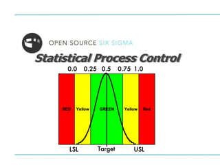
  • 43. © Open S ourceS ix Sigma , LLC LSS Green Belt v11.1 MT - Control Phase 43 Pre-Control Charts Pre-Control Charts use limits relativeto the specification limits. This is the first and ONLY chart wherein you will see specification limits plotted for Statistical Process Control. This is the most basic type of chart and unsophisticated use of process control. Red Zones. Zone outside the specification limits. Signals the process is out-of-control and should be stopped RED Yellow Yellow Red GREEN 0.5 0.75 0.25 1.0 0.0 Target USL LSL Yellow Zones. Zone between the PC Lines and the specification limits indicating caution and the need to watch the process closely Green Zone. Zone lies between the PC Lines, signals the process is in control
  • 44. © Open S ourceS ix Sigma , LLC LSS Green Belt v11.1 MT - Control Phase 44 Process Setup and Restart with Pre-Control Qualifying Process • To qualify a process five consecutive parts must fall within the green zone • The process should be qualified after tool changes, adjustments, new operators, material changes, etc. Monitoring Ongoing Process • Sample two consecutive parts at predetermined frequency – If either part is in the red, stop production and find reason for variation – When one part falls in the yellow zone inspect the other and: • If the second part falls in the green zone then continue • If the second part falls in the yellow zone on the same side make an adjustment to the process • If second part falls in the yellow zone on the opposite side or in the red zone the process is out of control and should be stopped – If any part falls outside the specification limits or in the red zone the process is out of control and should be stopped
  • 45. © Open S ourceS ix Sigma , LLC LSS Green Belt v11.1 MT - Control Phase 45 Responding to Out of Control Indications • The power of SPC is not to find out what the Center Line and Control Limits are. • The power is to react to the Out of Control (OOC) indications with your Out of Control Action Plans (OCAP) for the process involved. These actions are your corrective actions to correct the output or input to achieve proper conditions. • SPC requires immediate response to a Special Cause indication. • SPC also requires no “sub optimizing” by those operating the process. – Variability will increase if operators always adjust on every point if not at the Center Line. ONLY respond when an Out of Control or Special Cause is detected. – Training is required to interpret the charts and response to the charts. Observation Individual Value 31 28 25 22 19 16 13 10 7 4 1 40 30 20 10 0 _ X=18.38 UCL=39.76 LCL=-3.01 1 Individual SPC chart for Response Time OCAP If response time is too high get additional person on phone bank VIOLATION: Special Cause is indicated
  • 46. © Open S ourceS ix Sigma , LLC LSS Green Belt v11.1 MT - Control Phase 46 AttributeSPC Example Practical Problem: A project has been launched to get rework reduced to less than 25% of paychecks. Rework includes contacting a manager about overtime hours to be paid. The project made some progress but decides they need to implement SPC to sustain the gains and track % defective. Please analyze the file “paycheck2.mtw” and determine the Control Limits and Center Line. Step 3 and 5 of the methodology is the primary focus for this example. – Select the appropriate Control Chart and Special Cause tests to employ – Calculate the Center Line and Control Limits – Looking at the data set we see 20 weeks of data. – The sample size is constant at 250. – The amount of defective in the sample is in column C3. Paycheck2.mtw
  • 47. © Open S ourceS ix Sigma , LLC LSS Green Belt v11.1 MT - Control Phase 47 AttributeSPC Example (cont.)
  • 48. © Open S ourceS ix Sigma , LLC LSS Green Belt v11.1 MT - Control Phase 48 AttributeSPC Example (cont.) Notice specifications were never discussed. Let’s calculate the Control Limits and Central Line for this example. We will confirm what rules for Special Causes are included in our Control Chart analysis.
  • 49. © Open S ourceS ix Sigma , LLC LSS Green Belt v11.1 MT - Control Phase 49 AttributeSPC Example (cont.) Remember to click on the “Options…” and “Tests” tab to clarify the rules for detecting Special Causes. …. Chart Options>Tests
  • 50. © Open S ourceS ix Sigma , LLC LSS Green Belt v11.1 MT - Control Phase 50 AttributeSPC Example (cont.) No Special Causes were detected. The average % defective checks were 20.38%. The UCL was 28.0% and 12.7% for the LCL. Now we must see if the next few weeks are showing Special Cause from the results. The sample size remained at 250 and the defective checks were 61, 64, 77. Sample Proportion 19 17 15 13 11 9 7 5 3 1 0.30 0.25 0.20 0.15 _ P=0.2038 UCL=0.2802 LCL=0.1274 P Chart of Empl_w_Errors
  • 51. © Open S ourceS ix Sigma , LLC LSS Green Belt v11.1 MT - Control Phase 51 AttributeSPC Example (cont.) Let’s continue our example: – Step 6: Plot process X or Y on the newly created Control Chart – Step 7: Check for Out-Of-Control (OOC) conditions after each point – Step 8: Interpret findings, investigate Special Cause variation & make improvements following the Out of Control Action Plan (OCAP) Notice the new 3 weeks of data was entered into the spreadsheet.
  • 52. © Open S ourceS ix Sigma , LLC LSS Green Belt v11.1 MT - Control Phase 52 AttributeSPC Example (cont.) Place the pbar from the first chart we created in the “Estimate” tab. This will prevent MINITABTM from calculating new Control Limits which is step 9. Sample Proportion 23 21 19 17 15 13 11 9 7 5 3 1 0.30 0.25 0.20 0.15 _ P=0.2038 UCL=0.2802 LCL=0.1274 1 P Chart of Empl_w_Errors …… Chart Options>Parameters The new updated SPC chart is shown with one Special Cause.
  • 53. © Open S ourceS ix Sigma , LLC LSS Green Belt v11.1 MT - Control Phase 53 AttributeSPC example (cont.) Because of the Special Cause the process must refer to the OCAP or Out of Control Action Plan stating what Root Causes need to be investigated and what actions are taken to get the process back in Control. After the corrective actions were taken wait until the next sample is taken to see if the process has changed to not show Special Cause actions. – If still out of control refer to the OCAP and take further action to improve the process. DO NOT make any more changes if the process shows back in control after the next reading. • Even if the next reading seems higher than the Center Line! Do not cause more variability. If process changes are documented after this project was closed the Control Limits should be recalculated as in step 9 of the SPC methodology. Sample Proportion 23 21 19 17 15 13 11 9 7 5 3 1 0.30 0.25 0.20 0.15 _ P=0.2038 UCL=0.2802 LCL=0.1274 1 P Chart of Empl_w_Errors
  • 54. © Open S ourceS ix Sigma , LLC LSS Green Belt v11.1 MT - Control Phase 54 VariableSPC Example Practical Problem: A job shop drills holes for its largest customer as a final step to deliver a highly engineered fastener. This shop uses five drill presses and gathers data every hour with one sample from each press representing part of the subgroup. You can assume there is insignificant variation within the five drills and the subgroup is across the five drills. The data is gathered in columns C3-C7. Step 3 and 5 of the methodology is the primary focus for this example. – Select the appropriate Control Chart and Special Cause tests to employ – Calculate the Center Line and Control Limits Holediameter.mtw
  • 55. © Open S ourceS ix Sigma , LLC LSS Green Belt v11.1 MT - Control Phase 55 VariableSPC Example (cont.) VARYING VARYING
  • 56. © Open S ourceS ix Sigma , LLC LSS Green Belt v11.1 MT - Control Phase 56 VariableSPC Example (cont.) Specifications were never discussed. Let’s calculate the Control Limits and Center Line for this example. We will confirm what rules for Special Causes are included in our Control Chart analysis.
  • 57. © Open S ourceS ix Sigma , LLC LSS Green Belt v11.1 MT - Control Phase 57 VariableSPC Example (cont.) Remember to click on the “Options…” and “Tests” tab to clarify the rules for detecting Special Causes. We will confirm what rules for Special Causes are included in our Control Chart analysis. The top 2 of 3 were selected. ……..Xbar-R Chart Options>Tests
  • 58. © Open S ourceS ix Sigma , LLC LSS Green Belt v11.1 MT - Control Phase 58 VariableSPC Example (cont.) Also confirm the Rbar method is used for estimating Standard Deviation. Stat>Control Charts>Variable Charts for Subgroups>Xbar-R>Xbar-R Chart Options>Estimate
  • 59. © Open S ourceS ix Sigma , LLC LSS Green Belt v11.1 MT - Control Phase 59 VariableSPC Example (cont.) No Special Causes were detected in the Xbar Chart. The average hole diameter was 26.33. The UCL was 33.1 and 19.6 for the LCL. Now we will use the Control Chart to monitor the next 2 hours and see if we are still in control. Sample Sample M ean 46 41 36 31 26 21 16 11 6 1 35 30 25 20 _ _ X=26.33 UC L=33.07 LC L=19.59 Sample Sample Range 46 41 36 31 26 21 16 11 6 1 24 18 12 6 0 _ R=11.69 UC L=24.72 LC L=0 1 Xbar-R Chart of Part1, ..., Part5
  • 60. © Open S ourceS ix Sigma , LLC LSS Green Belt v11.1 MT - Control Phase 60 VariableSPC Example (cont.) Some more steps…. –Step 6: Plot process X or Y on the newly created Control Chart –Step 7: Check for Out-Of-Control (OOC) conditions after each point –Step 8: Interpret findings, investigate Special Cause variation, & make improvements following the Out of Control Action Plan (OCAP)
  • 61. © Open S ourceS ix Sigma , LLC LSS Green Belt v11.1 MT - Control Phase 61 VariableSPC Example (cont.) The updated SPC Chart is shown with no indicated Special Causes in the Xbar Chart. The Mean, UCL and LCL are unchanged because of the completed option . ……..Xbar-R Chart Options>Parameters Sample Sample M ean 51 46 41 36 31 26 21 16 11 6 1 35 30 25 20 _ _ X=26.33 UC L=33.07 LC L=19.59 Sample Sample Range 51 46 41 36 31 26 21 16 11 6 1 24 18 12 6 0 _ R=11.69 UC L=24.72 LC L=0 1 Xbar-R Chart of Part1, ..., Part5
  • 62. © Open S ourceS ix Sigma , LLC LSS Green Belt v11.1 MT - Control Phase 62 VariableSPC Example (cont.) Because of no Special Causes the process does not refer to the OCAP or Out of Control Action Plan and NO actions are taken. If process changes are documented after this project was closed the Control Limits should be recalculated as in Step 9 of the SPC methodology. Sample Sample M ean 51 46 41 36 31 26 21 16 11 6 1 35 30 25 20 _ _ X=26.33 UC L=33.07 LC L=19.59 Sample Sample Range 51 46 41 36 31 26 21 16 11 6 1 24 18 12 6 0 _ R=11.69 UC L=24.72 LC L=0 1 Xbar-R Chart of Part1, ..., Part5
  • 63. © Open S ourceS ix Sigma , LLC LSS Green Belt v11.1 MT - Control Phase 63 Recalculationof SPC Chart Limits • Step 9 of the methodology refers to recalculating SPC limits. • Processes should see improvement in variation after usage of SPC. • Reduction in variation or known process shift should result in Center Line and Control Limits recalculations. – Statistical confidence of the changes can be confirmed with Hypothesis Testing from the Analyze Phase. • Consider a periodic time frame for checking Control Limits and Center Lines. – 3, 6, 12 months are typical and dependent on resources and priorities – A set frequency allows for process changes to be captured. • Incentive to recalculate limits include avoiding false Special Cause detection with poorly monitored processes. • These recommendations are true for both Variable and
  • 64. © Open S ourceS ix Sigma , LLC LSS Green Belt v11.1 MT - Control Phase 64 SPC Chart Option in MINITABTM for  Levels This is possible with ~ Stat>Quality Charts> ….. Options>S Limits “tab”
  • 65. © Open S ourceS ix Sigma , LLC LSS Green Belt v11.1 MT - Control Phase 65 Summary At this point you should be able to: • Describe the elements of an SPC Chart and the purposes of SPC • Understand how SPC ranks in Defect Prevention • Describe the 13 step route or methodology of implementing a chart • Design subgroups if needed for SPC usage • Determine the frequency of sampling • Understand the Control Chart selection methodology • Be familiar with Control Chart parameter calculations such as UCL, LCL and the Center Line
  • 66. © Open S ourceS ix Sigma , LLC LSS Green Belt v11.1 MT - Control Phase Learn about IASSC Certifications and Exam options at… http://www.iassc.org/six-sigma-certification/ IASSC Certified Lean Six Sigma Green Belt (ICGB) The International Association for Six Sigma Certification (IASSC) is a Professional Association dedicated to growing and enhancing the standards within the Lean Six Sigma Community. IASSC is the only independent third-party certification body within the Lean Six Sigma Industry that does not provide training, mentoring and coaching or consulting services. IASSC exclusively facilitates and delivers centralized universal Lean Six Sigma Certification Standards testing and organizational Accreditations. The IASSC Certified Lean Six Sigma Green Belt (ICGB) is an internationally recognized professional who is well versed in the Lean Six Sigma Methodology who both leads or supports improvement projects. The Certified Green Belt Exam, is a 3 hour 100 question proctored exam.