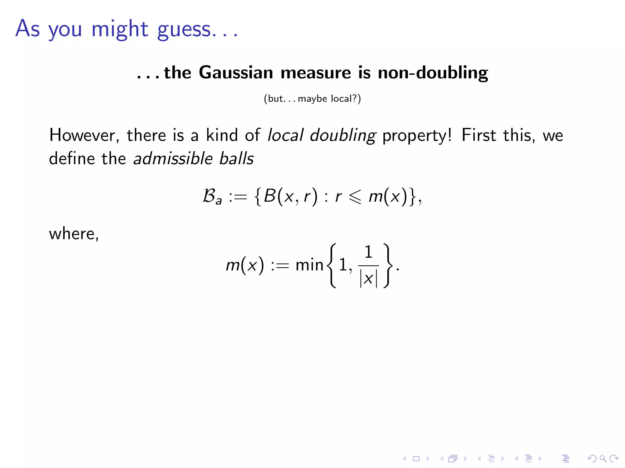
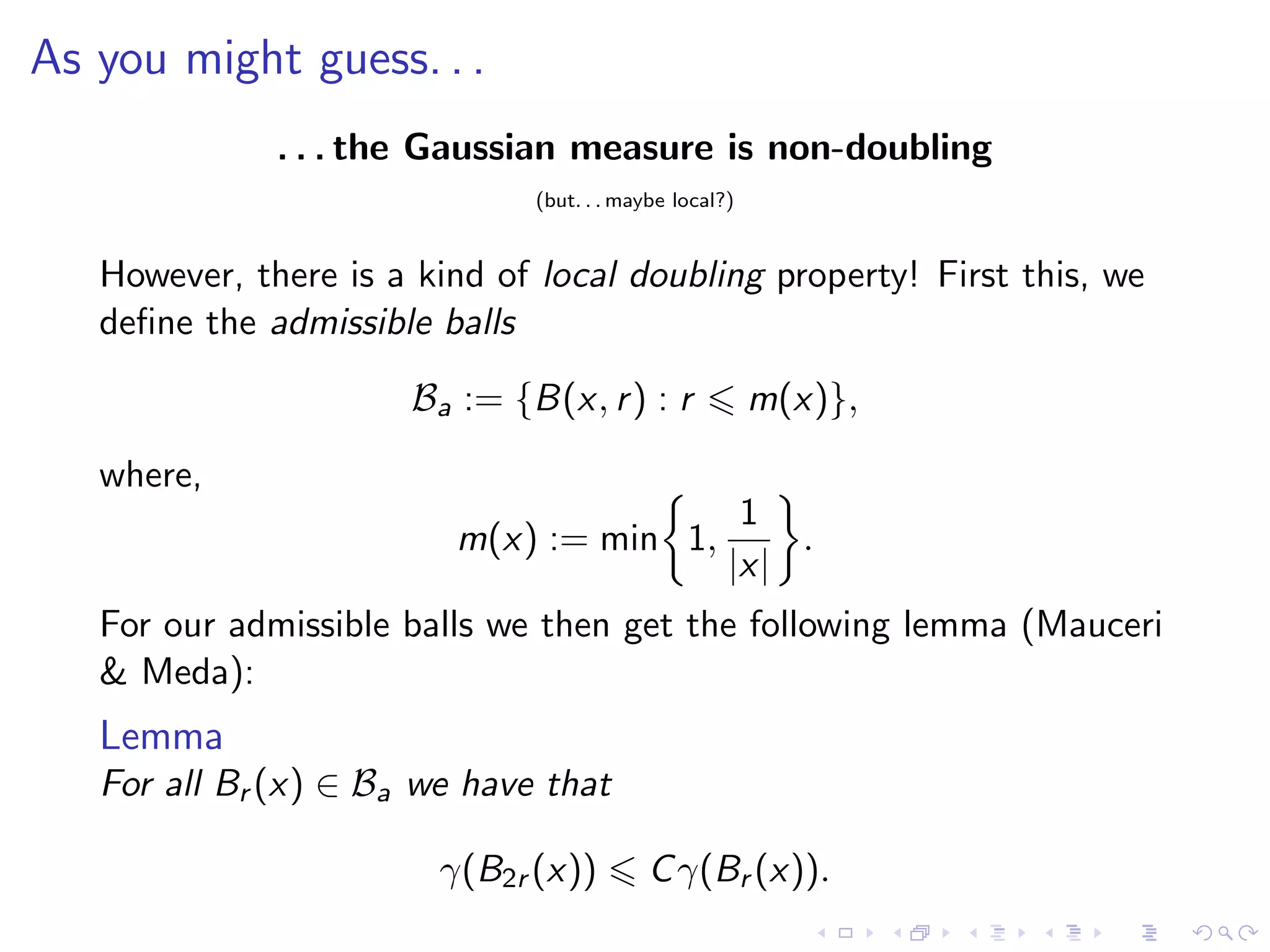
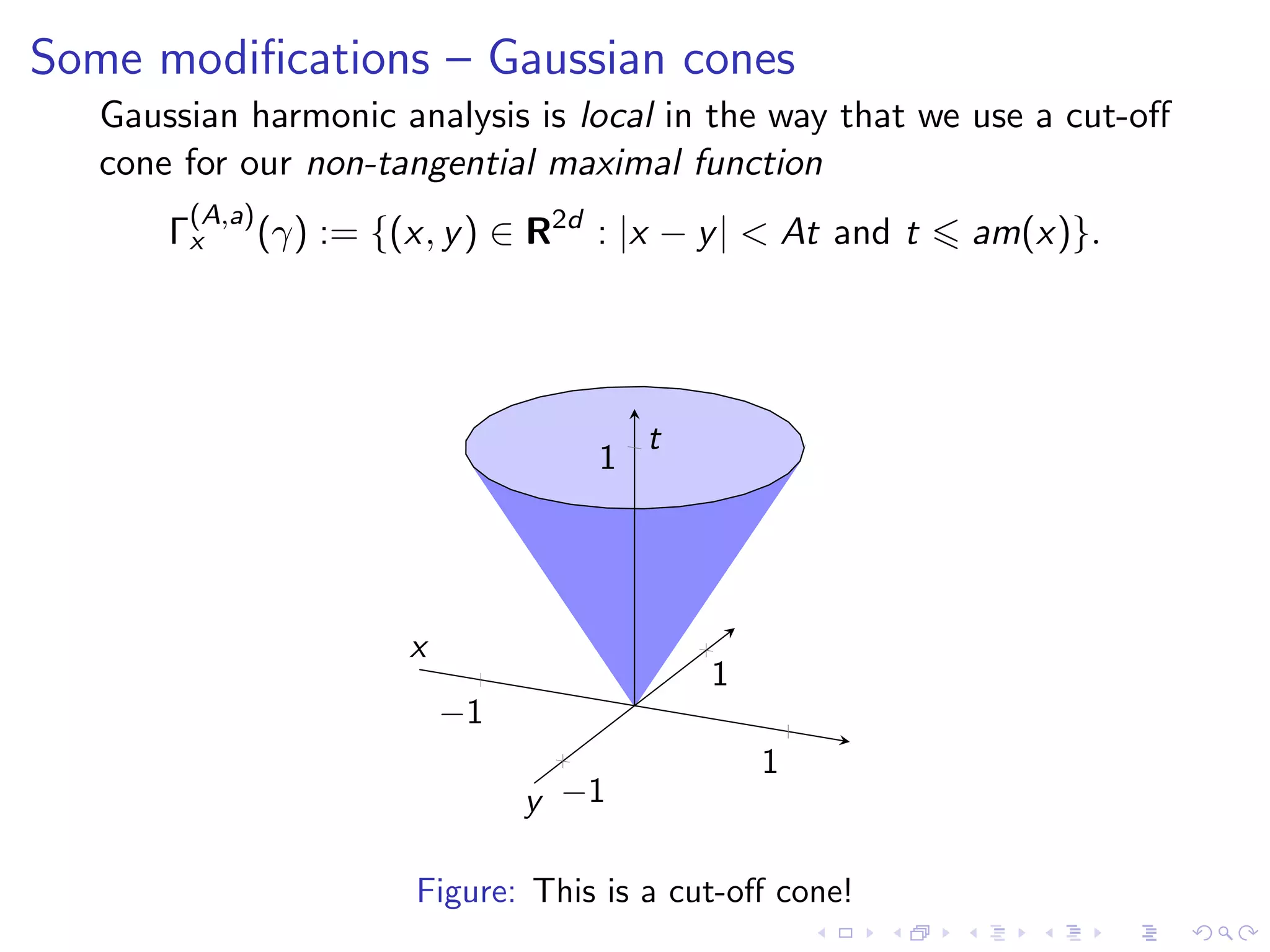
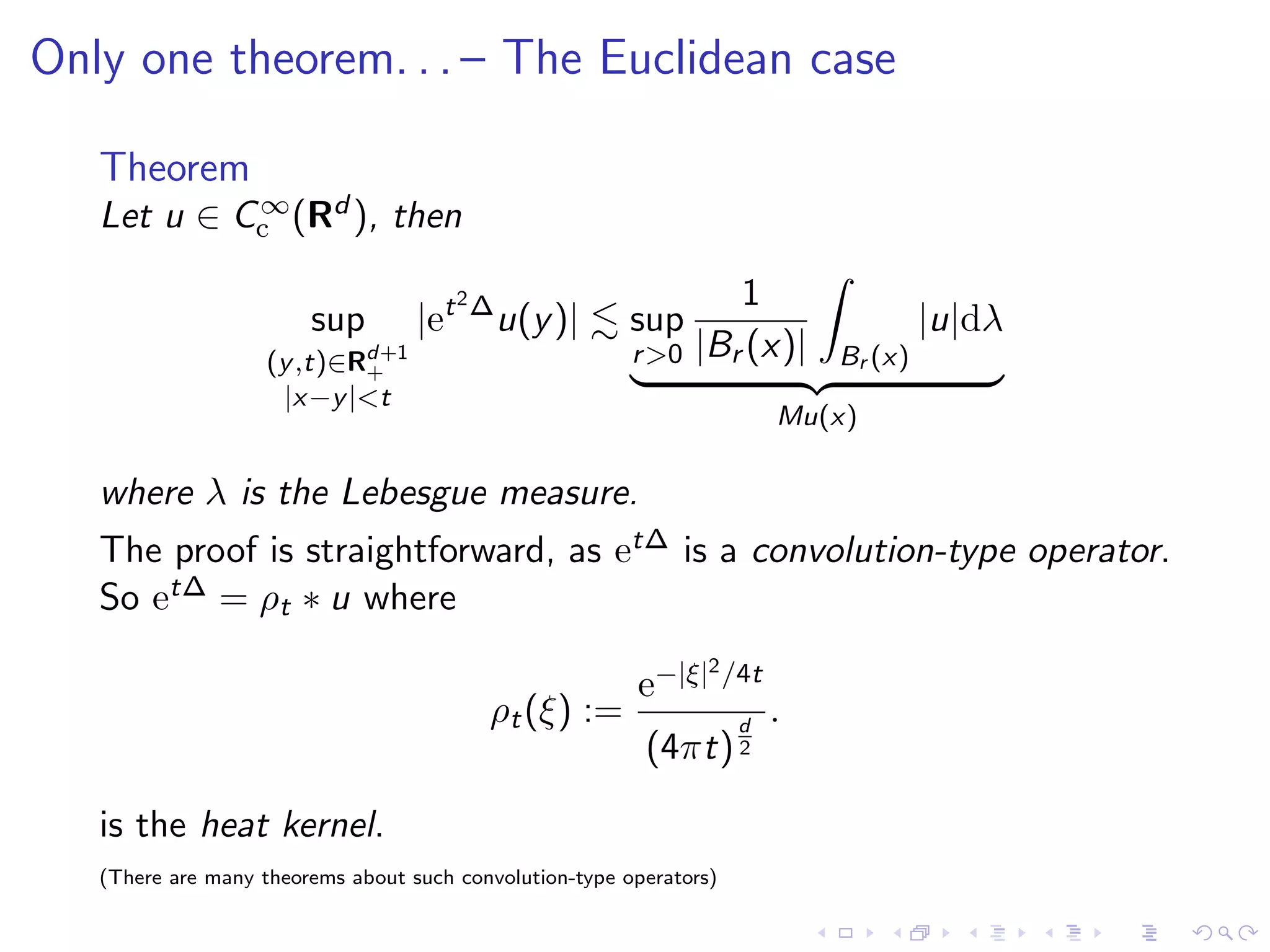
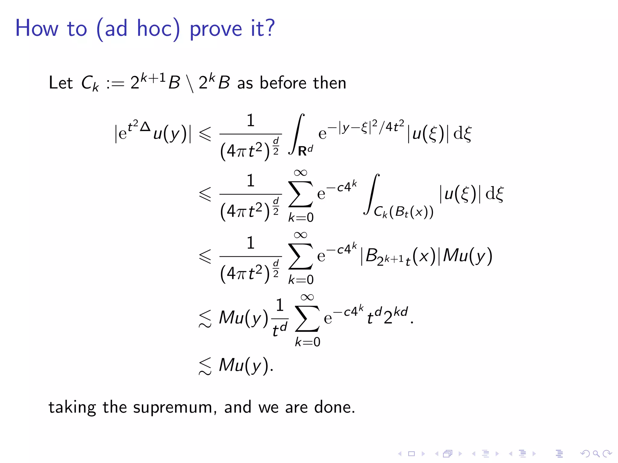
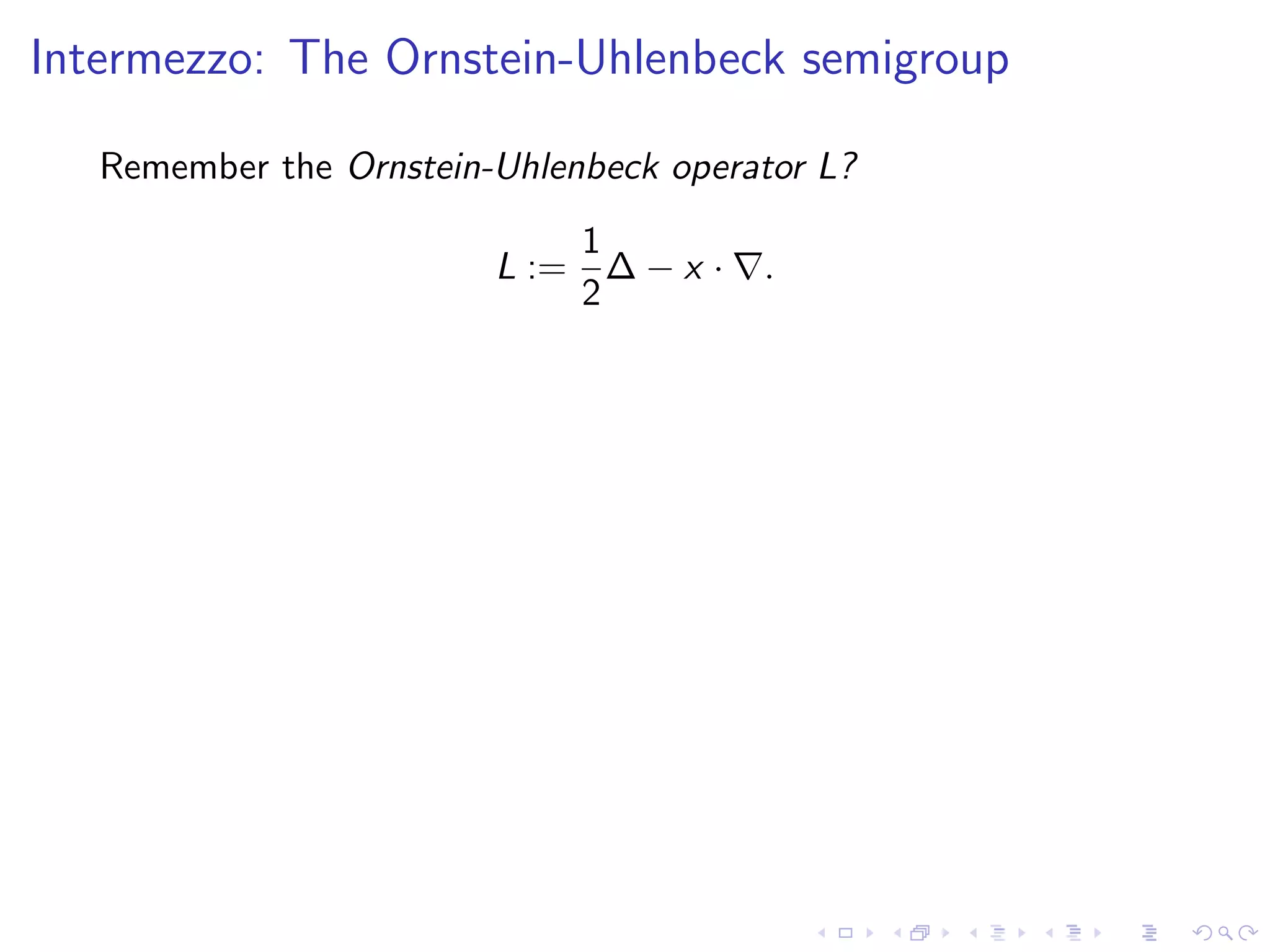
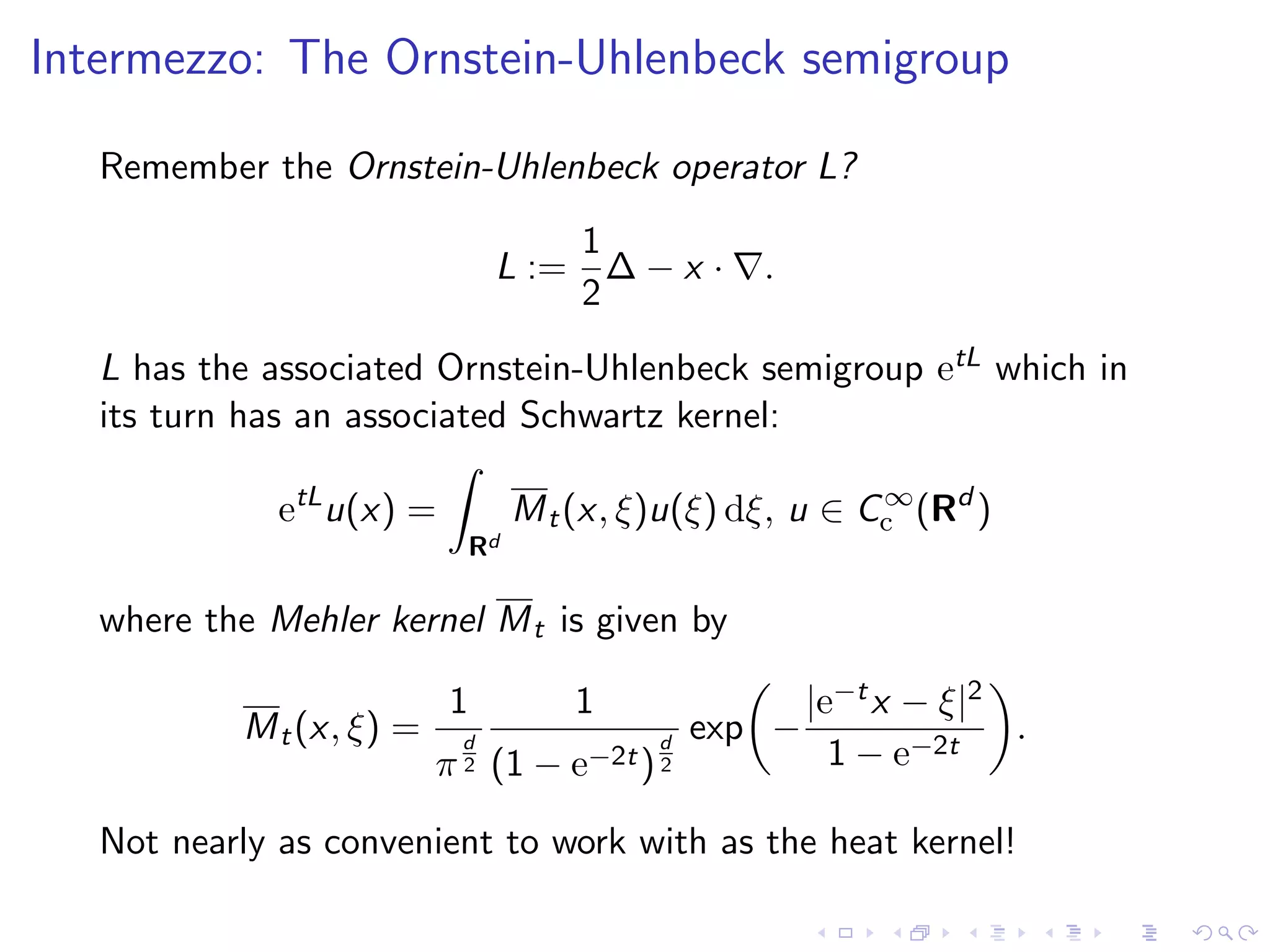
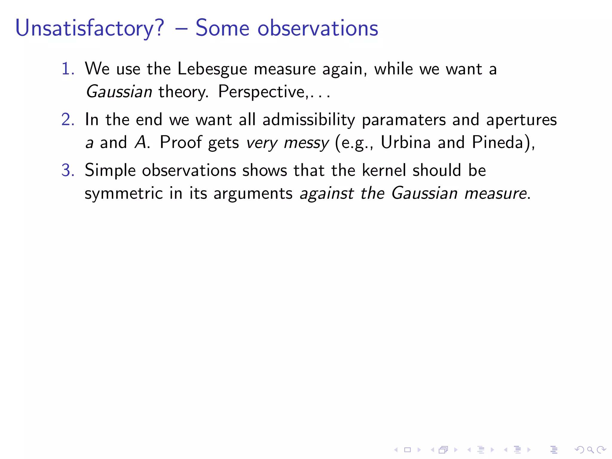
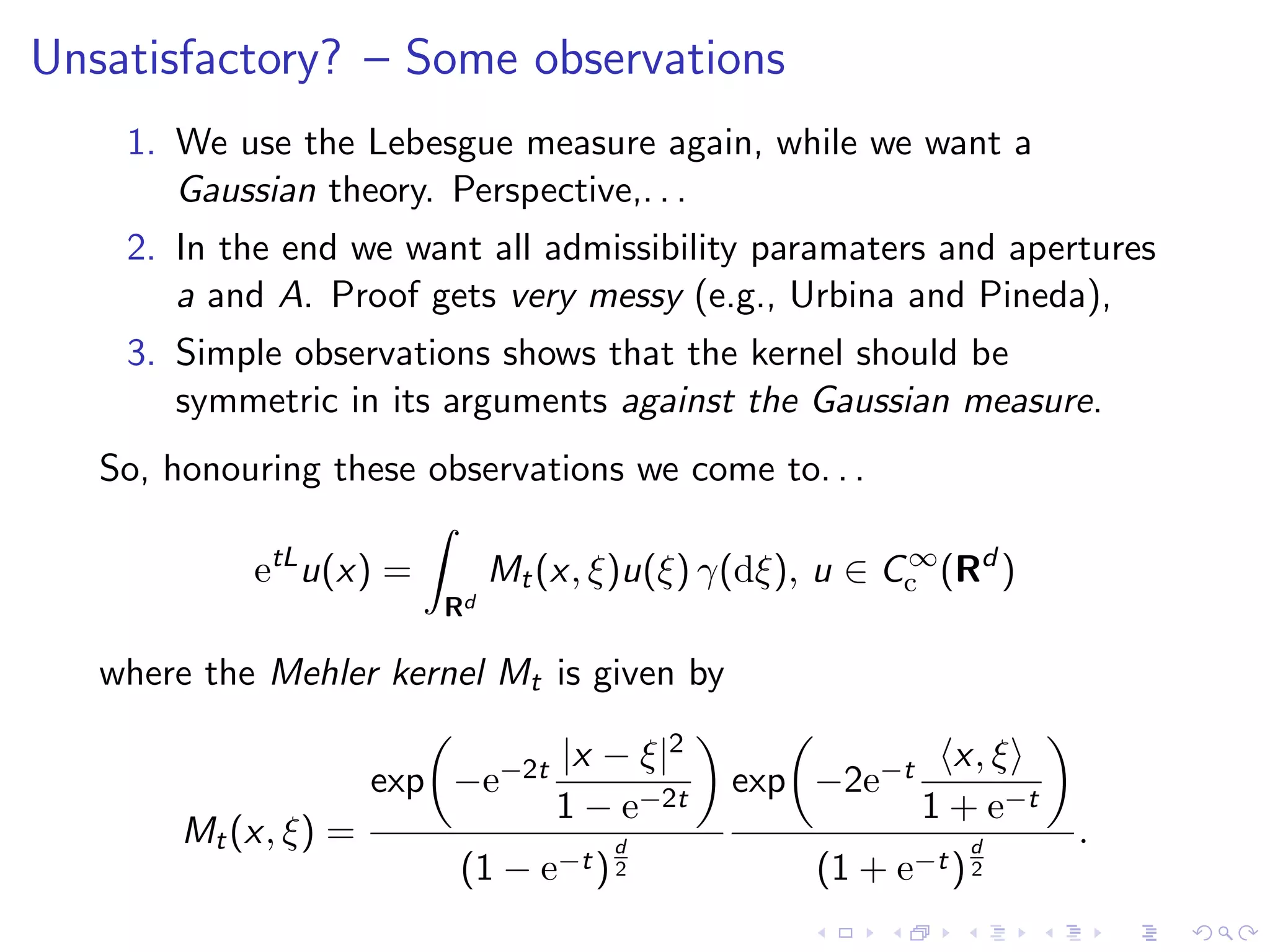
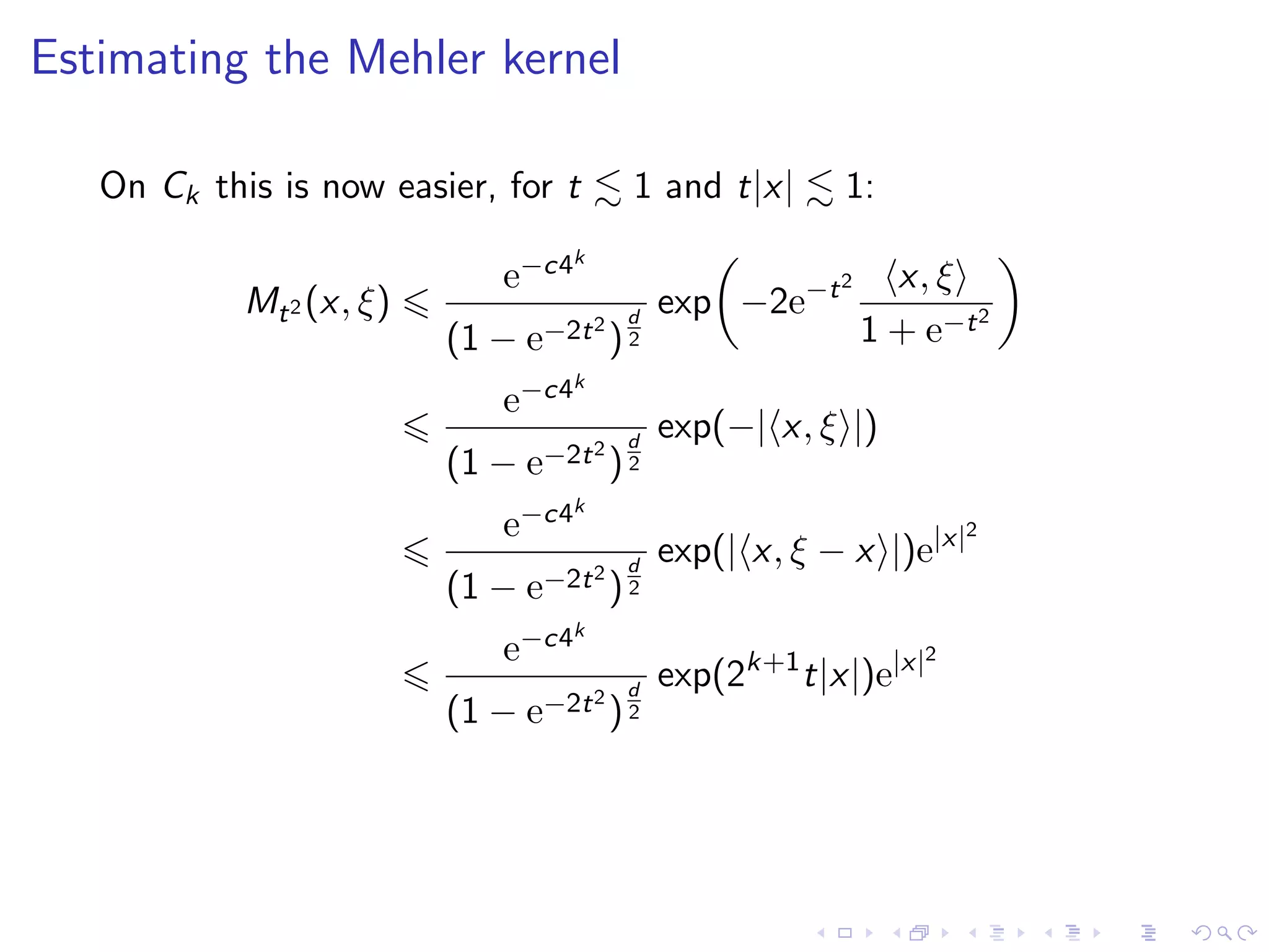
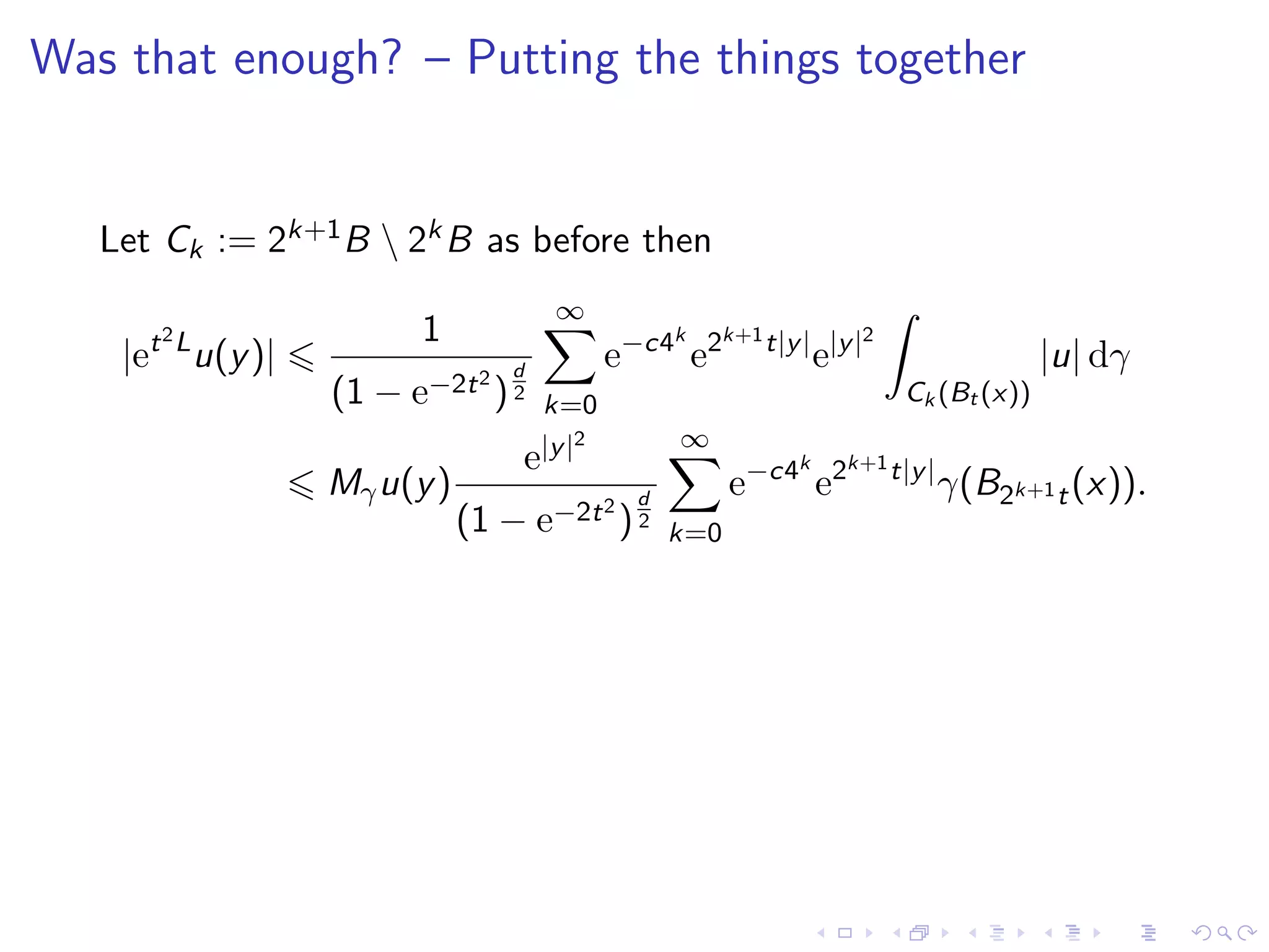
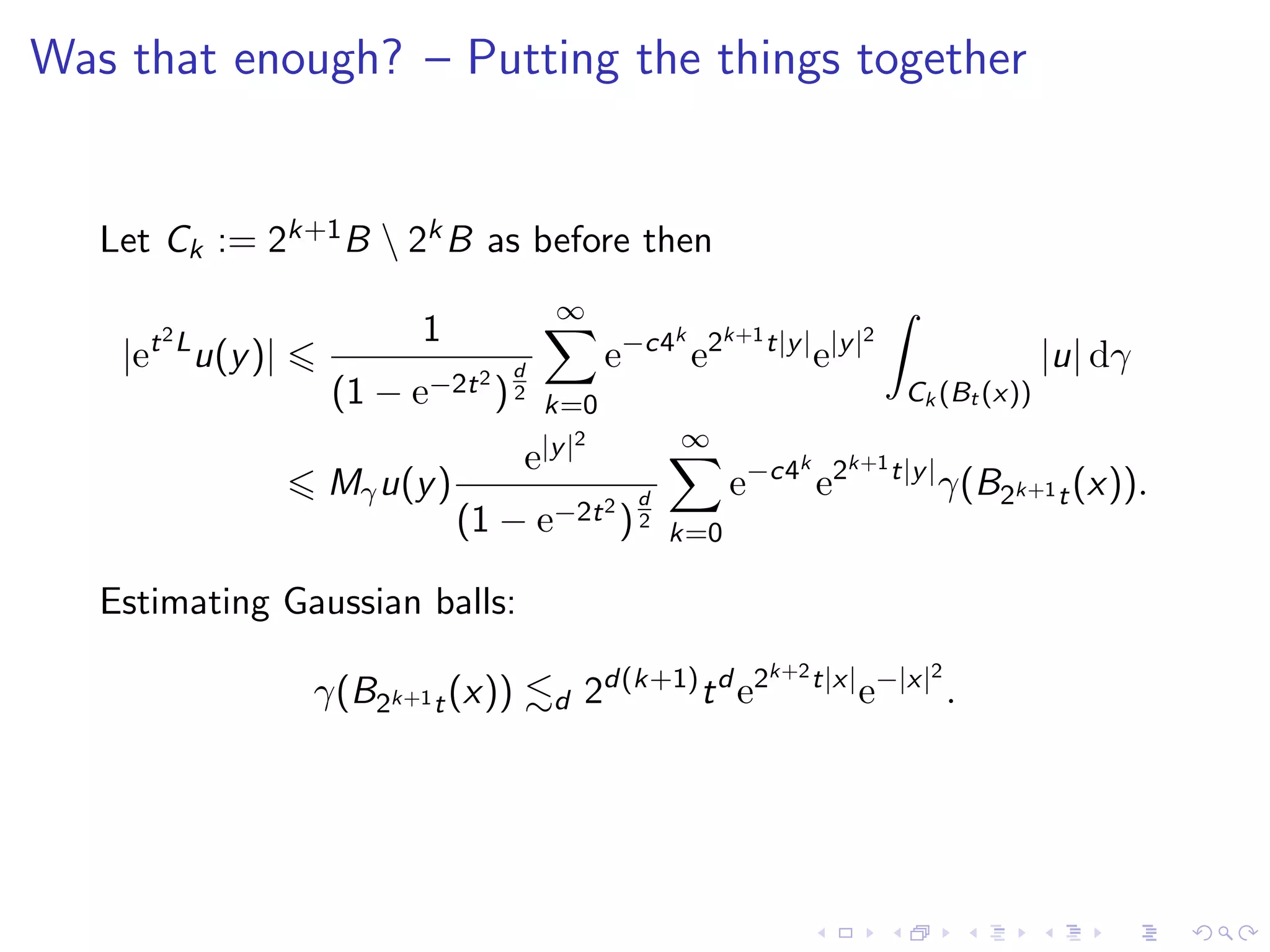
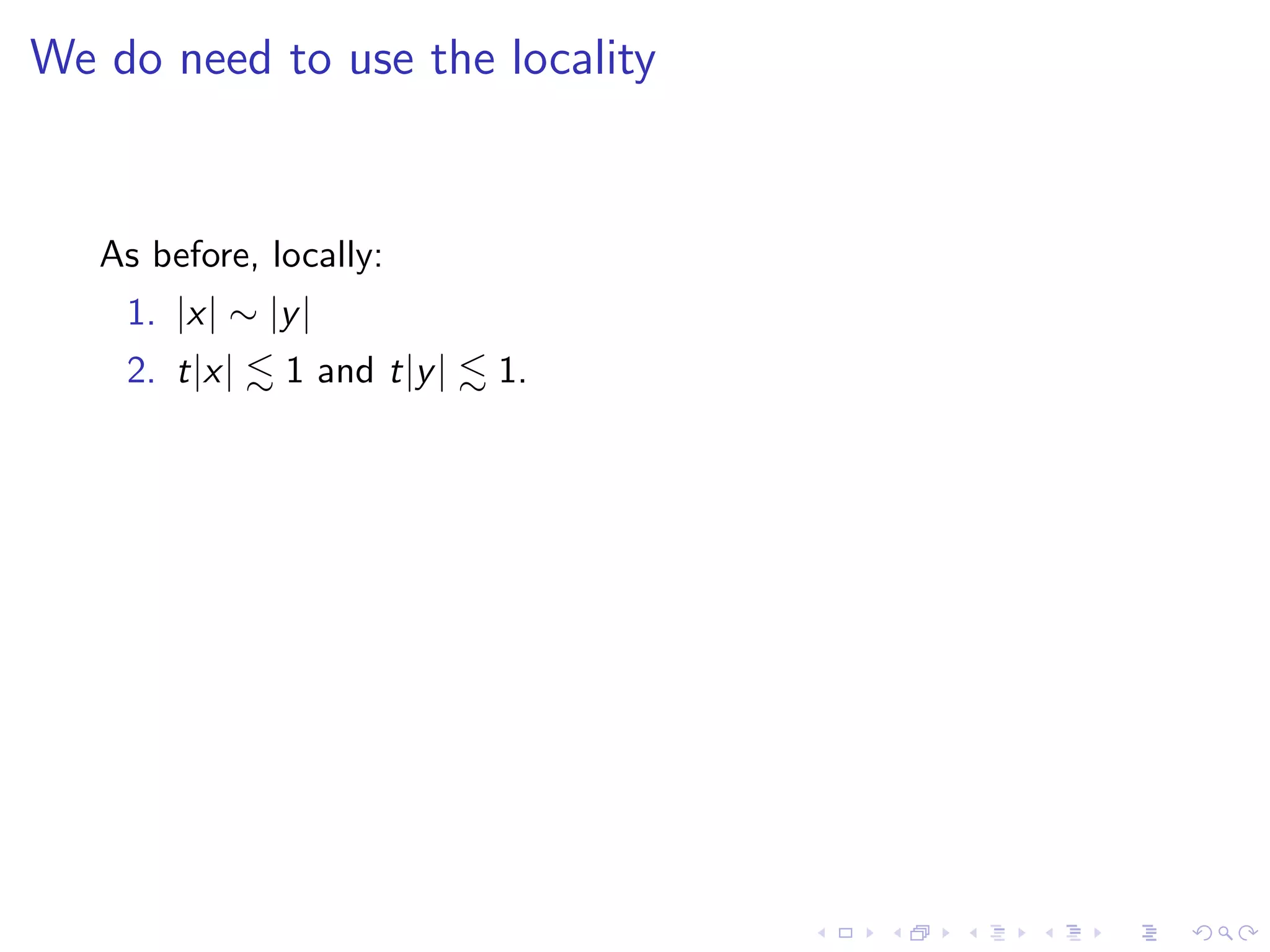
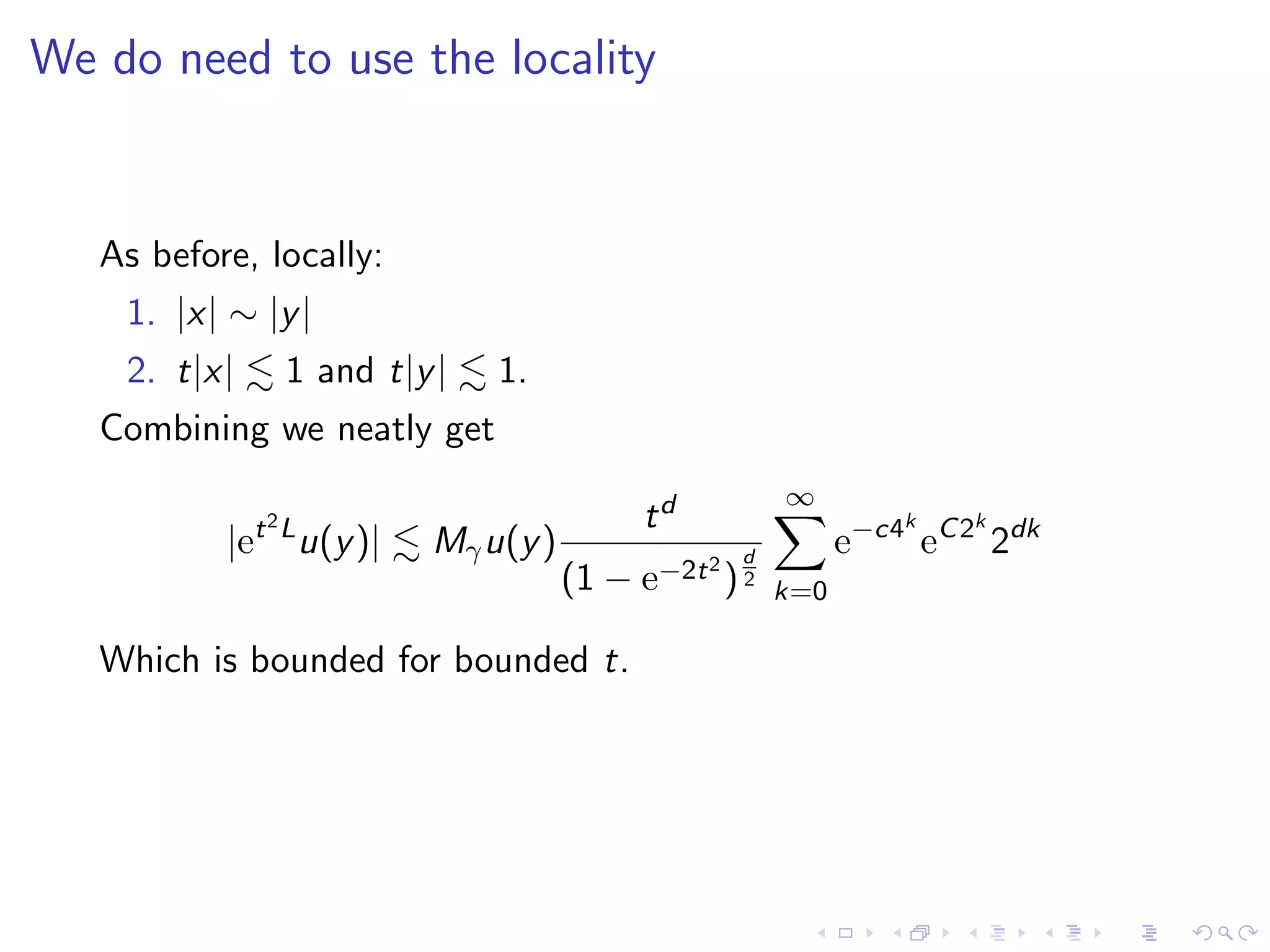
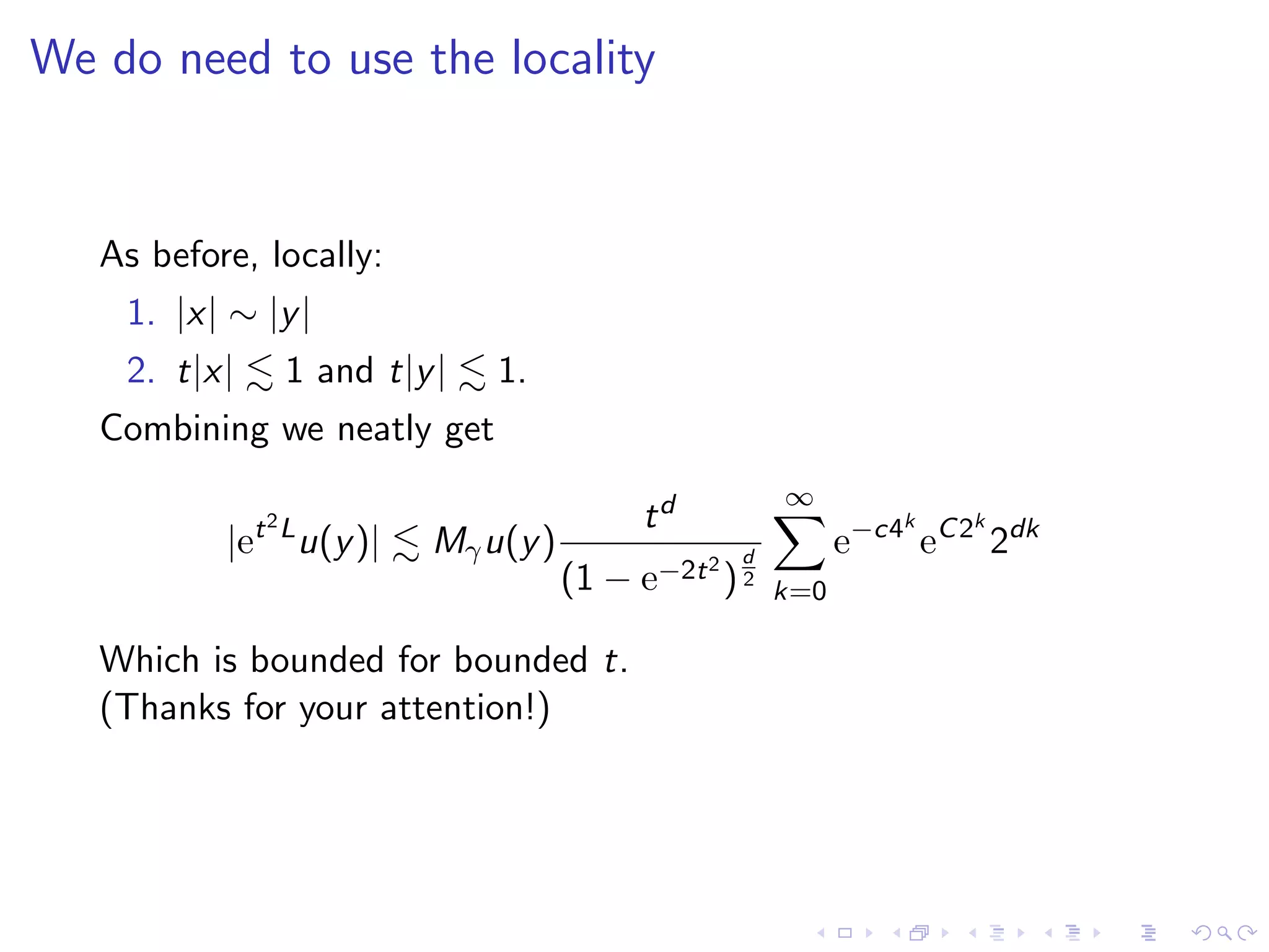
This document presents a summary of a talk on building a harmonic analytic theory for the Gaussian measure and the Ornstein-Uhlenbeck operator. It discusses how the Gaussian measure is non-doubling but satisfies a local doubling property. It introduces Gaussian cones and shows how they allow proving maximal function estimates for the Ornstein-Uhlenbeck semigroup in a similar way as for the heat semigroup. The talk outlines estimates for the Mehler kernel of the Ornstein-Uhlenbeck semigroup and combines them to obtain boundedness of the maximal function.

1. The Gaussian Hardy-Littlewood Maximal
Function
YFAW ’14 Lancaster, UK
Jonas Teuwen
Delft Institute for Applied Mathematics
Delft University of Technology, The Netherlands
24 April 2014

2. Introduction
Goal Build a satisfactory harmonic analytic theory for the
Gaussian measure
dγ(x) :=
e−|x|2
π
d
2
dx.
and the Ornstein-Uhlenbeck operator
L :=
1
2
∆ − x ·

3. Introduction
Goal Build a satisfactory harmonic analytic theory for the
Gaussian measure
dγ(x) :=
e−|x|2
π
d
2
dx.
and the Ornstein-Uhlenbeck operator
L :=
1
2
∆ − x ·
Just do it? Most theory relies on the doubling property of the
measure µ:
µ(B2r (x)) Cµ(Br (x))
uniformly in r and x.

4. As you might guess. . .
. . . the Gaussian measure is non-doubling
(but. . . maybe local?)
However, there is a kind of local doubling property! First this, we
define the admissible balls
Ba := {B(x, r) : r m(x)},
where,
m(x) := min 1,
1
|x|
.

5. As you might guess. . .
. . . the Gaussian measure is non-doubling
(but. . . maybe local?)
However, there is a kind of local doubling property! First this, we
define the admissible balls
Ba := {B(x, r) : r m(x)},
where,
m(x) := min 1,
1
|x|
.
For our admissible balls we then get the following lemma (Mauceri
& Meda):
Lemma
For all Br (x) ∈ Ba we have that
γ(B2r (x)) Cγ(Br (x)).

6. Some modifications – Gaussian cones
Gaussian harmonic analysis is local in the way that we use a cut-off
cone for our non-tangential maximal function
Γ
(A,a)
x (γ) := {(x, y) ∈ R2d
: |x − y| < At and t am(x)}.
−1
1
−1
1
1
x
y
t
Figure: This is a cut-off cone!

7. Gaussian cones – Useful consequences
1. On the cone Γ
(A,a)
x (γ) we have t|x| aA,
2. If |x − y| < At and t am(x) then |x| ∼ |y|.

8. Gaussian cones – Useful consequences
1. On the cone Γ
(A,a)
x (γ) we have t|x| aA,
2. If |x − y| < At and t am(x) then |x| ∼ |y|.
Using these two we have
1. If we have this then additionally t|y| 1
2. e−|x|2
∼ e−|y|2
.

9. Gaussian cones – Useful consequences
1. On the cone Γ
(A,a)
x (γ) we have t|x| aA,
2. If |x − y| < At and t am(x) then |x| ∼ |y|.
Using these two we have
1. If we have this then additionally t|y| 1
2. e−|x|2
∼ e−|y|2
.
Furthermore we define the annuli (Ck)k 0 through
Ck(x) :=
2Bt(x) if k = 0,
2k+1Bt(x) 2kBt(x) if k 1.

10. Only one theorem. . . – The Euclidean case
Theorem
Let u ∈ C∞
c (Rd ), then
sup
(y,t)∈Rd+1
+
|x−y|<t
|et2∆
u(y)| sup
r>0
1
|Br (x)| Br (x)
|u|dλ
Mu(x)
where λ is the Lebesgue measure.
The proof is straightforward, as et∆ is a convolution-type operator.
So et∆ = ρt ∗ u where
ρt(ξ) :=
e−|ξ|2/4t
(4πt)
d
2
.
is the heat kernel.
(There are many theorems about such convolution-type operators)

11. How to (ad hoc) prove it?
Let Ck := 2k+1B 2kB as before then
|et2∆
u(y)|
1
(4πt2)
d
2 Rd
e−|y−ξ|2/4t2
|u(ξ)| dξ
1
(4πt2)
d
2
∞
k=0
e−c4k
Ck (Bt (x))
|u(ξ)| dξ
1
(4πt2)
d
2
∞
k=0
e−c4k
|B2k+1t(x)|Mu(y)
Mu(y)
1
td
∞
k=0
e−c4k
td
2kd
.
Mu(y).
taking the supremum, and we are done.

12. Intermezzo: The Ornstein-Uhlenbeck semigroup
Remember the Ornstein-Uhlenbeck operator L?
L :=
1
2
∆ − x · .

13. Intermezzo: The Ornstein-Uhlenbeck semigroup
Remember the Ornstein-Uhlenbeck operator L?
L :=
1
2
∆ − x · .
L has the associated Ornstein-Uhlenbeck semigroup etL which in
its turn has an associated Schwartz kernel:
etL
u(x) =
Rd
Mt(x, ξ)u(ξ) dξ, u ∈ C∞
c (Rd
)
where the Mehler kernel Mt is given by
Mt(x, ξ) =
1
π
d
2
1
(1 − e−2t)
d
2
exp −
|e−tx − ξ|2
1 − e−2t
.
Not nearly as convenient to work with as the heat kernel!

14. Same ad hoc proof?
What goes wrong when we bluntly replace ∆ by L and the
Lebesgue measure by the Gaussian?

15. Same ad hoc proof?
What goes wrong when we bluntly replace ∆ by L and the
Lebesgue measure by the Gaussian?
On Ck we have a lower bound for |x − ξ|, so,
|e−t
x − ξ| |x − ξ| − (1 − e−t
)|x|
|x − ξ| − t|x|.
Here the cone condition t|x| 1 comes into play. Still, this is a bit
unsatisfactory. We require a Gaussian measure. So what can be
done?

16. Unsatisfactory? – Some observations
1. We use the Lebesgue measure again, while we want a
Gaussian theory. Perspective,. . .

17. Unsatisfactory? – Some observations
1. We use the Lebesgue measure again, while we want a
Gaussian theory. Perspective,. . .
2. In the end we want all admissibility paramaters and apertures
a and A. Proof gets very messy (e.g., Urbina and Pineda),

18. Unsatisfactory? – Some observations
1. We use the Lebesgue measure again, while we want a
Gaussian theory. Perspective,. . .
2. In the end we want all admissibility paramaters and apertures
a and A. Proof gets very messy (e.g., Urbina and Pineda),
3. Simple observations shows that the kernel should be
symmetric in its arguments against the Gaussian measure.

19. Unsatisfactory? – Some observations
1. We use the Lebesgue measure again, while we want a
Gaussian theory. Perspective,. . .
2. In the end we want all admissibility paramaters and apertures
a and A. Proof gets very messy (e.g., Urbina and Pineda),
3. Simple observations shows that the kernel should be
symmetric in its arguments against the Gaussian measure.
So, honouring these observations we come to. . .
etL
u(x) =
Rd
Mt(x, ξ)u(ξ) γ(dξ), u ∈ C∞
c (Rd
)
where the Mehler kernel Mt is given by
Mt(x, ξ) =
exp −e−2t |x − ξ|2
1 − e−2t
(1 − e−t)
d
2
exp −2e−t x, ξ
1 + e−t
(1 + e−t)
d
2
.

20. Estimating the Mehler kernel
On Ck this is now easier, for t 1 and t|x| 1:
Mt2 (x, ξ)
e−c4k
(1 − e−2t2
)
d
2
exp −2e−t2 x, ξ
1 + e−t2
e−c4k
(1 − e−2t2
)
d
2
exp(−| x, ξ |)
e−c4k
(1 − e−2t2
)
d
2
exp(| x, ξ − x |)e|x|2
e−c4k
(1 − e−2t2
)
d
2
exp(2k+1
t|x|)e|x|2

21. Was that enough? – Putting the things together
Let Ck := 2k+1B 2kB as before then
|et2L
u(y)|
1
(1 − e−2t2
)
d
2
∞
k=0
e−c4k
e2k+1t|y|
e|y|2
Ck (Bt (x))
|u| dγ
Mγu(y)
e|y|2
(1 − e−2t2
)
d
2
∞
k=0
e−c4k
e2k+1t|y|
γ(B2k+1t(x)).

22. Was that enough? – Putting the things together
Let Ck := 2k+1B 2kB as before then
|et2L
u(y)|
1
(1 − e−2t2
)
d
2
∞
k=0
e−c4k
e2k+1t|y|
e|y|2
Ck (Bt (x))
|u| dγ
Mγu(y)
e|y|2
(1 − e−2t2
)
d
2
∞
k=0
e−c4k
e2k+1t|y|
γ(B2k+1t(x)).
Estimating Gaussian balls:
γ(B2k+1t(x)) d 2d(k+1)
td
e2k+2t|x|
e−|x|2
.

23. We do need to use the locality
As before, locally:
1. |x| ∼ |y|
2. t|x| 1 and t|y| 1.

24. We do need to use the locality
As before, locally:
1. |x| ∼ |y|
2. t|x| 1 and t|y| 1.
Combining we neatly get
|et2L
u(y)| Mγu(y)
td
(1 − e−2t2
)
d
2
∞
k=0
e−c4k
eC2k
2dk
Which is bounded for bounded t.

25. We do need to use the locality
As before, locally:
1. |x| ∼ |y|
2. t|x| 1 and t|y| 1.
Combining we neatly get
|et2L
u(y)| Mγu(y)
td
(1 − e−2t2
)
d
2
∞
k=0
e−c4k
eC2k
2dk
Which is bounded for bounded t.
(Thanks for your attention!)