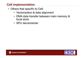
This document describes implementing 3D SPHARM surface registration on a Cell processor. It discusses SPHARM expansion and registration, calculating rotation coefficients, root mean square distance, and implementations in Matlab and on the Cell processor. The Cell implementation uses loop fusion, lookup tables, and optimizations for the Cell architecture like vectorization and data alignment. Performance analysis shows a dramatic increase in speed on the Cell due to its architecture and algorithm optimizations. Care is needed for data placement and transfer due to limited local store.

1. Implementing 3D SPHARM Surfaces
Registration on Cell Processor
Huian Li (huili@indiana.edu) Mi Yan (miyan@us.ibm.com)
Robert Henschel (rhensche@indiana edu)
(rhensche@indiana.edu) Li Shen (shenli@iupui edu)
(shenli@iupui.edu)
July 29, 2009

2. Contents
• SPHARM registration
• Matlab implementation
• Cell implementation
• Performance Analysis
• Conclusion

3. SPHARM Surfaces
• R di l and stellar surfaces
Radial d t ll f
• Simply connected, arbitrarily shaped
• Vision, graphics, imaging, bioinformatics

4. SPHARM Expansion
( )  (x y z)
(,)  (x,y,z)
( )
(,) (x,y,z)
( )
Area-preserving
mapping

5. SHREC
(a) template, (b) object, (c) after ICP, (d) after
registration of p
g parameterization

6. Calculation of coefficients
• After rotating the parameter net on the surface in
Euler angles (α, β, γ), new coefficients will be:
l
c (  ) 
m
l 
nl
D l
mn (  ) c l
n
where
min( l  n ,l  m )
D mn ( )  e (  i m  in ) (
l
 (  1) t d mnt (  ))
t  max( 0 , n  m )
l
and
(l  n)!(l  n)!(l  m)!(l  m)!  
d mnt (  ) 
l
 (cos ) ( 2l nm2t ) (sin ) ( 2t mn )
(l  n  t )!(l  m  t )!(t  m  n)!t! 2 2

7. RMSD
• RMSD (Root Mean Square Distance): distance
between two SPHARM models
L max l
1
RMSD 
4
 
l0 m l
|| c 1ml  c 2 , l || 2
,
m
m m
c and c
1 ,l 2 ,l are coefficients of two
SPHARM models

8. Matlab implementation
• A straightforward implementation in Matlab:
for l = 0 Lmax
0,
for m = -l, l
for n = -l, l
l
for t = max(0, n-m), min(l+m, l-n)
... performing calculations ...
• One rotation for Lmax = 50 took 823 seconds on 2GHz quad
quad-
core Intel Xeon E5335

9. Cell B.E.

10. Cell implementation
• Domain decomposition:
for l = 0, Lmax
for m = -l l
l,
for n = -l, l
for t = max(0 n-m) min(l+m l-n)
max(0, n m), min(l+m, l n)
... calculations ...
• Decomposition along l leads to work load
imbalance among SPUs
• Decomposition along m creates unnecessary data
p g y
communication

11. Cell implementation
• Loop fusion:
for l = 0, Lmax
for m = -l l
l,
for n = -l, l
for t = max(0 n-m) min(l+m l-n)
max(0, n m), min(l+m, l n)
... calculations ...
• Unique index for combined loop:
f(l, m) = l2 + m + l
• W kl d f each SPE :
Workload for h
(Lmax + 1)2/(total # of SPEs)

12. Cell implementation
• Lookup table T for factorial
• Transform exponentials & multiplications into
multiplications & additions respectively
additions, respectively.
(l  n)!(l  n)!(l  m)!(l  m)!  
d l
( )   (cos ) ( 2l nm2t ) (sin ) ( 2t mn )
(l  n  t )!(l  m  t )!(t  m  n)!t!
mnt
2 2
 exp(
1
 (T (l  n )  T (l  n )  T (l  m )  T (l  m ))
2
 T (l  n  t )  T (l  m  t )  T (t  m  n )  T (t )
 
 ( 2l  n  m  2t )  log(cos )  ( 2t  m  n )  log(sin ))
2 2

13. Cell implementation
• Others that specific to Cell:
• Vectorization & data alignment
• DMA data transfer between main memory &
local store
• SPU d decrementert

14. Cell implementation
• Single p
g precision vs. double p
precision: all data in single p
g precision

15. Cell implementation
• Single p
g precision vs. double p
precision: p
partial data in double p
precision

16. Cell implementation
• Single p
g precision vs. double p
precision: all critical data in double p
precision

17. Performance analysis
Performance of one rotation on Cell BE
1.8
18
1.6
1.4
s)
Time (seconds
1.2
1
0.8
0.6
0.4
04
T
0.2
0
1 2 4 8 16
Number of SPEs

18. Performance analysis
Performance of finding the shortest
distance at Level 3 on Cell BE
7000
6000
5000
s)
seconds
4000
Time (s
3000 GNU gcc
IBM xlc
2000
1000
0
4 8 12 16
Number of SPEs

19. Conclusion
• Performance increases dramatically on Cell due to
its unique architecture and algorithm optimization.
• Carefulness must be taken for data placement due
to limited local store.
• Carefulness must also be taken for data transfer
between local store and main memory.

20. The End
Questions?