Deep Learning forComputer Vision
Feature Detectors: SIFT and Variants
Vineeth N Balasubramanian
Department of Computer Science and Engineering
Indian Institute of Technology, Hyderabad
Vineeth N B (IIT-H) §2.4 Feature Detectors 1 / 28
2.
SIFT: Scale InvariantFeature Transform
David G. Lowe, Distinctive Image Features from Scale-invariant Keypoints, IJCV 2004
Over 50000 citations
Transforms image data into scale-invariant coordinates
Fundamental to many core vision problems/applications:
Recognition, Motion tracking, Multiview geometry
Vineeth N B (IIT-H) §2.4 Feature Detectors 2 / 28
3.
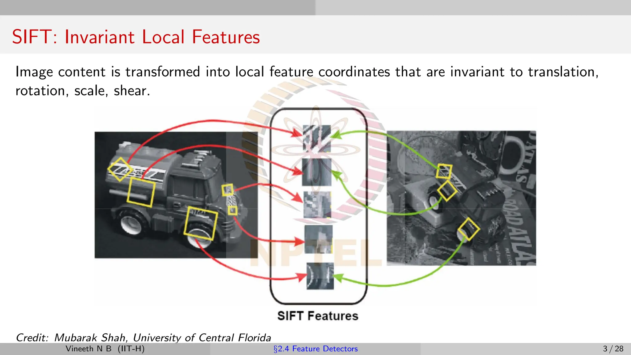
SIFT: Invariant LocalFeatures
Image content is transformed into local feature coordinates that are invariant to translation,
rotation, scale, shear.
Credit: Mubarak Shah, University of Central Florida
Vineeth N B (IIT-H) §2.4 Feature Detectors 3 / 28
4.
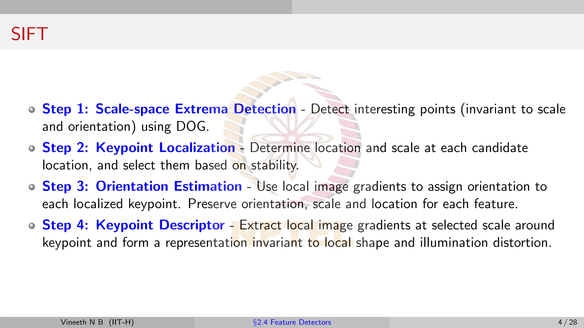
SIFT
Step 1: Scale-spaceExtrema Detection - Detect interesting points (invariant to scale
and orientation) using DOG.
Step 2: Keypoint Localization - Determine location and scale at each candidate
location, and select them based on stability.
Step 3: Orientation Estimation - Use local image gradients to assign orientation to
each localized keypoint. Preserve orientation, scale and location for each feature.
Step 4: Keypoint Descriptor - Extract local image gradients at selected scale around
keypoint and form a representation invariant to local shape and illumination distortion.
Vineeth N B (IIT-H) §2.4 Feature Detectors 4 / 28
5.
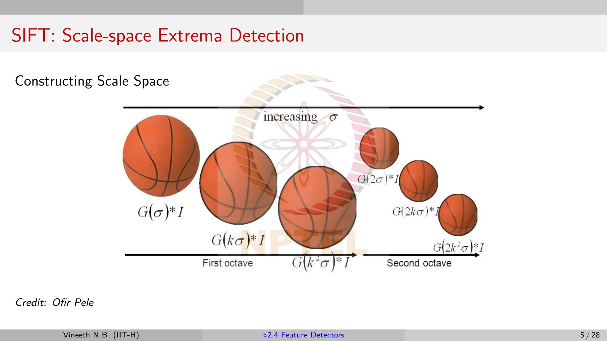
SIFT: Scale-space ExtremaDetection
Constructing Scale Space
Credit: Ofir Pele
Vineeth N B (IIT-H) §2.4 Feature Detectors 5 / 28
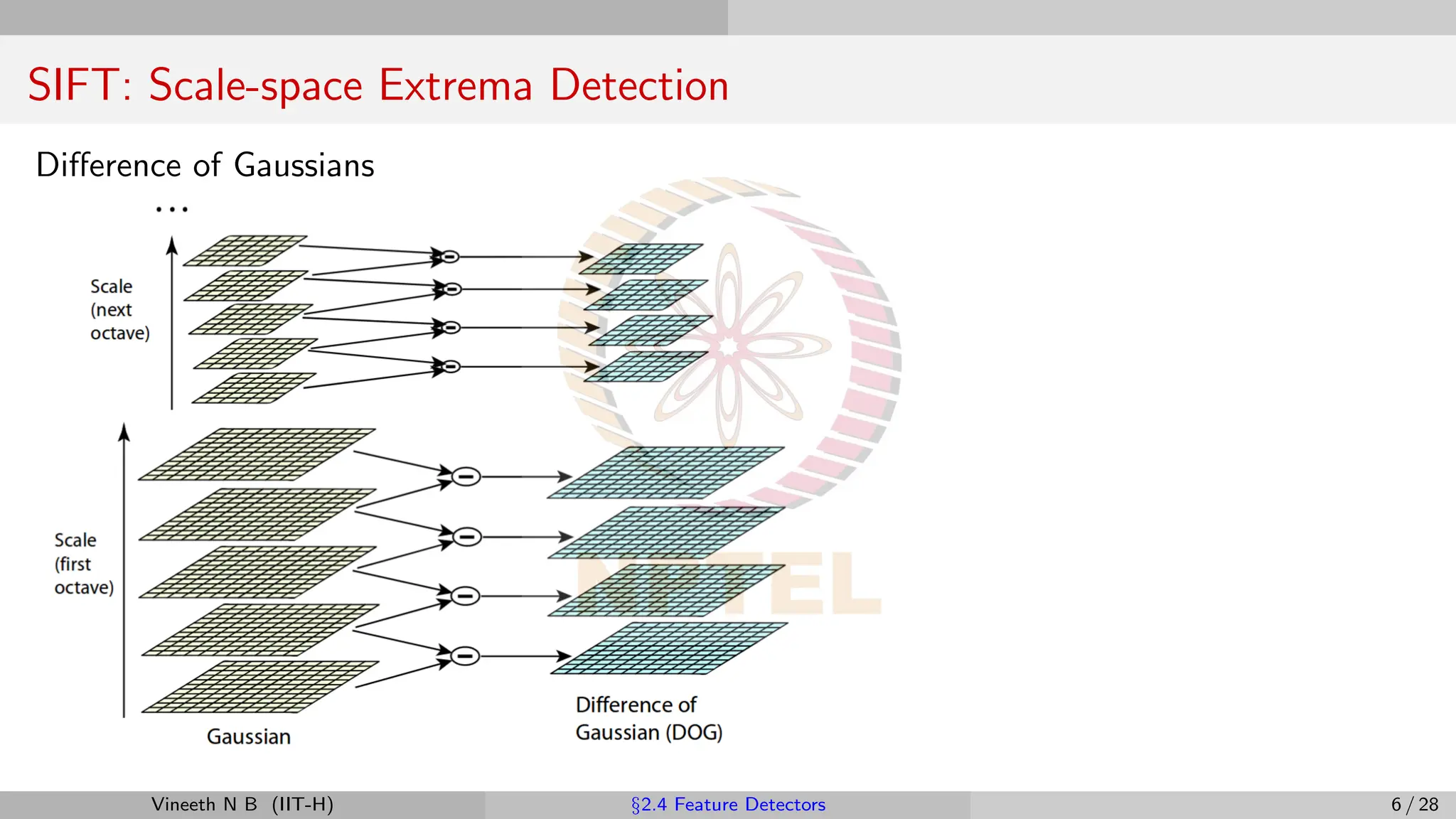
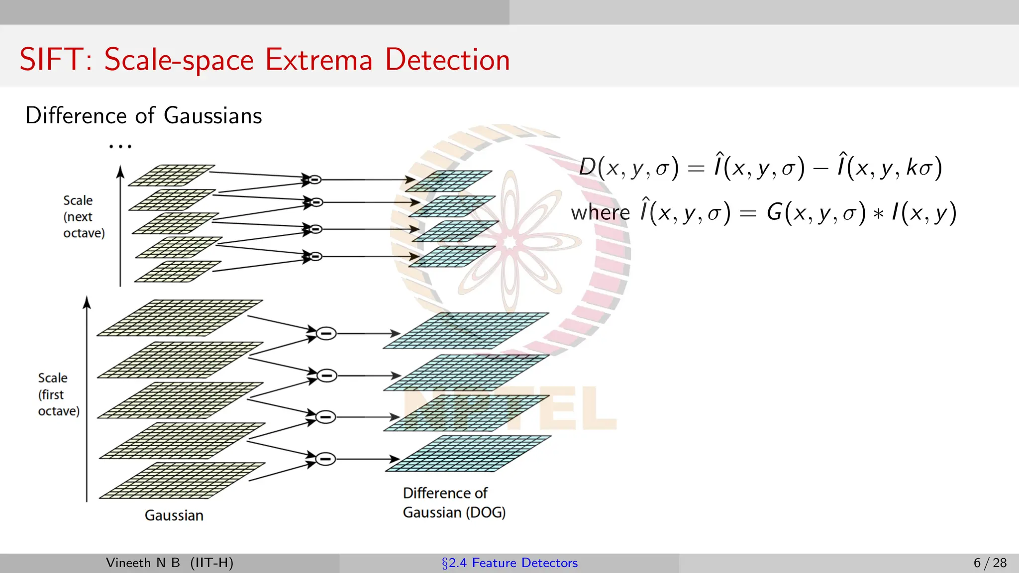
6.
SIFT: Scale-space ExtremaDetection
Difference of Gaussians
Vineeth N B (IIT-H) §2.4 Feature Detectors 6 / 28
7.
SIFT: Scale-space ExtremaDetection
Difference of Gaussians
D(x, y, σ) = ˆ
I(x, y, σ) − ˆ
I(x, y, kσ)
where ˆ
I(x, y, σ) = G(x, y, σ) ∗ I(x, y)
Vineeth N B (IIT-H) §2.4 Feature Detectors 6 / 28
8.
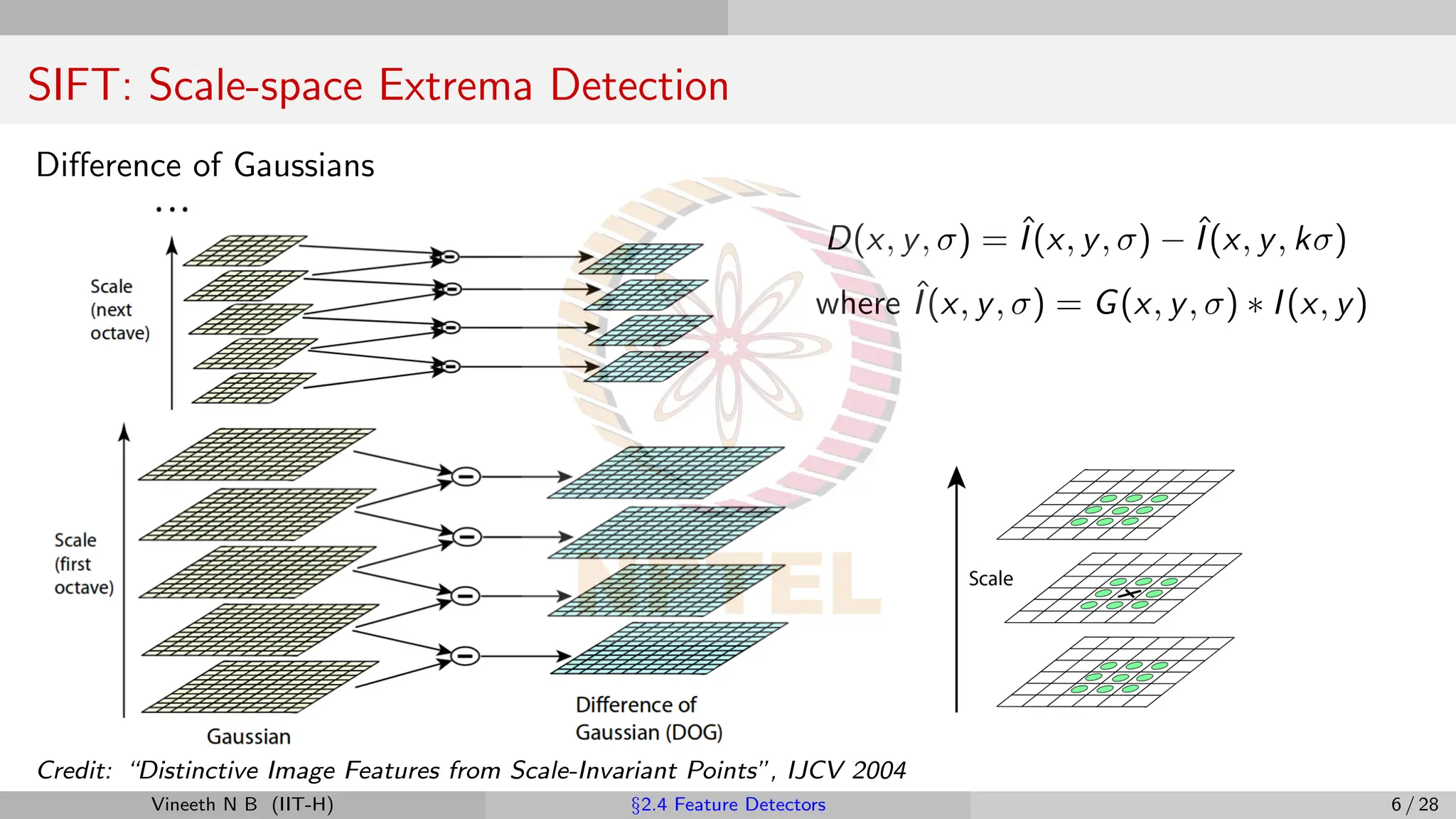
SIFT: Scale-space ExtremaDetection
Difference of Gaussians
D(x, y, σ) = ˆ
I(x, y, σ) − ˆ
I(x, y, kσ)
where ˆ
I(x, y, σ) = G(x, y, σ) ∗ I(x, y)
Credit: “Distinctive Image Features from Scale-Invariant Points”, IJCV 2004
Vineeth N B (IIT-H) §2.4 Feature Detectors 6 / 28
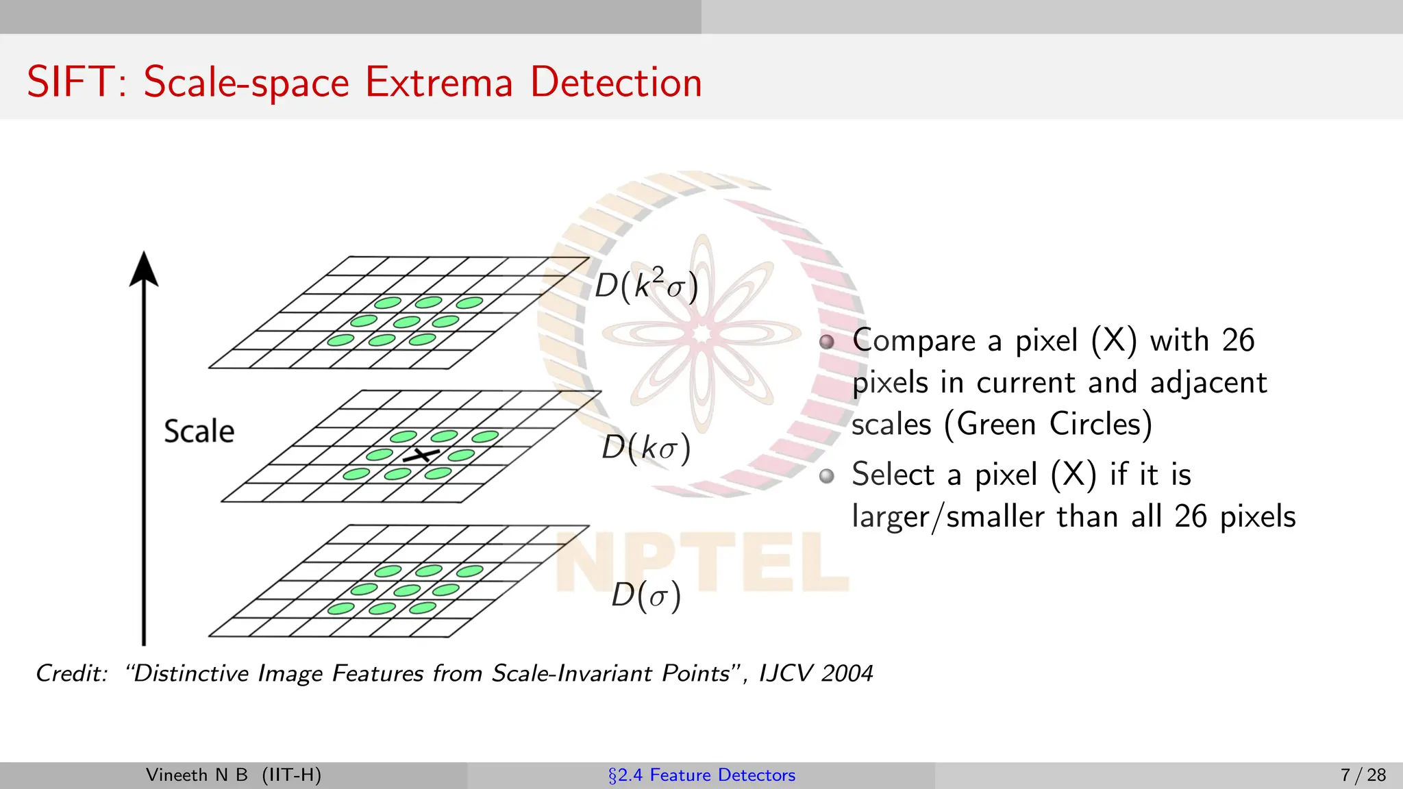
9.
SIFT: Scale-space ExtremaDetection
D(k2
σ)
D(kσ)
D(σ)
Compare a pixel (X) with 26
pixels in current and adjacent
scales (Green Circles)
Select a pixel (X) if it is
larger/smaller than all 26 pixels
Credit: “Distinctive Image Features from Scale-Invariant Points”, IJCV 2004
Vineeth N B (IIT-H) §2.4 Feature Detectors 7 / 28
10.
SIFT: Scale-space ExtremaDetection
D(k2
σ)
D(kσ)
D(σ)
Compare a pixel (X) with 26
pixels in current and adjacent
scales (Green Circles)
Select a pixel (X) if it is
larger/smaller than all 26 pixels
Credit: “Distinctive Image Features from Scale-Invariant Points”, IJCV 2004
Vineeth N B (IIT-H) §2.4 Feature Detectors 7 / 28
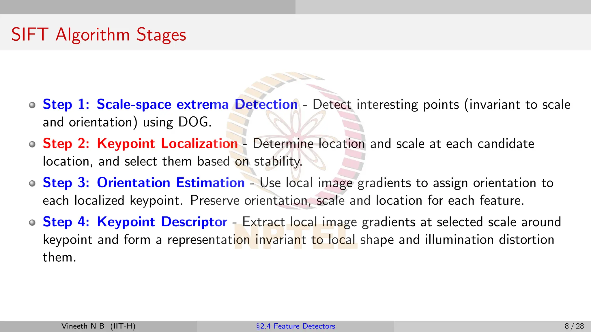
11.
SIFT Algorithm Stages
Step1: Scale-space extrema Detection - Detect interesting points (invariant to scale
and orientation) using DOG.
Step 2: Keypoint Localization - Determine location and scale at each candidate
location, and select them based on stability.
Step 3: Orientation Estimation - Use local image gradients to assign orientation to
each localized keypoint. Preserve orientation, scale and location for each feature.
Step 4: Keypoint Descriptor - Extract local image gradients at selected scale around
keypoint and form a representation invariant to local shape and illumination distortion
them.
Vineeth N B (IIT-H) §2.4 Feature Detectors 8 / 28
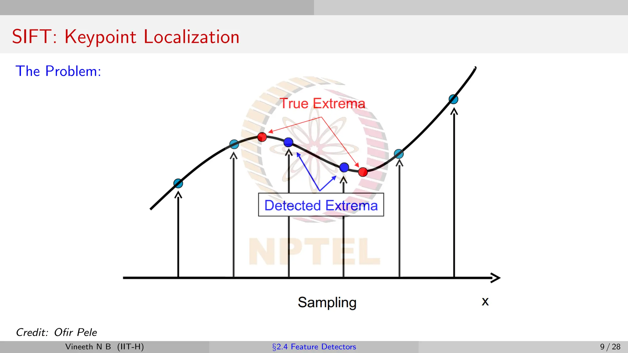
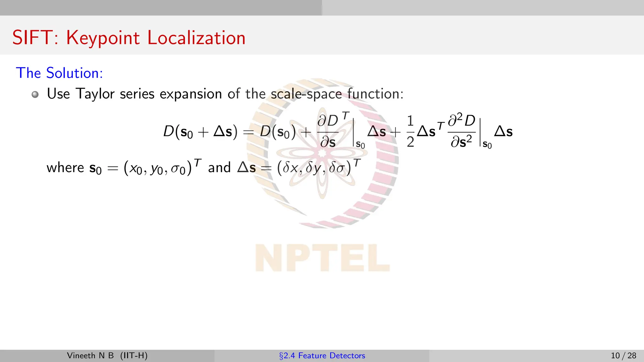
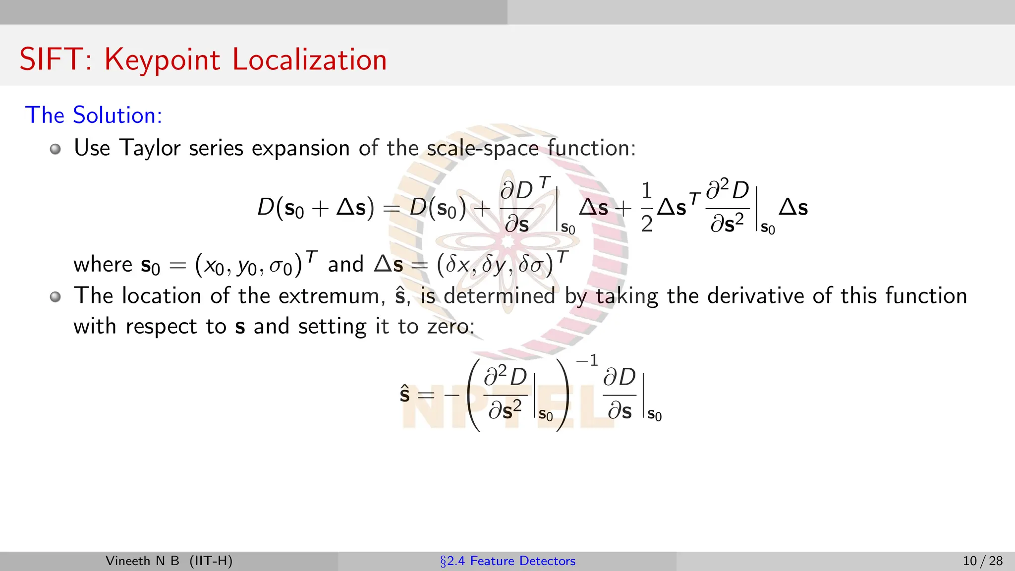
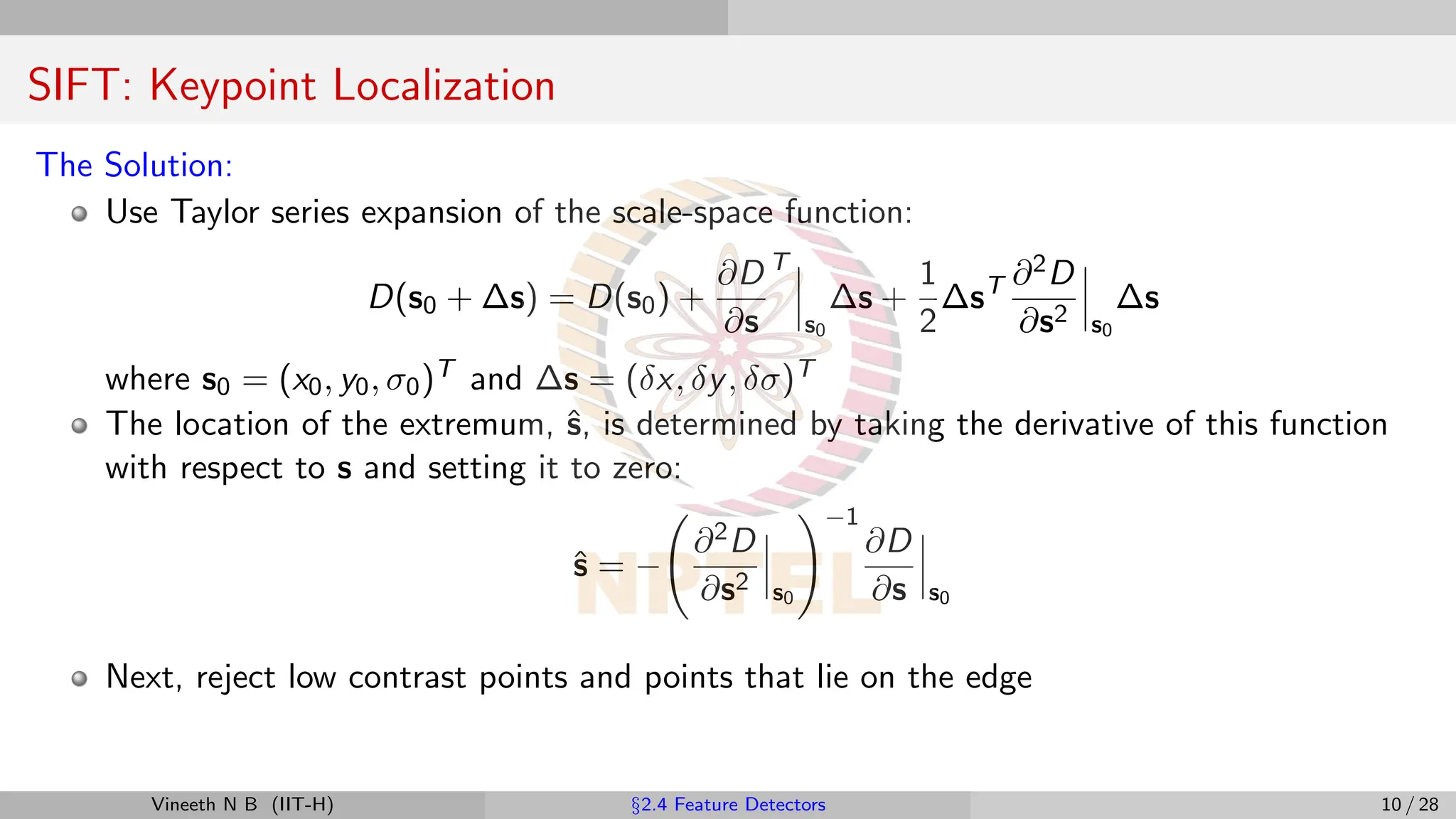
SIFT: Keypoint Localization
TheSolution:
Use Taylor series expansion of the scale-space function:
D(s0 + ∆s) = D(s0) +
∂D
∂s
T
s0
∆s +
1
2
∆sT ∂2D
∂s2 s0
∆s
where s0 = (x0, y0, σ0)T and ∆s = (δx, δy, δσ)T
Vineeth N B (IIT-H) §2.4 Feature Detectors 10 / 28
14.
SIFT: Keypoint Localization
TheSolution:
Use Taylor series expansion of the scale-space function:
D(s0 + ∆s) = D(s0) +
∂D
∂s
T
s0
∆s +
1
2
∆sT ∂2D
∂s2 s0
∆s
where s0 = (x0, y0, σ0)T and ∆s = (δx, δy, δσ)T
The location of the extremum, ŝ, is determined by taking the derivative of this function
with respect to s and setting it to zero:
ŝ = −
∂2D
∂s2 s0
!−1
∂D
∂s s0
Vineeth N B (IIT-H) §2.4 Feature Detectors 10 / 28
15.
SIFT: Keypoint Localization
TheSolution:
Use Taylor series expansion of the scale-space function:
D(s0 + ∆s) = D(s0) +
∂D
∂s
T
s0
∆s +
1
2
∆sT ∂2D
∂s2 s0
∆s
where s0 = (x0, y0, σ0)T and ∆s = (δx, δy, δσ)T
The location of the extremum, ŝ, is determined by taking the derivative of this function
with respect to s and setting it to zero:
ŝ = −
∂2D
∂s2 s0
!−1
∂D
∂s s0
Next, reject low contrast points and points that lie on the edge
Vineeth N B (IIT-H) §2.4 Feature Detectors 10 / 28
16.
SIFT: Keypoint Localization
TheSolution:
Use Taylor series expansion of the scale-space function:
D(s0 + ∆s) = D(s0) +
∂D
∂s
T
s0
∆s +
1
2
∆sT ∂2D
∂s2 s0
∆s
where s0 = (x0, y0, σ0)T and ∆s = (δx, δy, δσ)T
The location of the extremum, ŝ, is determined by taking the derivative of this function
with respect to s and setting it to zero:
ŝ = −
∂2D
∂s2 s0
!−1
∂D
∂s s0
Next, reject low contrast points and points that lie on the edge
Low contrast points elimination:
Reject keypoint if D(ŝ) is smaller than 0.03 (assuming image values are normalized in [0,1])
Vineeth N B (IIT-H) §2.4 Feature Detectors 10 / 28
17.
SIFT: Keypoint Localization
Rejectpoints with strong edge response
in one direction only
Edge Elimination - How?
Vineeth N B (IIT-H) §2.4 Feature Detectors 11 / 28
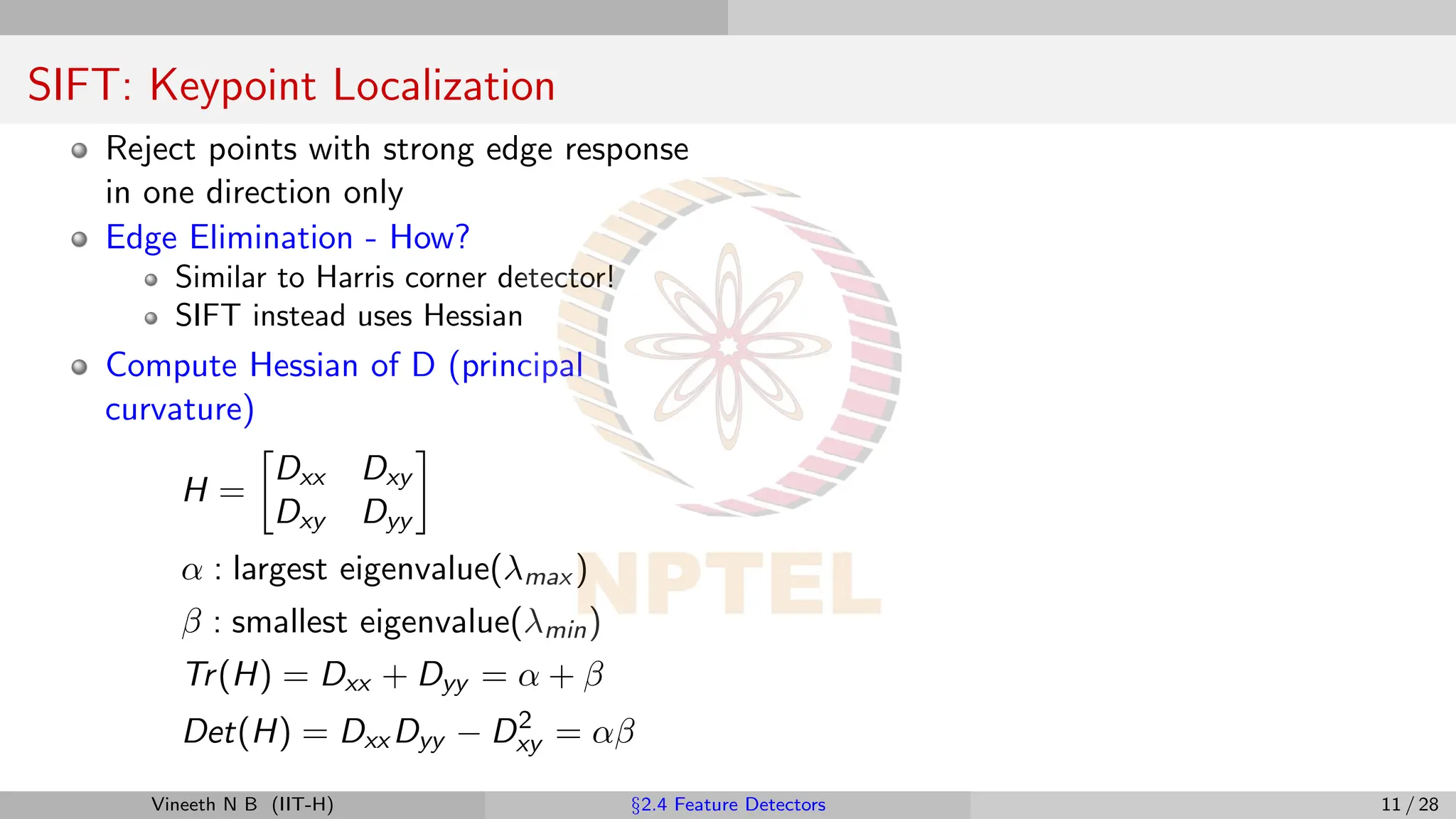
18.
SIFT: Keypoint Localization
Rejectpoints with strong edge response
in one direction only
Edge Elimination - How?
Similar to Harris corner detector!
SIFT instead uses Hessian
Compute Hessian of D (principal
curvature)
H =
Dxx Dxy
Dxy Dyy
α : largest eigenvalue(λmax )
β : smallest eigenvalue(λmin)
Tr(H) = Dxx + Dyy = α + β
Det(H) = Dxx Dyy − D2
xy = αβ
Vineeth N B (IIT-H) §2.4 Feature Detectors 11 / 28
19.
SIFT: Keypoint Localization
Rejectpoints with strong edge response
in one direction only
Edge Elimination - How?
Similar to Harris corner detector!
SIFT instead uses Hessian
Compute Hessian of D (principal
curvature)
H =
Dxx Dxy
Dxy Dyy
α : largest eigenvalue(λmax )
β : smallest eigenvalue(λmin)
Tr(H) = Dxx + Dyy = α + β
Det(H) = Dxx Dyy − D2
xy = αβ
Evaluate ratio
Tr(H)2
Det(H)
=
(α + β)2
αβ
=
(rβ + β)2
rβ2
Tr(H)2
Det(H)
=
(r + 1)2
r
where r =
α
β
Vineeth N B (IIT-H) §2.4 Feature Detectors 11 / 28
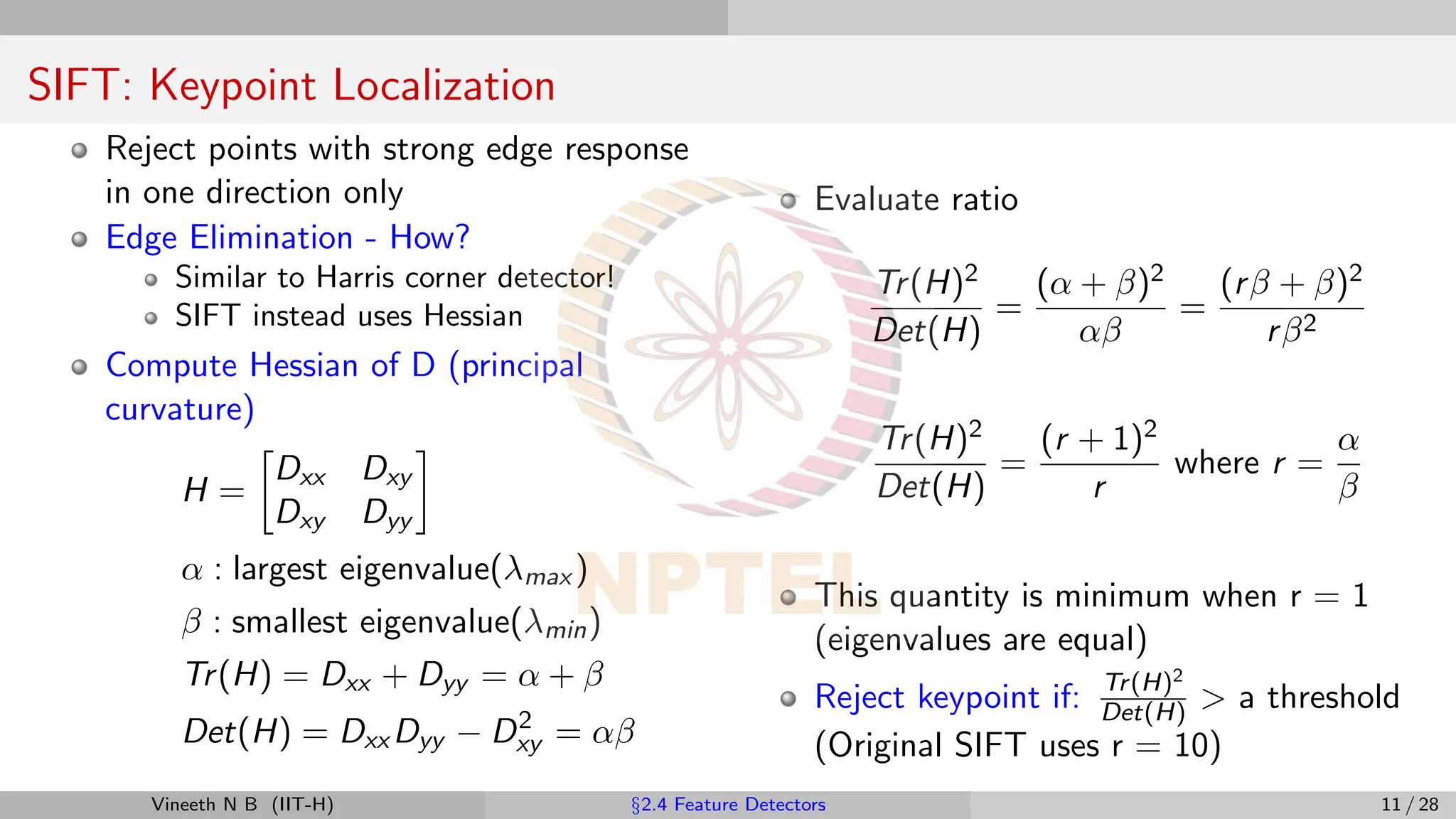
20.
SIFT: Keypoint Localization
Rejectpoints with strong edge response
in one direction only
Edge Elimination - How?
Similar to Harris corner detector!
SIFT instead uses Hessian
Compute Hessian of D (principal
curvature)
H =
Dxx Dxy
Dxy Dyy
α : largest eigenvalue(λmax )
β : smallest eigenvalue(λmin)
Tr(H) = Dxx + Dyy = α + β
Det(H) = Dxx Dyy − D2
xy = αβ
Evaluate ratio
Tr(H)2
Det(H)
=
(α + β)2
αβ
=
(rβ + β)2
rβ2
Tr(H)2
Det(H)
=
(r + 1)2
r
where r =
α
β
This quantity is minimum when r = 1
(eigenvalues are equal)
Reject keypoint if: Tr(H)2
Det(H) a threshold
(Original SIFT uses r = 10)
Vineeth N B (IIT-H) §2.4 Feature Detectors 11 / 28
21.
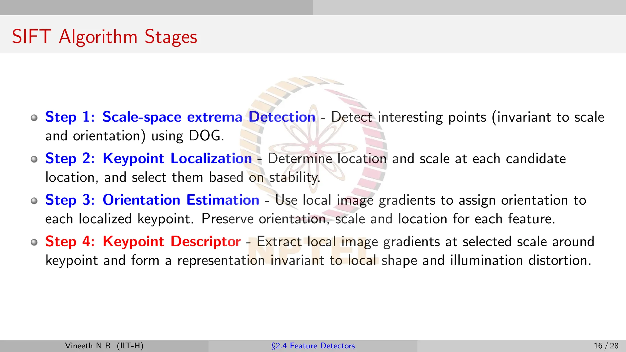
SIFT Algorithm Stages
Step1: Scale-space extrema Detection - Detect interesting points (invariant to scale
and orientation) using DOG.
Step 2: Keypoint Localization - Determine location and scale at each candidate
location, and select them based on stability.
Step 3: Orientation Estimation - Use local image gradients to assign orientation to
each localized keypoint. Preserve orientation, scale and location for each feature.
Step 4: Keypoint Descriptor - Extract local image gradients at selected scale around
keypoint and form a representation invariant to local shape and illumination distortion
them.
Vineeth N B (IIT-H) §2.4 Feature Detectors 12 / 28
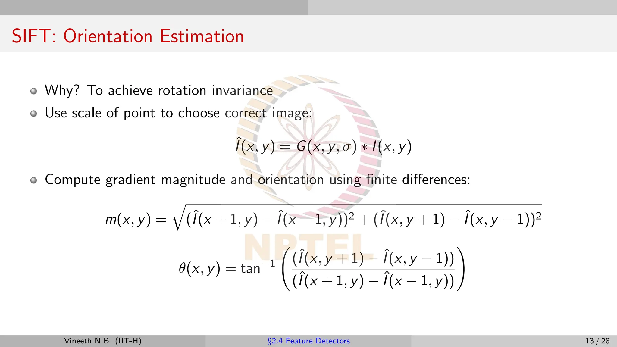
SIFT: Orientation Estimation
Why?To achieve rotation invariance
Use scale of point to choose correct image:
ˆ
I(x, y) = G(x, y, σ) ∗ I(x, y)
Compute gradient magnitude and orientation using finite differences:
m(x, y) =
q
(ˆ
I(x + 1, y) − ˆ
I(x − 1, y))2 + (ˆ
I(x, y + 1) − ˆ
I(x, y − 1))2
θ(x, y) = tan−1 (ˆ
I(x, y + 1) − ˆ
I(x, y − 1))
(ˆ
I(x + 1, y) − ˆ
I(x − 1, y))
!
Vineeth N B (IIT-H) §2.4 Feature Detectors 13 / 28
25.
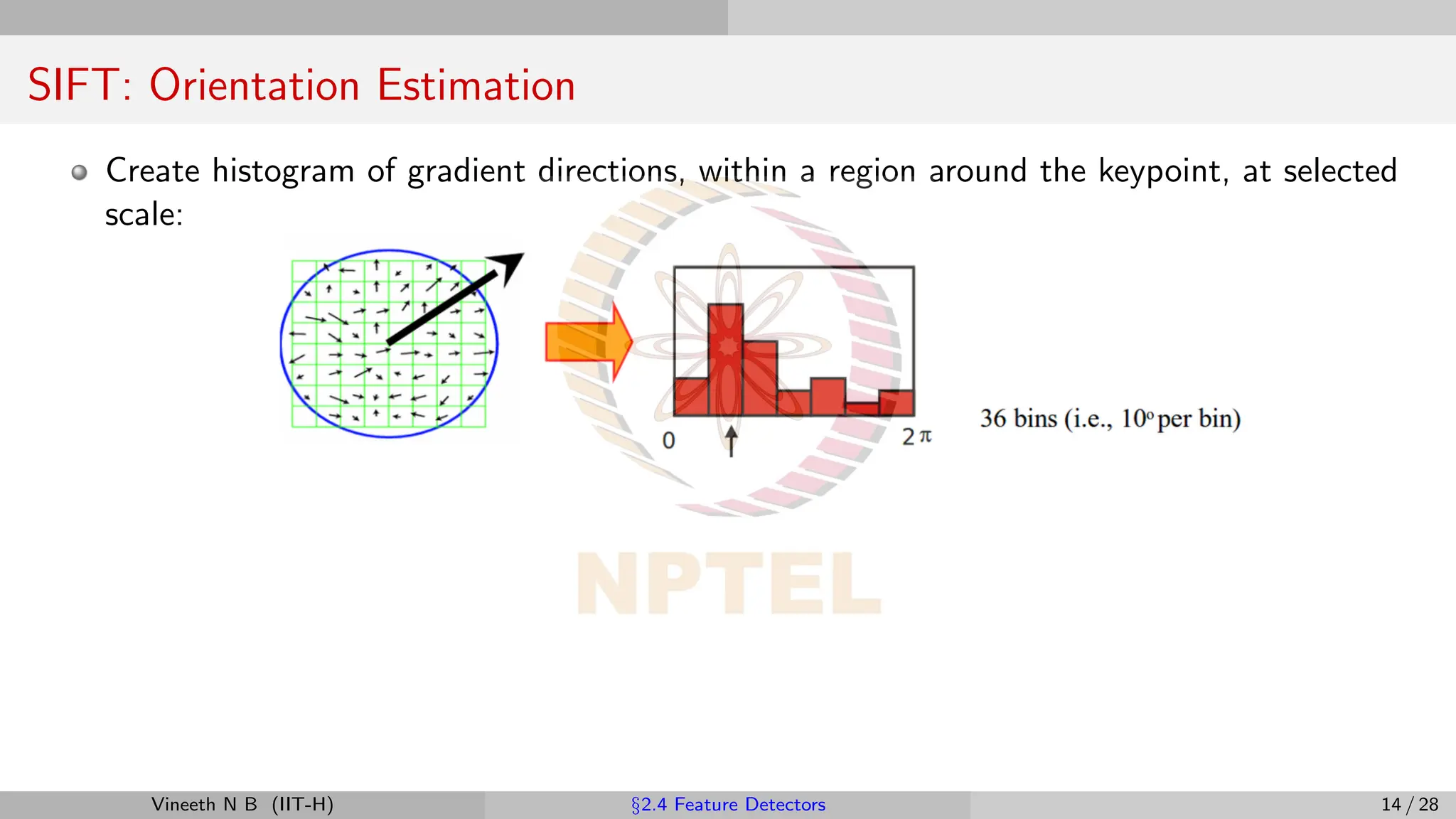
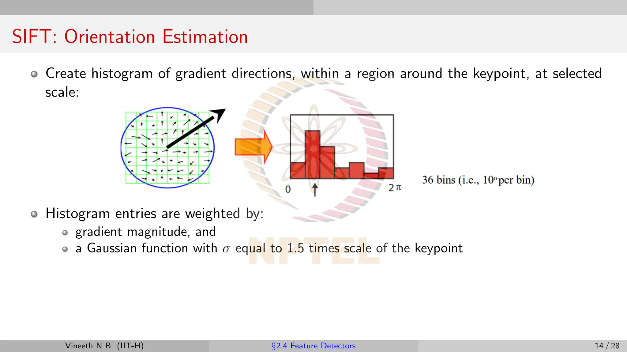
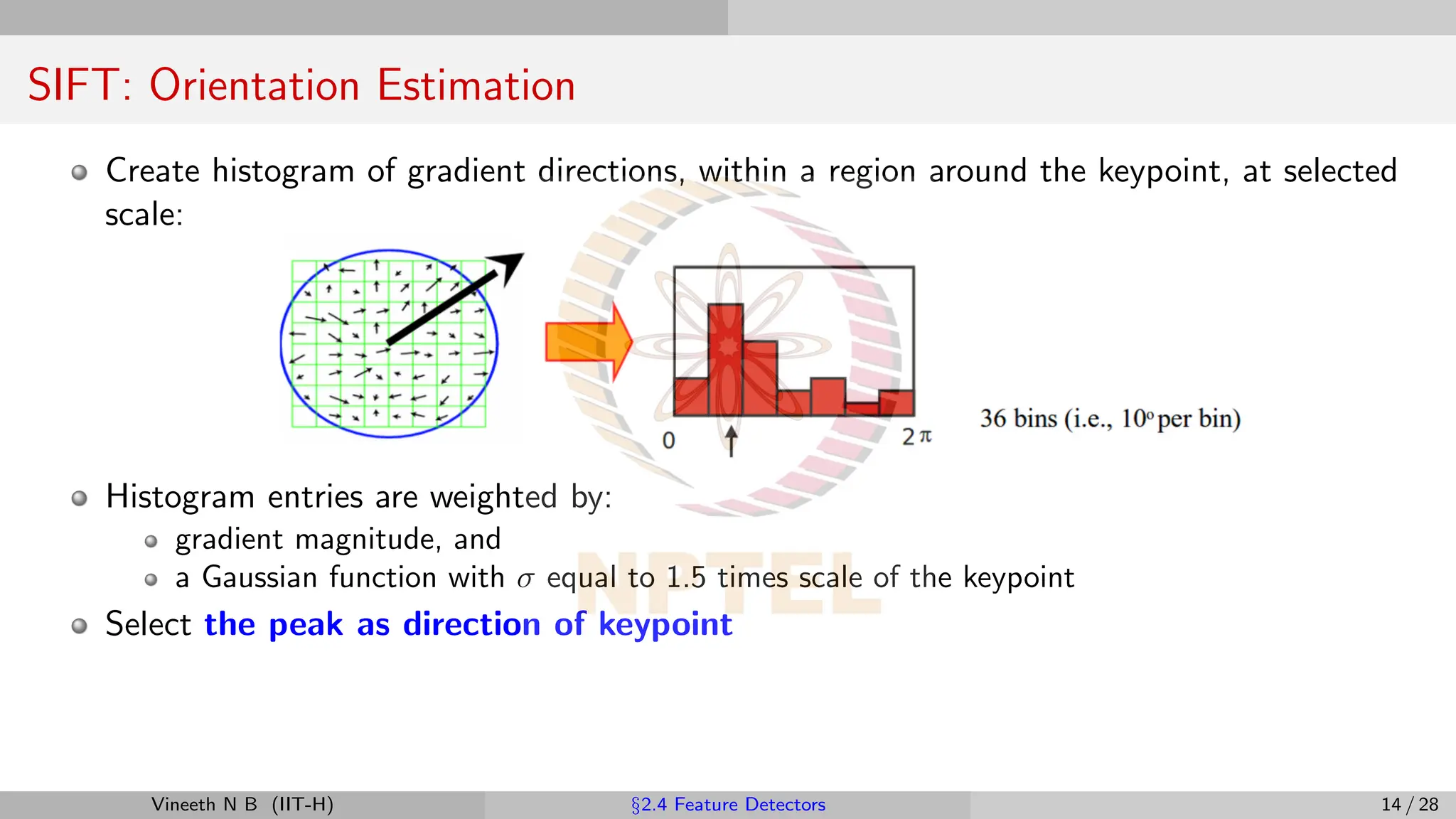
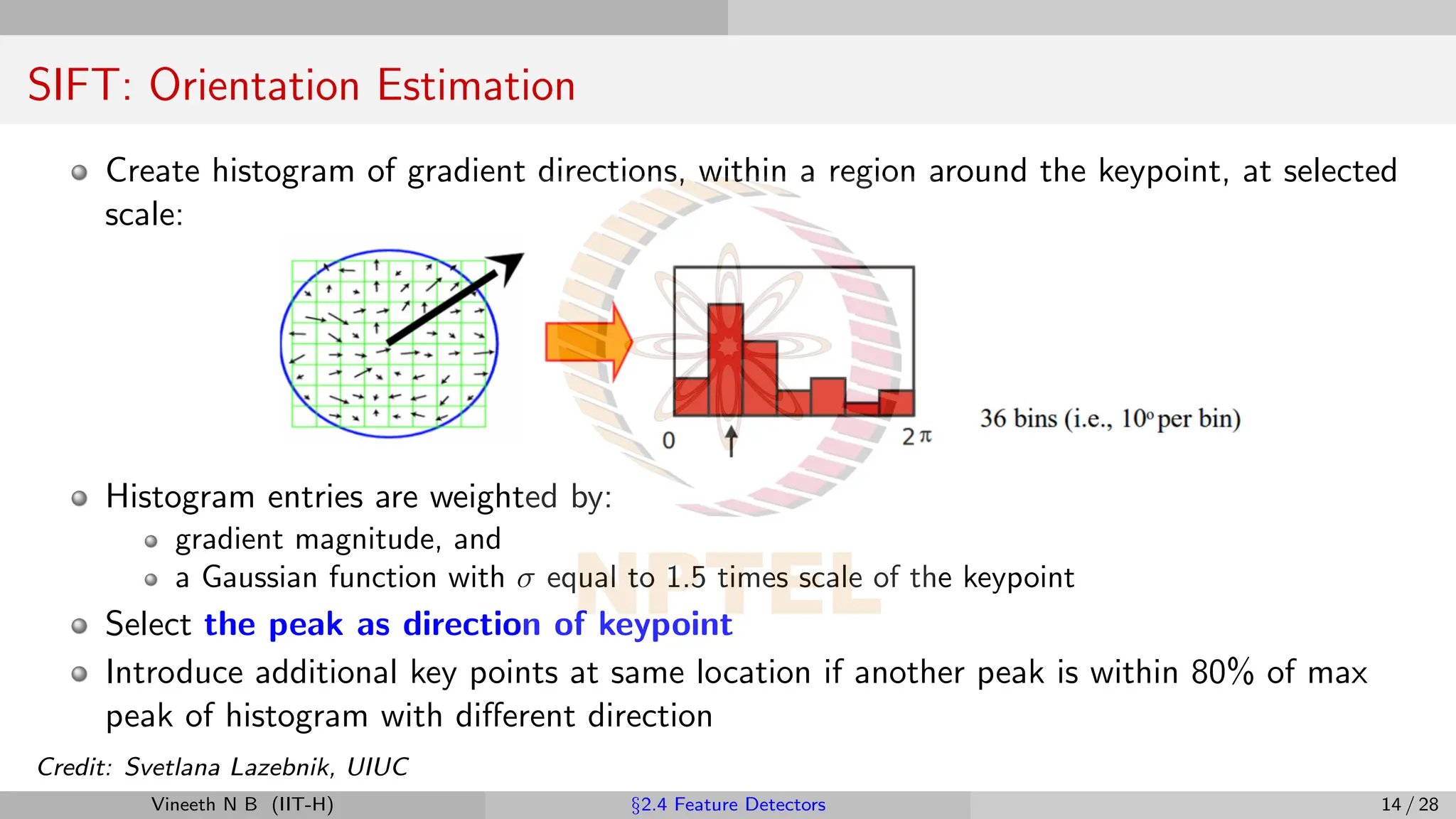
SIFT: Orientation Estimation
Createhistogram of gradient directions, within a region around the keypoint, at selected
scale:
Vineeth N B (IIT-H) §2.4 Feature Detectors 14 / 28
26.
SIFT: Orientation Estimation
Createhistogram of gradient directions, within a region around the keypoint, at selected
scale:
Histogram entries are weighted by:
gradient magnitude, and
a Gaussian function with σ equal to 1.5 times scale of the keypoint
Vineeth N B (IIT-H) §2.4 Feature Detectors 14 / 28
27.
SIFT: Orientation Estimation
Createhistogram of gradient directions, within a region around the keypoint, at selected
scale:
Histogram entries are weighted by:
gradient magnitude, and
a Gaussian function with σ equal to 1.5 times scale of the keypoint
Select the peak as direction of keypoint
Vineeth N B (IIT-H) §2.4 Feature Detectors 14 / 28
28.
SIFT: Orientation Estimation
Createhistogram of gradient directions, within a region around the keypoint, at selected
scale:
Histogram entries are weighted by:
gradient magnitude, and
a Gaussian function with σ equal to 1.5 times scale of the keypoint
Select the peak as direction of keypoint
Introduce additional key points at same location if another peak is within 80% of max
peak of histogram with different direction
Credit: Svetlana Lazebnik, UIUC
Vineeth N B (IIT-H) §2.4 Feature Detectors 14 / 28
29.
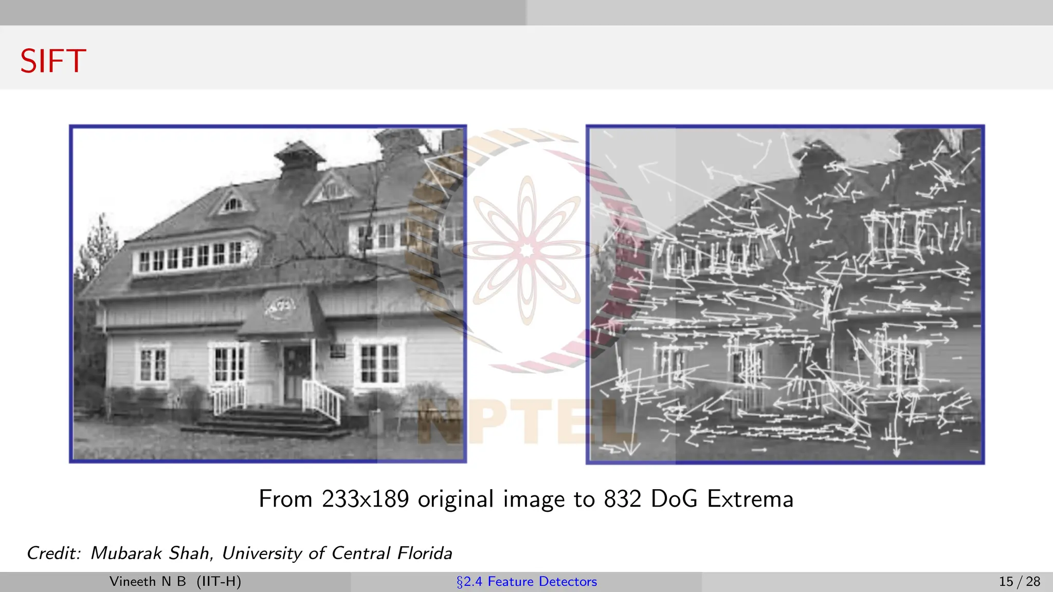
SIFT
From 233x189 originalimage to 832 DoG Extrema
Credit: Mubarak Shah, University of Central Florida
Vineeth N B (IIT-H) §2.4 Feature Detectors 15 / 28
30.
SIFT
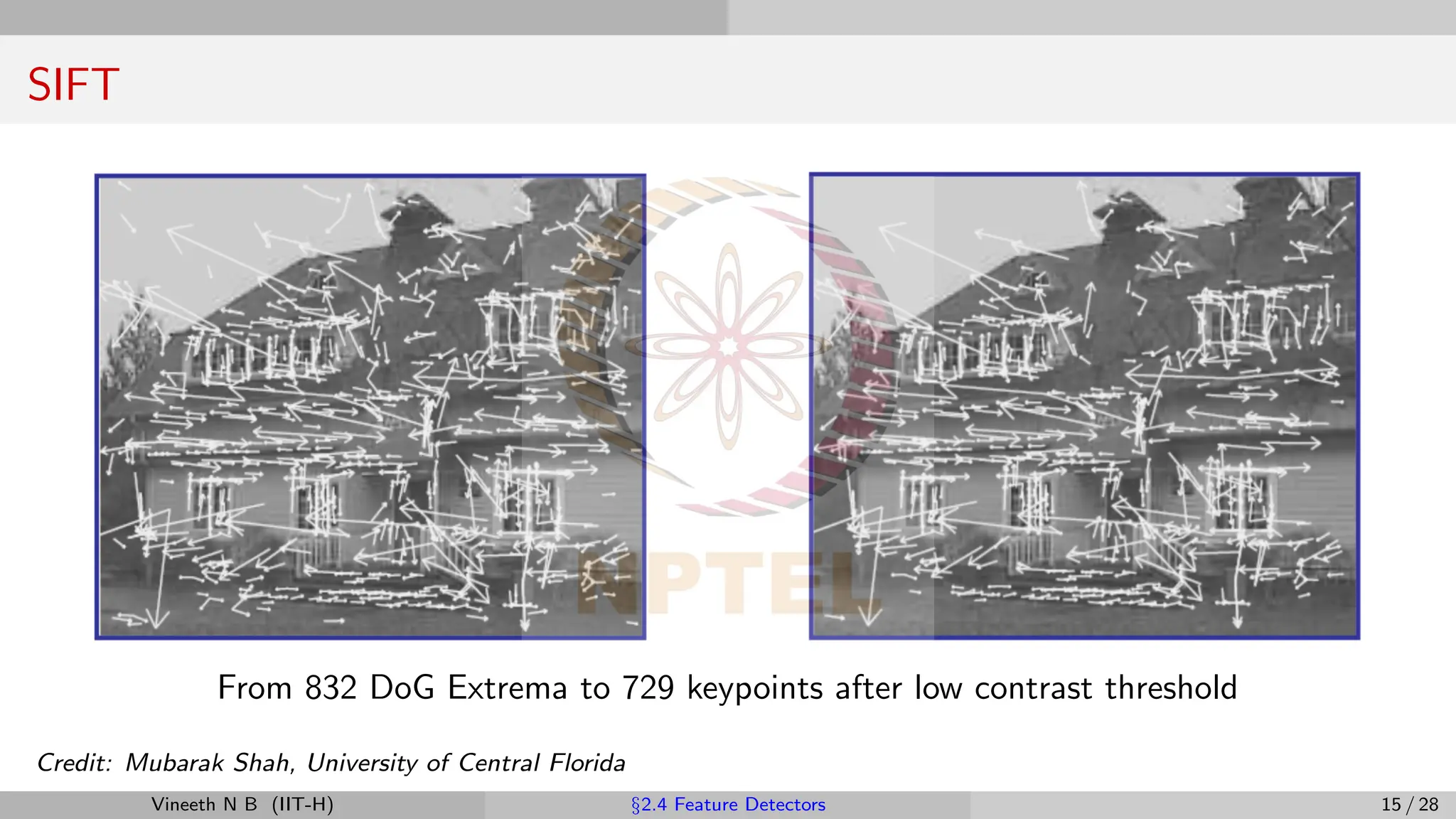
From 832 DoGExtrema to 729 keypoints after low contrast threshold
Credit: Mubarak Shah, University of Central Florida
Vineeth N B (IIT-H) §2.4 Feature Detectors 15 / 28
31.
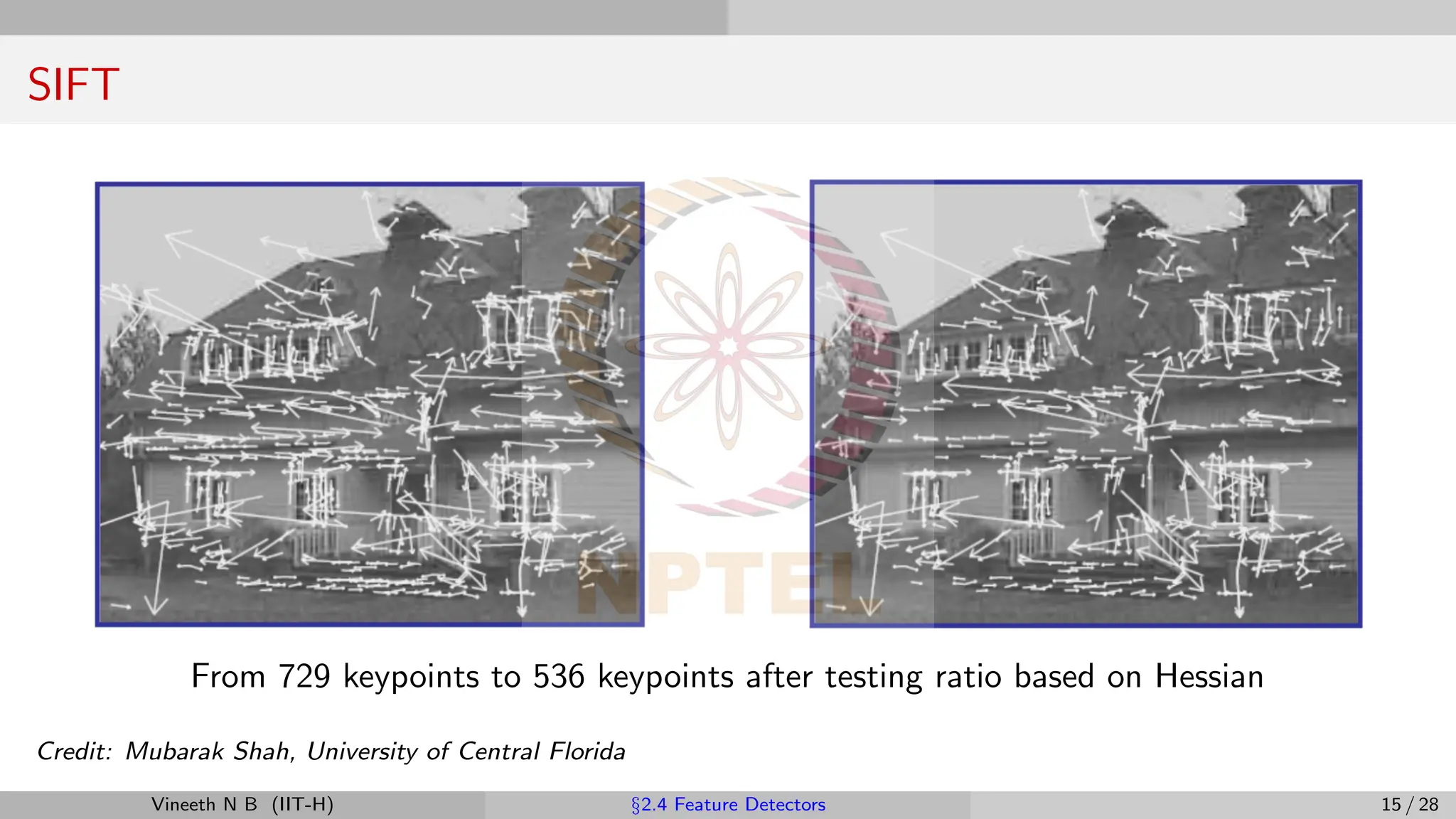
SIFT
From 729 keypointsto 536 keypoints after testing ratio based on Hessian
Credit: Mubarak Shah, University of Central Florida
Vineeth N B (IIT-H) §2.4 Feature Detectors 15 / 28
32.
SIFT Algorithm Stages
Step1: Scale-space extrema Detection - Detect interesting points (invariant to scale
and orientation) using DOG.
Step 2: Keypoint Localization - Determine location and scale at each candidate
location, and select them based on stability.
Step 3: Orientation Estimation - Use local image gradients to assign orientation to
each localized keypoint. Preserve orientation, scale and location for each feature.
Step 4: Keypoint Descriptor - Extract local image gradients at selected scale around
keypoint and form a representation invariant to local shape and illumination distortion.
Vineeth N B (IIT-H) §2.4 Feature Detectors 16 / 28
33.
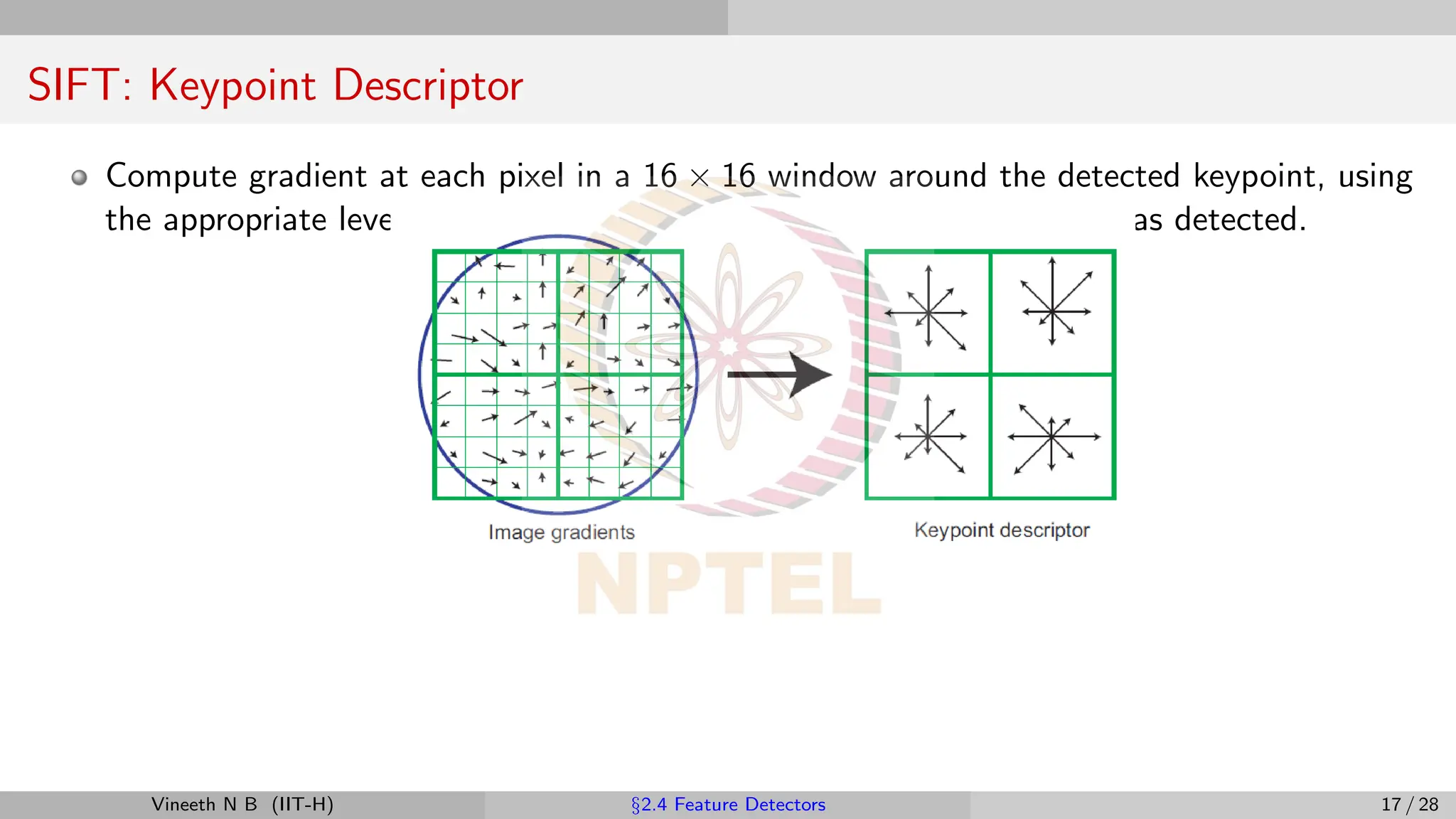
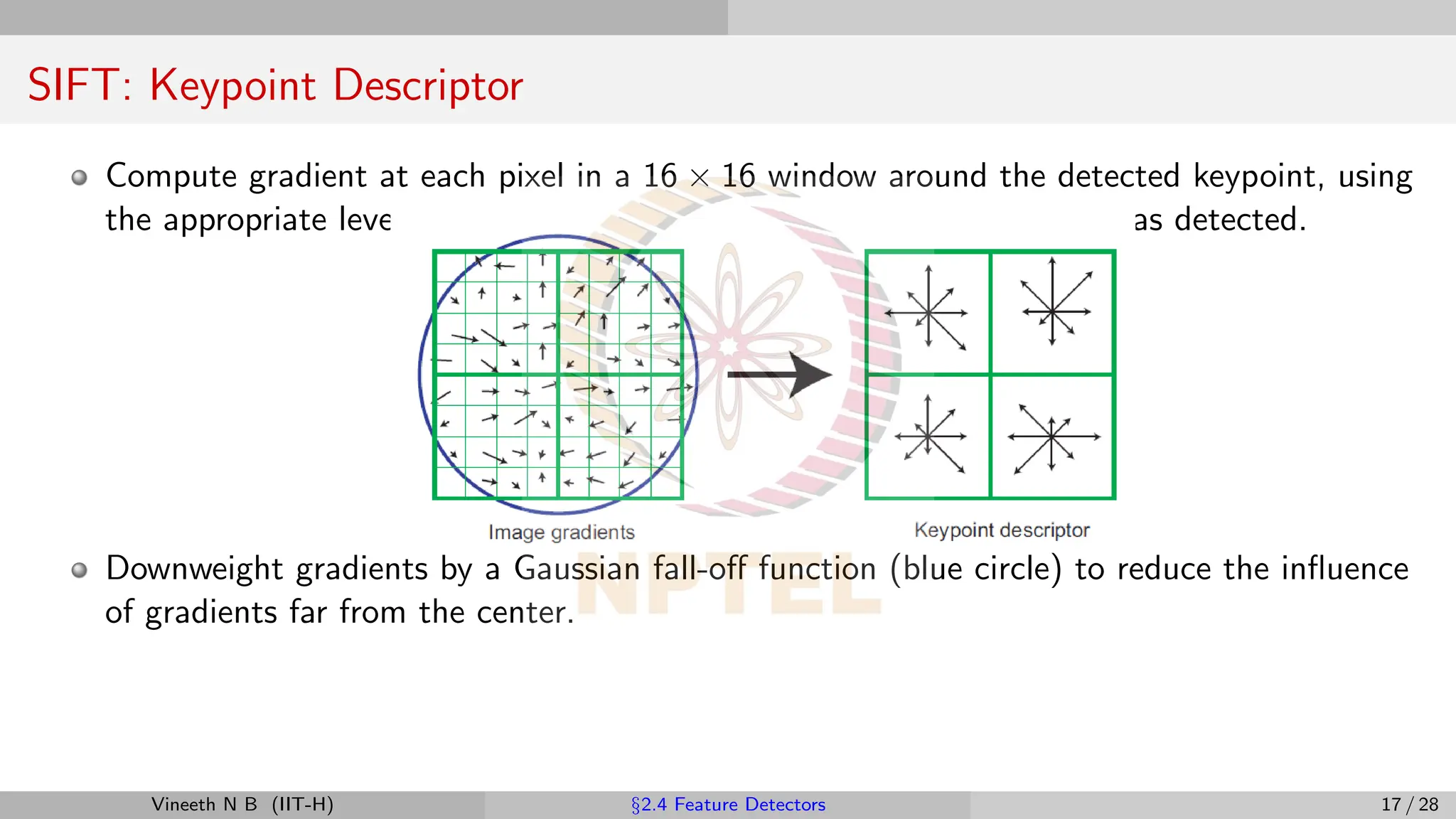
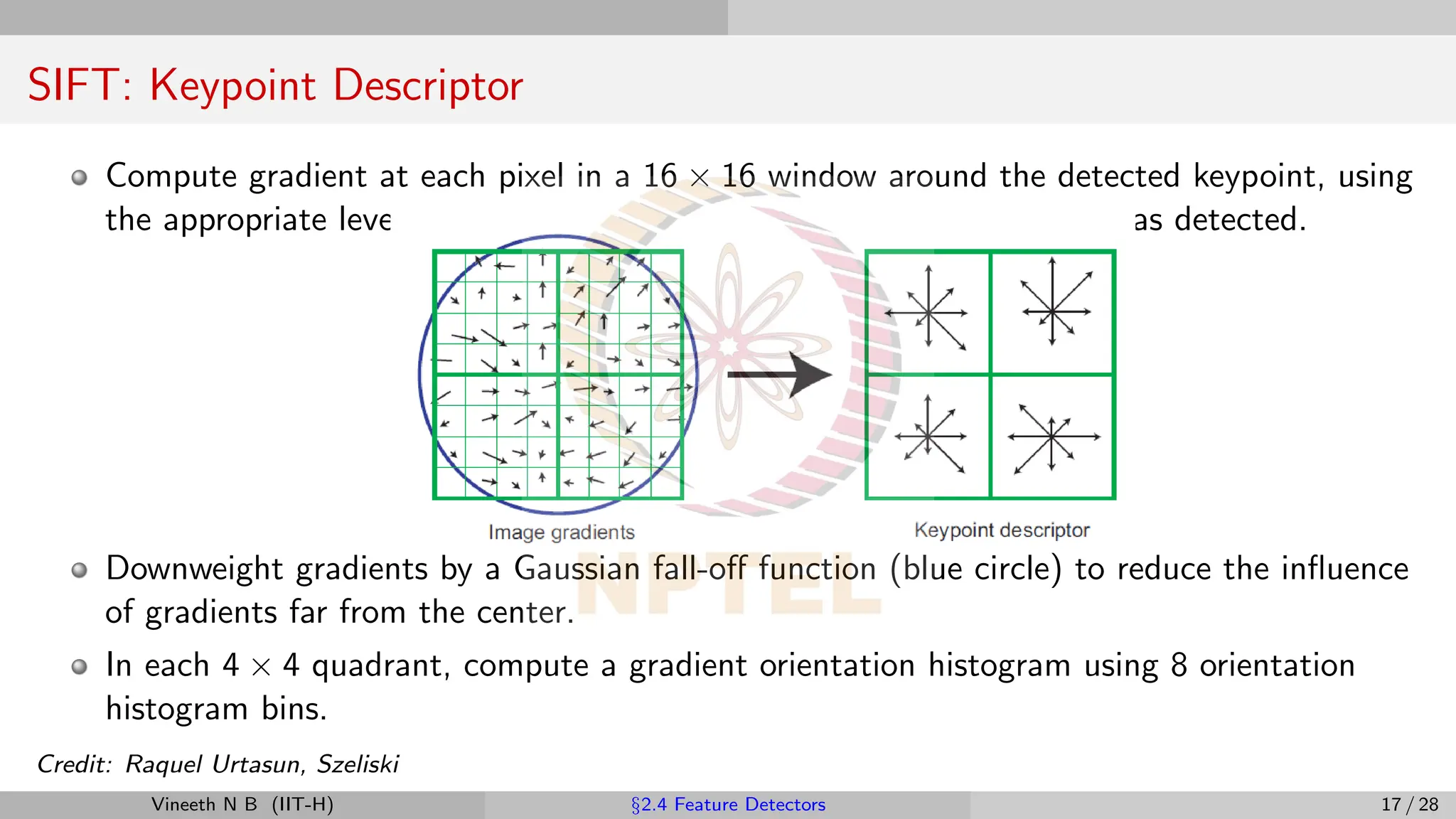
SIFT: Keypoint Descriptor
Computegradient at each pixel in a 16 × 16 window around the detected keypoint, using
the appropriate level of the Gaussian pyramid at which the keypoint was detected.
Vineeth N B (IIT-H) §2.4 Feature Detectors 17 / 28
34.
SIFT: Keypoint Descriptor
Computegradient at each pixel in a 16 × 16 window around the detected keypoint, using
the appropriate level of the Gaussian pyramid at which the keypoint was detected.
Downweight gradients by a Gaussian fall-off function (blue circle) to reduce the influence
of gradients far from the center.
Vineeth N B (IIT-H) §2.4 Feature Detectors 17 / 28
35.
SIFT: Keypoint Descriptor
Computegradient at each pixel in a 16 × 16 window around the detected keypoint, using
the appropriate level of the Gaussian pyramid at which the keypoint was detected.
Downweight gradients by a Gaussian fall-off function (blue circle) to reduce the influence
of gradients far from the center.
In each 4 × 4 quadrant, compute a gradient orientation histogram using 8 orientation
histogram bins.
Credit: Raquel Urtasun, Szeliski
Vineeth N B (IIT-H) §2.4 Feature Detectors 17 / 28
36.
SIFT: Keypoint Descriptor
Theresulting 128 non-negative values form a raw version of the SIFT descriptor vector.
To reduce the effects of contrast or gain (additive variations are already removed by the
gradient), the 128-D vector is normalized to unit length.
To further make the descriptor robust to other photometric variations, values are clipped
to 0.2 and the resulting vector is once again renormalized to unit length.
Credit: Raquel Urtasun, Szeliski
Vineeth N B (IIT-H) §2.4 Feature Detectors 18 / 28
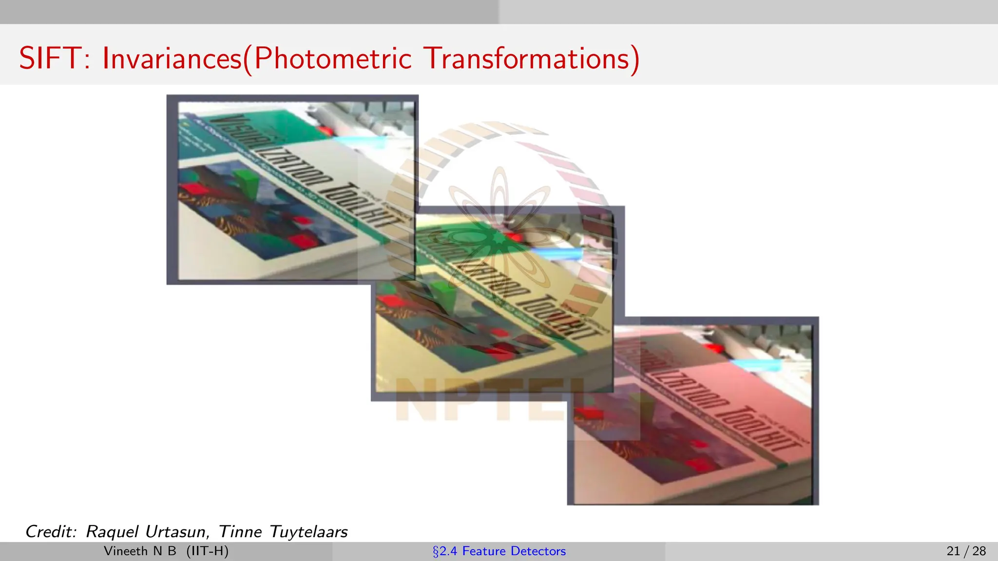
37.
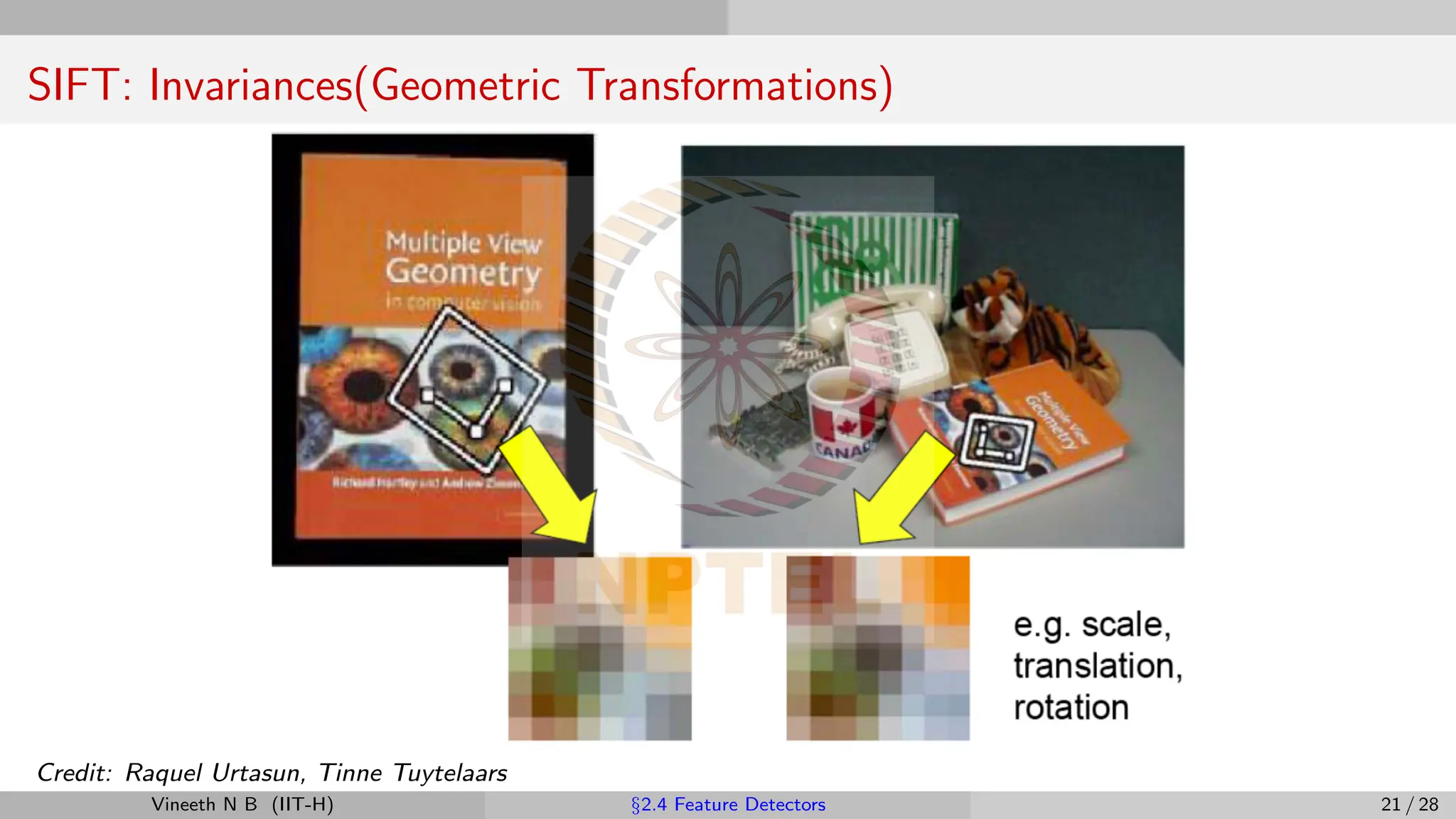
SIFT
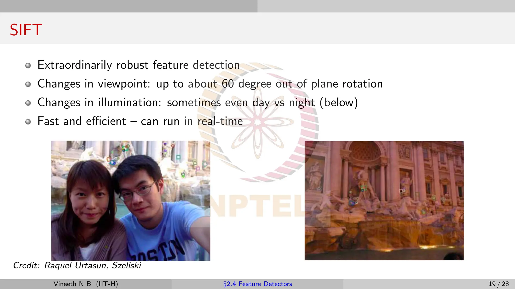
Extraordinarily robust featuredetection
Changes in viewpoint: up to about 60 degree out of plane rotation
Changes in illumination: sometimes even day vs night (below)
Fast and efficient – can run in real-time
Credit: Raquel Urtasun, Szeliski
Vineeth N B (IIT-H) §2.4 Feature Detectors 19 / 28
38.
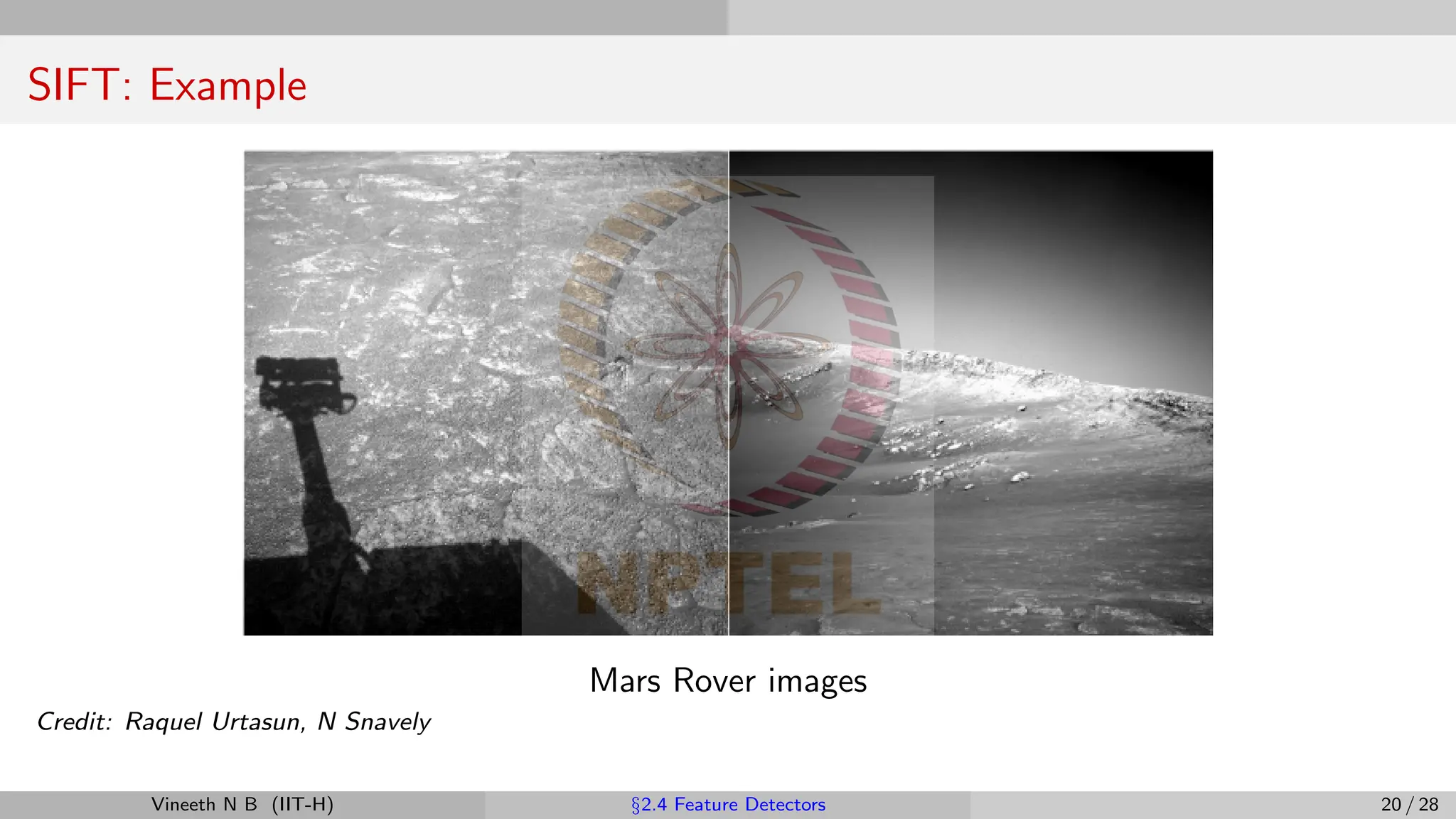
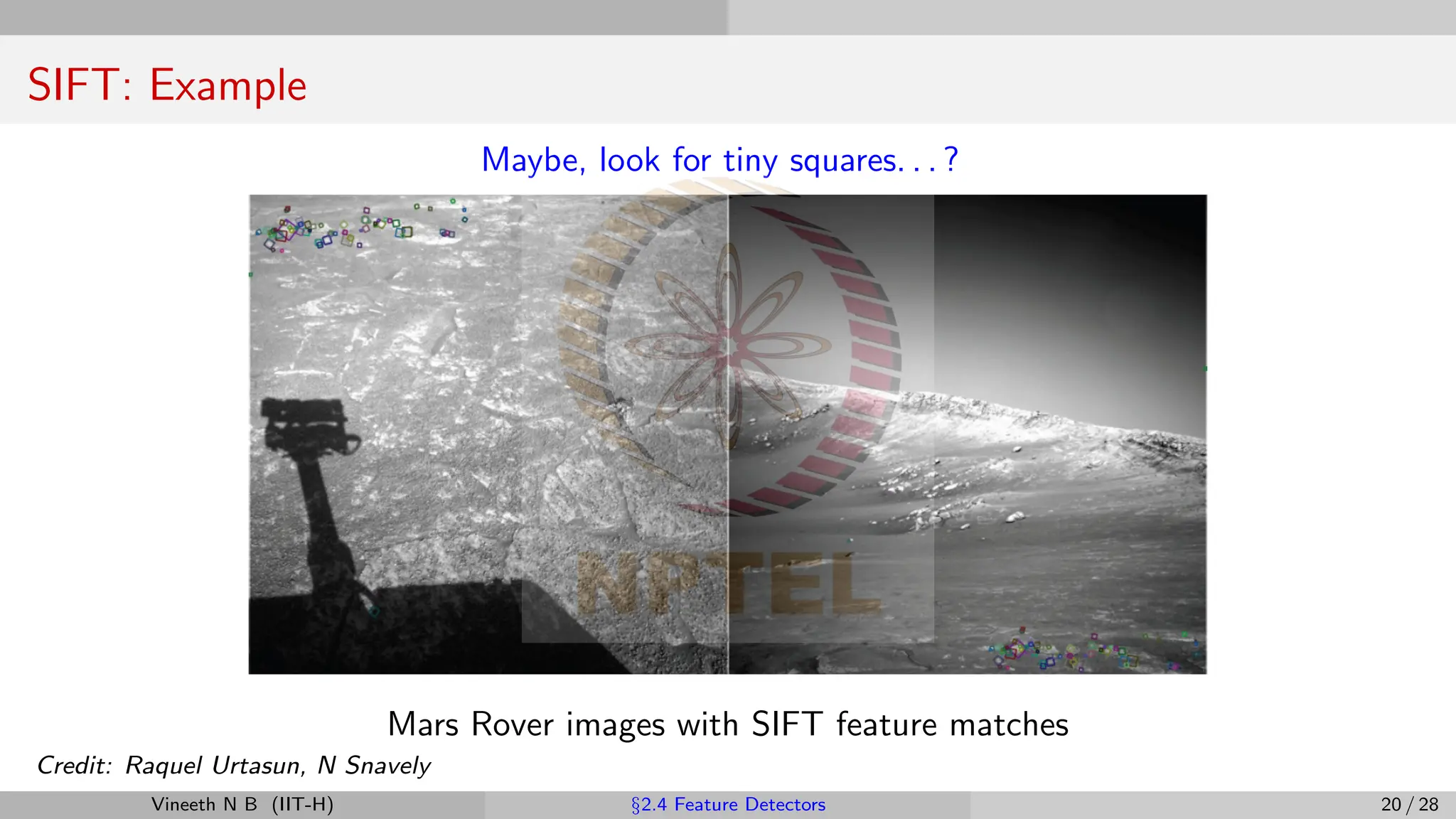
SIFT: Example
Mars Roverimages
Credit: Raquel Urtasun, N Snavely
Vineeth N B (IIT-H) §2.4 Feature Detectors 20 / 28
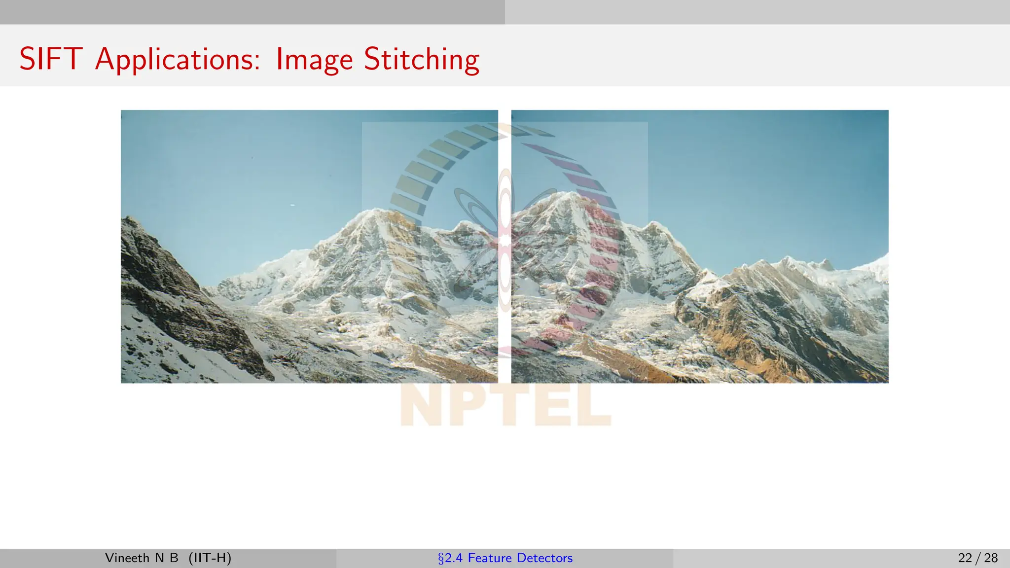
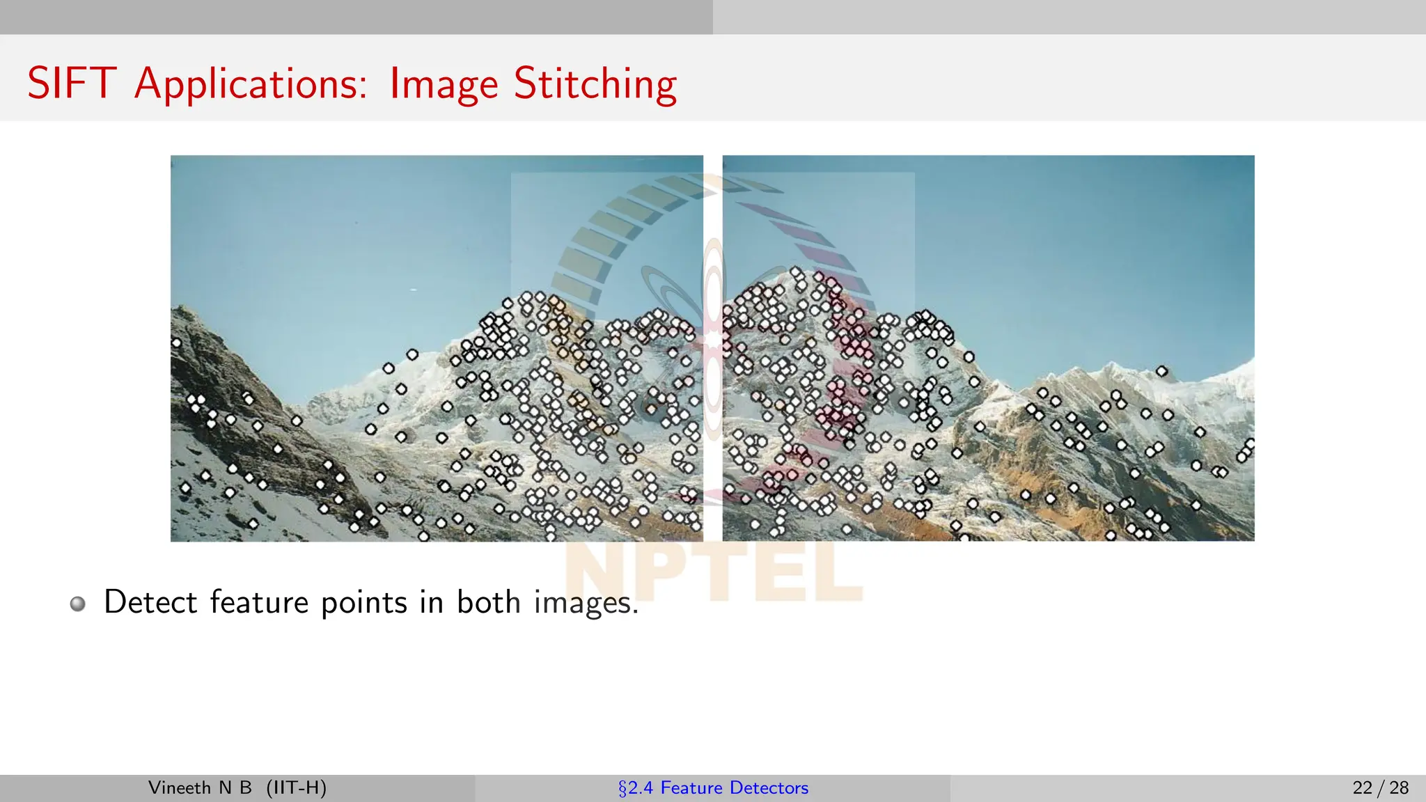
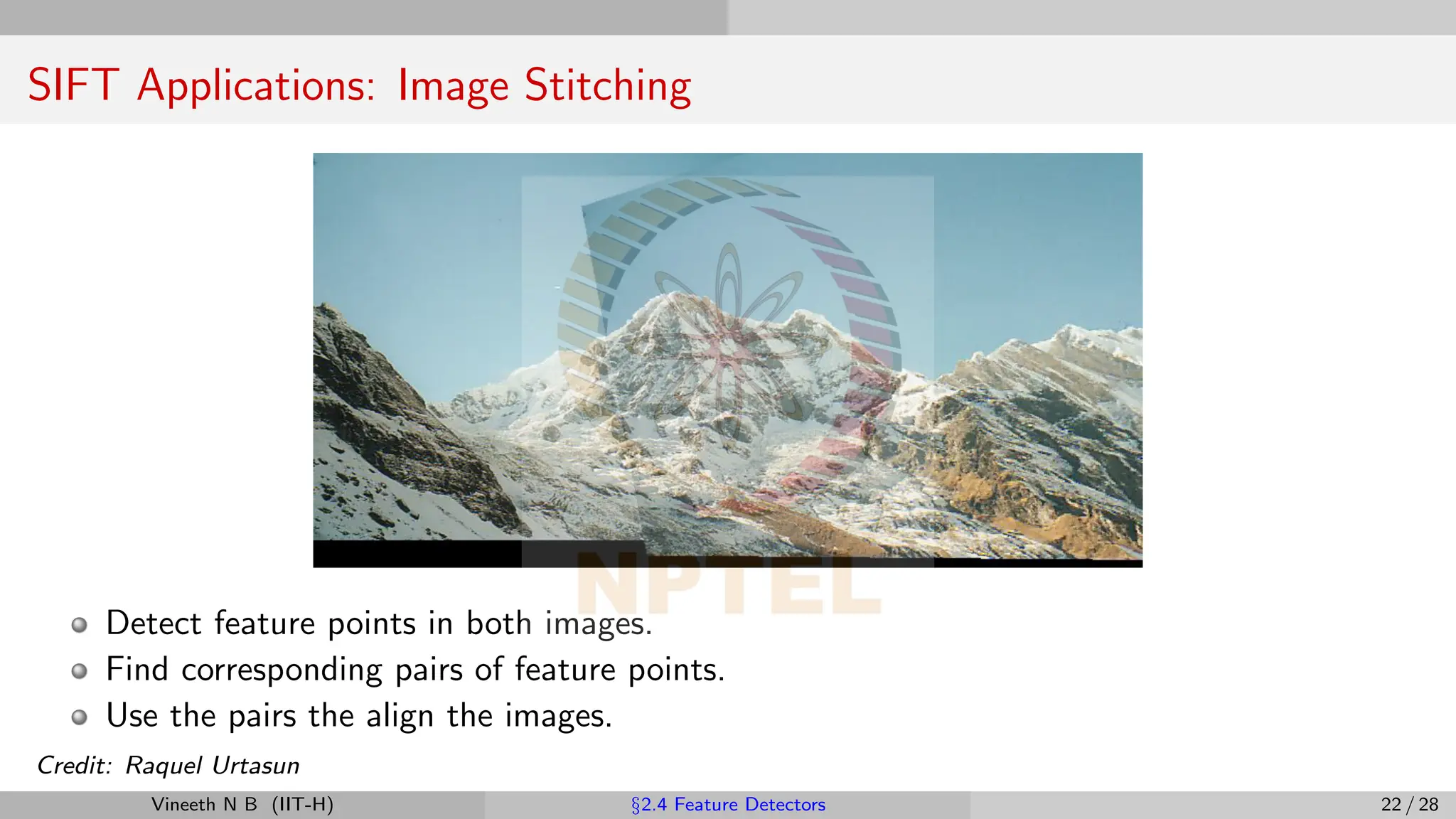
SIFT Applications: ImageStitching
Detect feature points in both images.
Vineeth N B (IIT-H) §2.4 Feature Detectors 22 / 28
45.
SIFT Applications: ImageStitching
Detect feature points in both images.
Find corresponding pairs of feature points.
Vineeth N B (IIT-H) §2.4 Feature Detectors 22 / 28
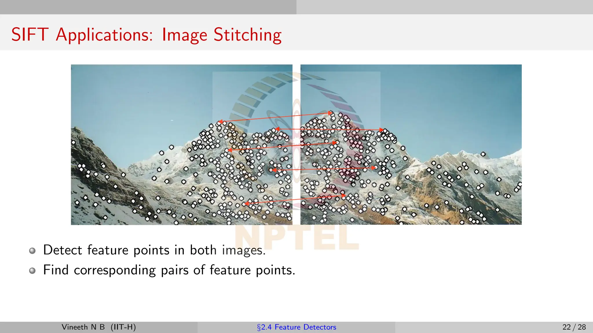
46.
SIFT Applications: ImageStitching
Detect feature points in both images.
Find corresponding pairs of feature points.
Use the pairs the align the images.
Credit: Raquel Urtasun
Vineeth N B (IIT-H) §2.4 Feature Detectors 22 / 28
47.
More Resources
If youwant to learn more on SIFT
The SIFT Keypoint Detector by David Lowe
Tutorial: SIFT (Scale-invariant feature transform)
OpenCV-Python Tutorials: Introduction to SIFT
Wikipedia: Scale-invariant feature transform
OpenSIFT: An Open-Source SIFT Library
Vineeth N B (IIT-H) §2.4 Feature Detectors 23 / 28
48.
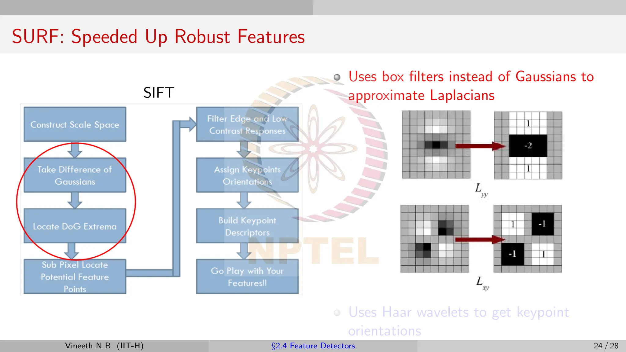
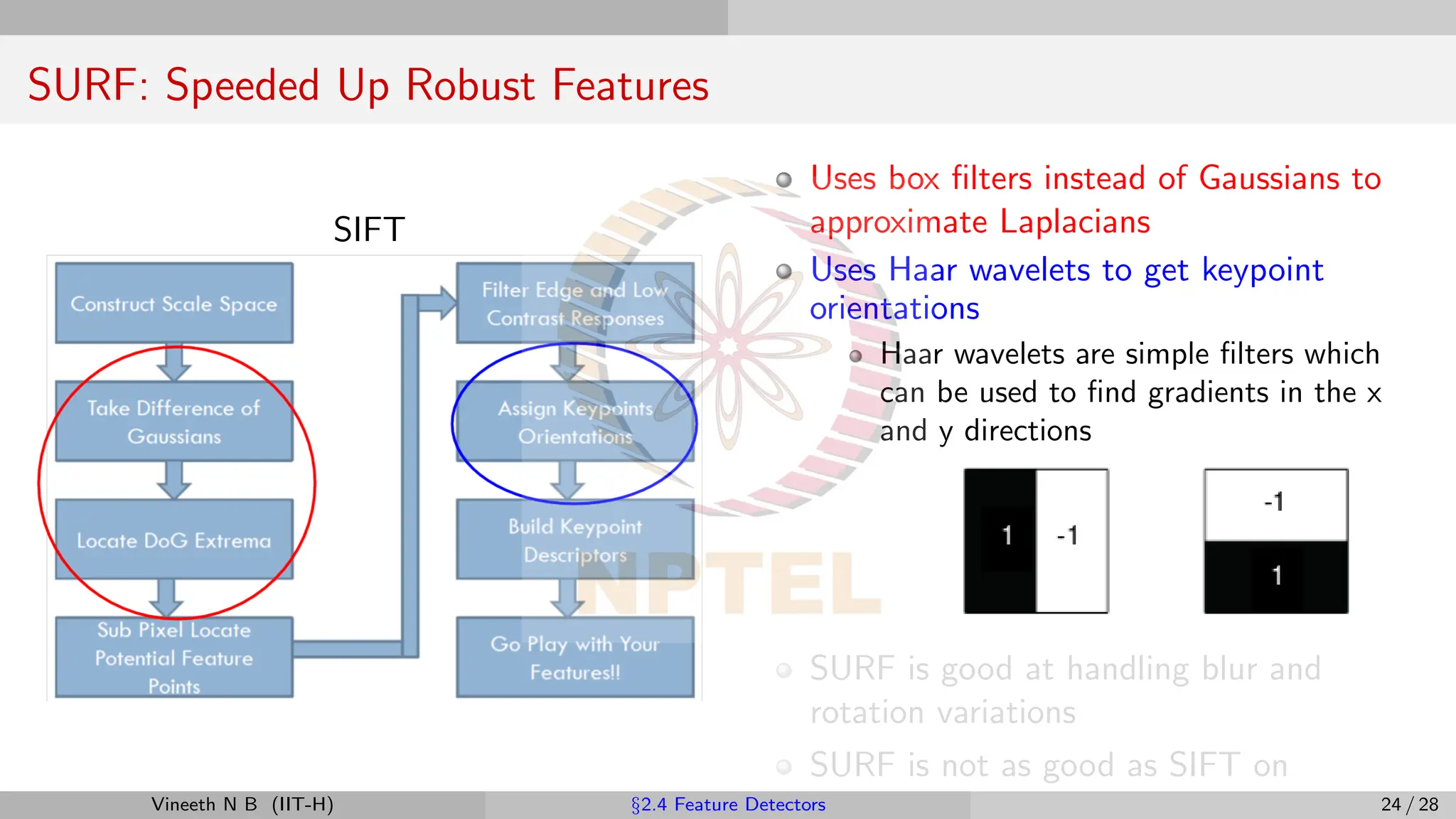
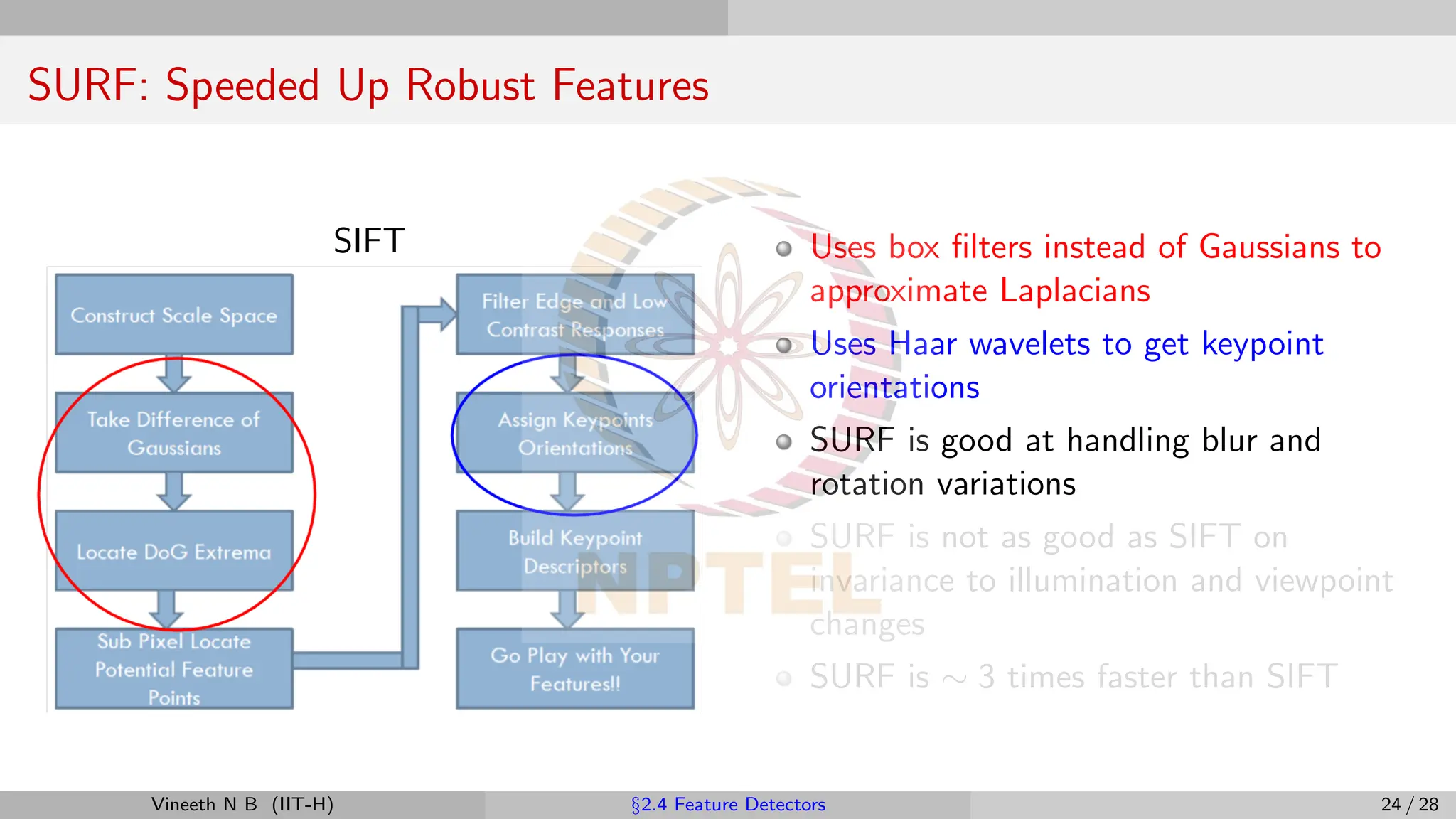
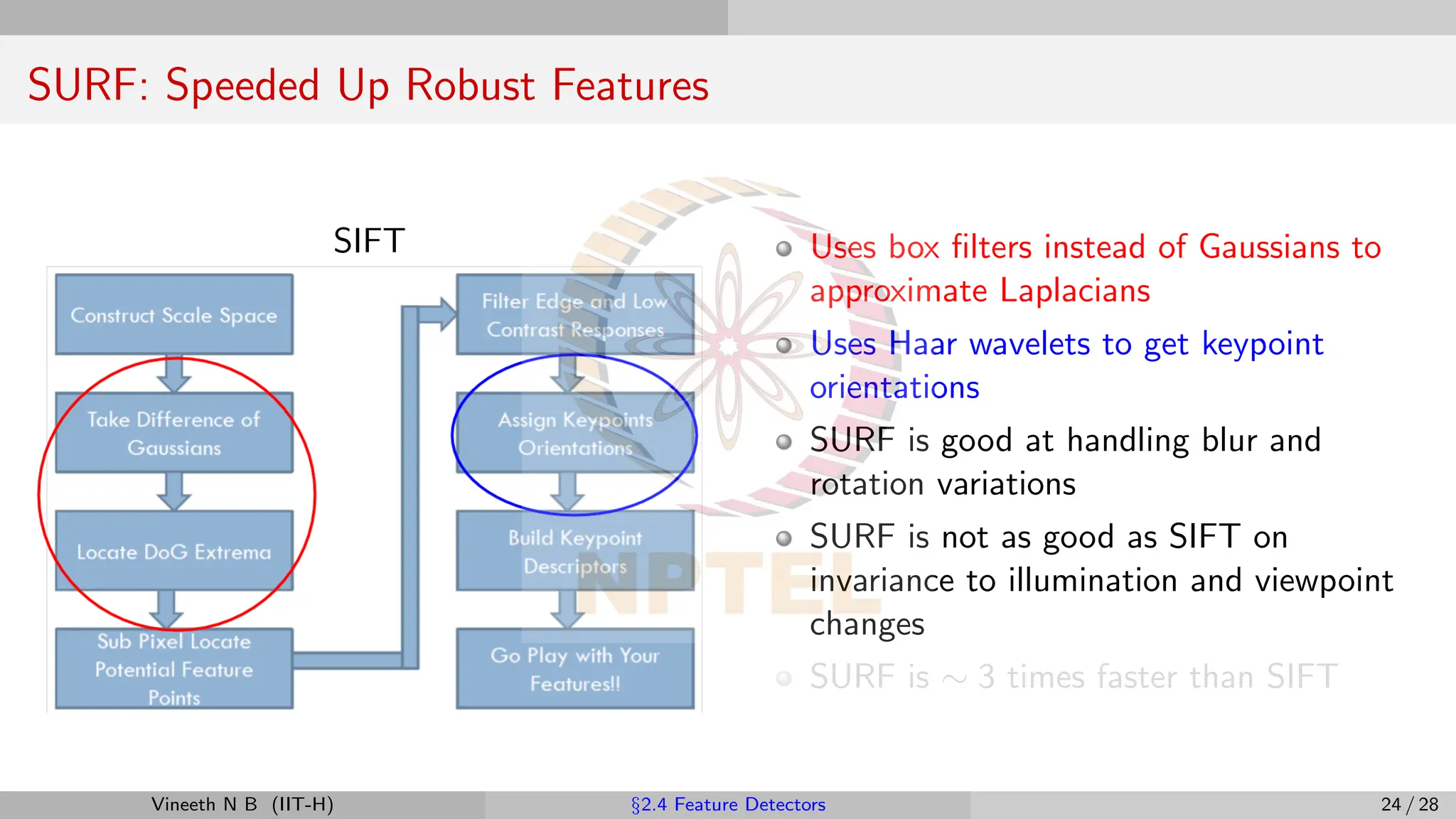
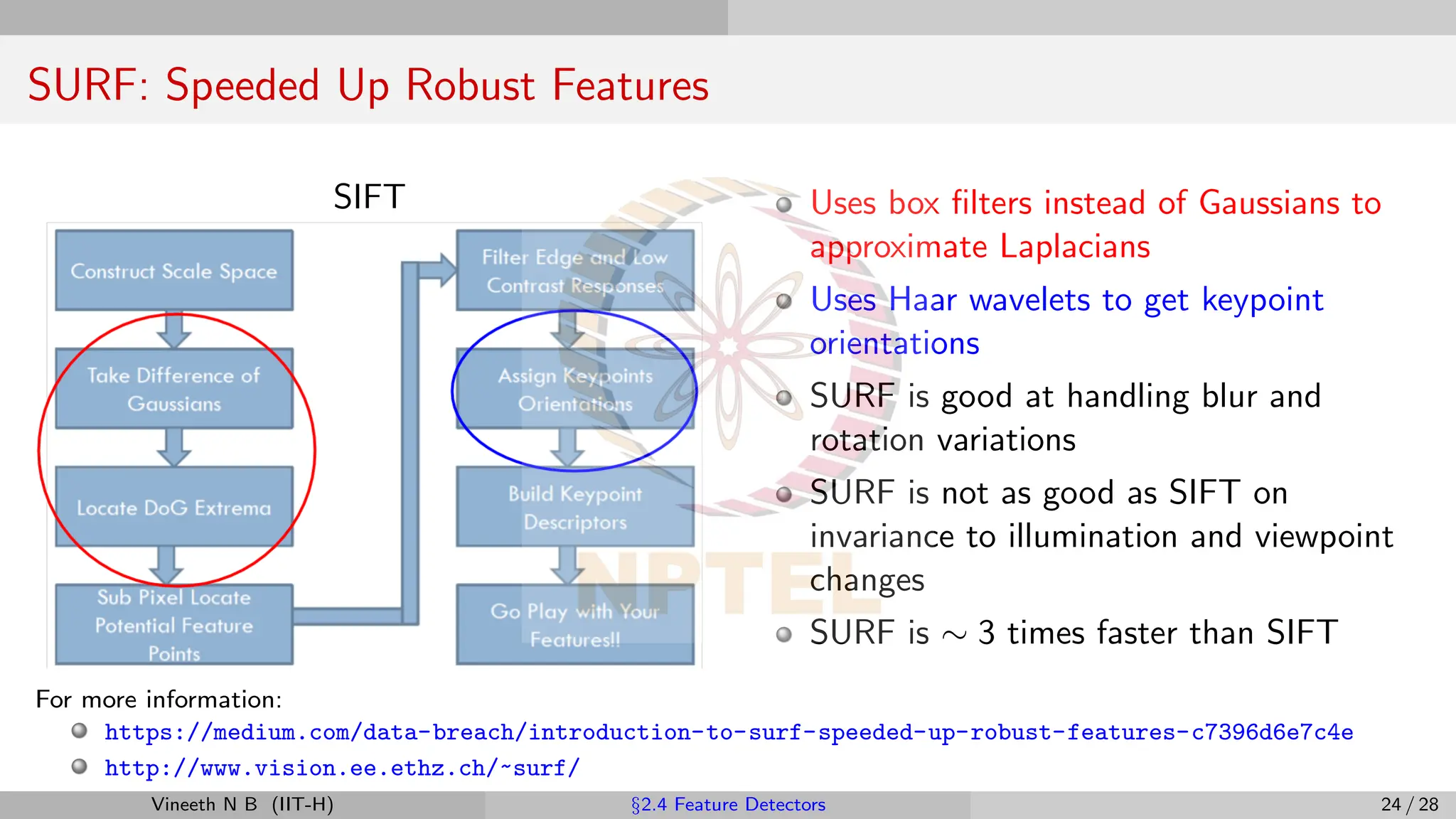
SURF: Speeded UpRobust Features
SIFT
Uses box filters instead of Gaussians to
approximate Laplacians
Uses Haar wavelets to get keypoint
orientations
Vineeth N B (IIT-H) §2.4 Feature Detectors 24 / 28
49.
SURF: Speeded UpRobust Features
SIFT
Uses box filters instead of Gaussians to
approximate Laplacians
Uses Haar wavelets to get keypoint
orientations
Haar wavelets are simple filters which
can be used to find gradients in the x
and y directions
SURF is good at handling blur and
rotation variations
SURF is not as good as SIFT on
Vineeth N B (IIT-H) §2.4 Feature Detectors 24 / 28
50.
SURF: Speeded UpRobust Features
SIFT Uses box filters instead of Gaussians to
approximate Laplacians
Uses Haar wavelets to get keypoint
orientations
SURF is good at handling blur and
rotation variations
SURF is not as good as SIFT on
invariance to illumination and viewpoint
changes
SURF is ∼ 3 times faster than SIFT
Vineeth N B (IIT-H) §2.4 Feature Detectors 24 / 28
51.
SURF: Speeded UpRobust Features
SIFT Uses box filters instead of Gaussians to
approximate Laplacians
Uses Haar wavelets to get keypoint
orientations
SURF is good at handling blur and
rotation variations
SURF is not as good as SIFT on
invariance to illumination and viewpoint
changes
SURF is ∼ 3 times faster than SIFT
Vineeth N B (IIT-H) §2.4 Feature Detectors 24 / 28
52.
SURF: Speeded UpRobust Features
SIFT Uses box filters instead of Gaussians to
approximate Laplacians
Uses Haar wavelets to get keypoint
orientations
SURF is good at handling blur and
rotation variations
SURF is not as good as SIFT on
invariance to illumination and viewpoint
changes
SURF is ∼ 3 times faster than SIFT
For more information:
https://medium.com/data-breach/introduction-to-surf-speeded-up-robust-features-c7396d6e7c4e
http://www.vision.ee.ethz.ch/~surf/
Vineeth N B (IIT-H) §2.4 Feature Detectors 24 / 28
53.
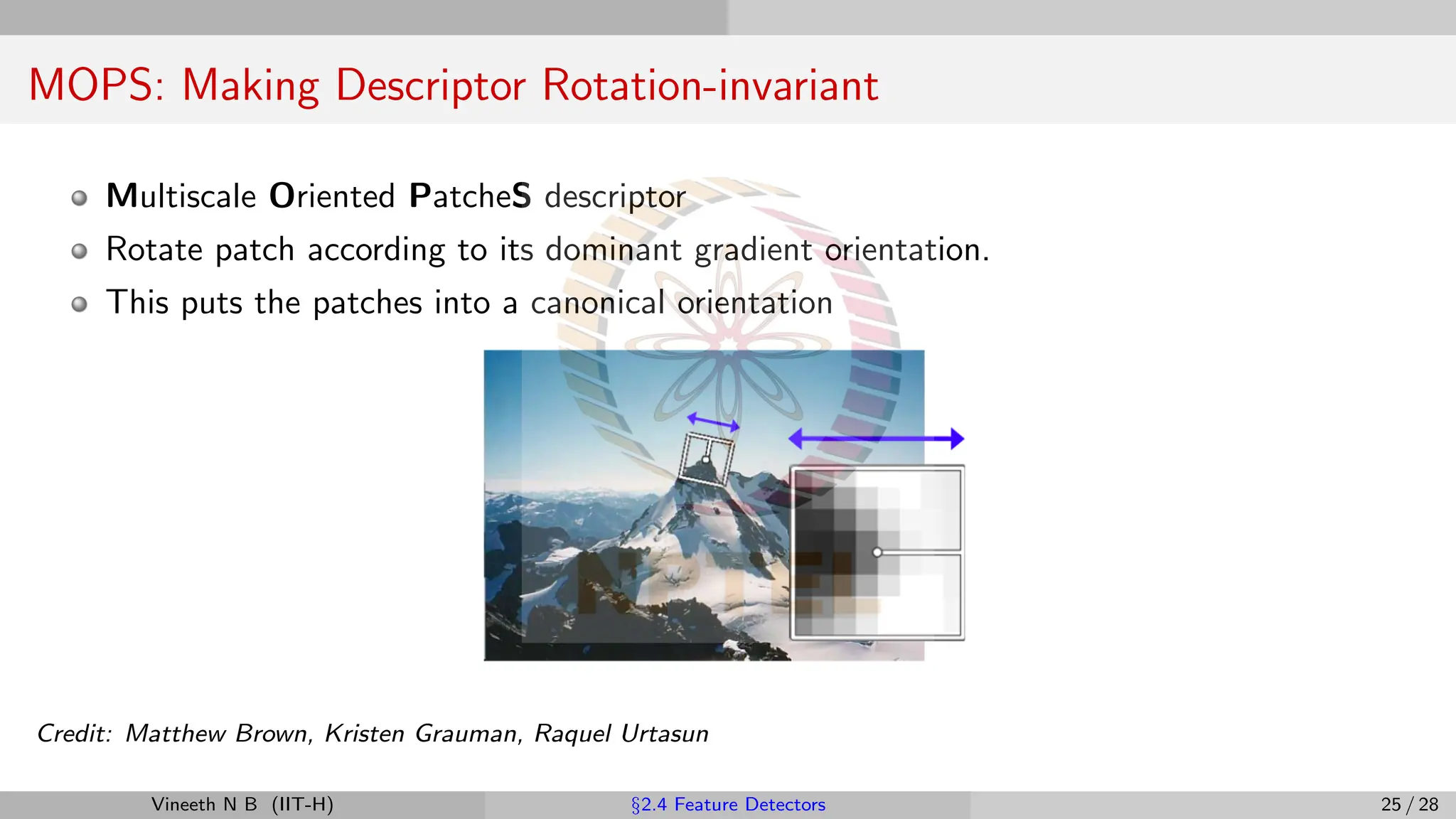
MOPS: Making DescriptorRotation-invariant
Multiscale Oriented PatcheS descriptor
Rotate patch according to its dominant gradient orientation.
This puts the patches into a canonical orientation
Credit: Matthew Brown, Kristen Grauman, Raquel Urtasun
Vineeth N B (IIT-H) §2.4 Feature Detectors 25 / 28
54.
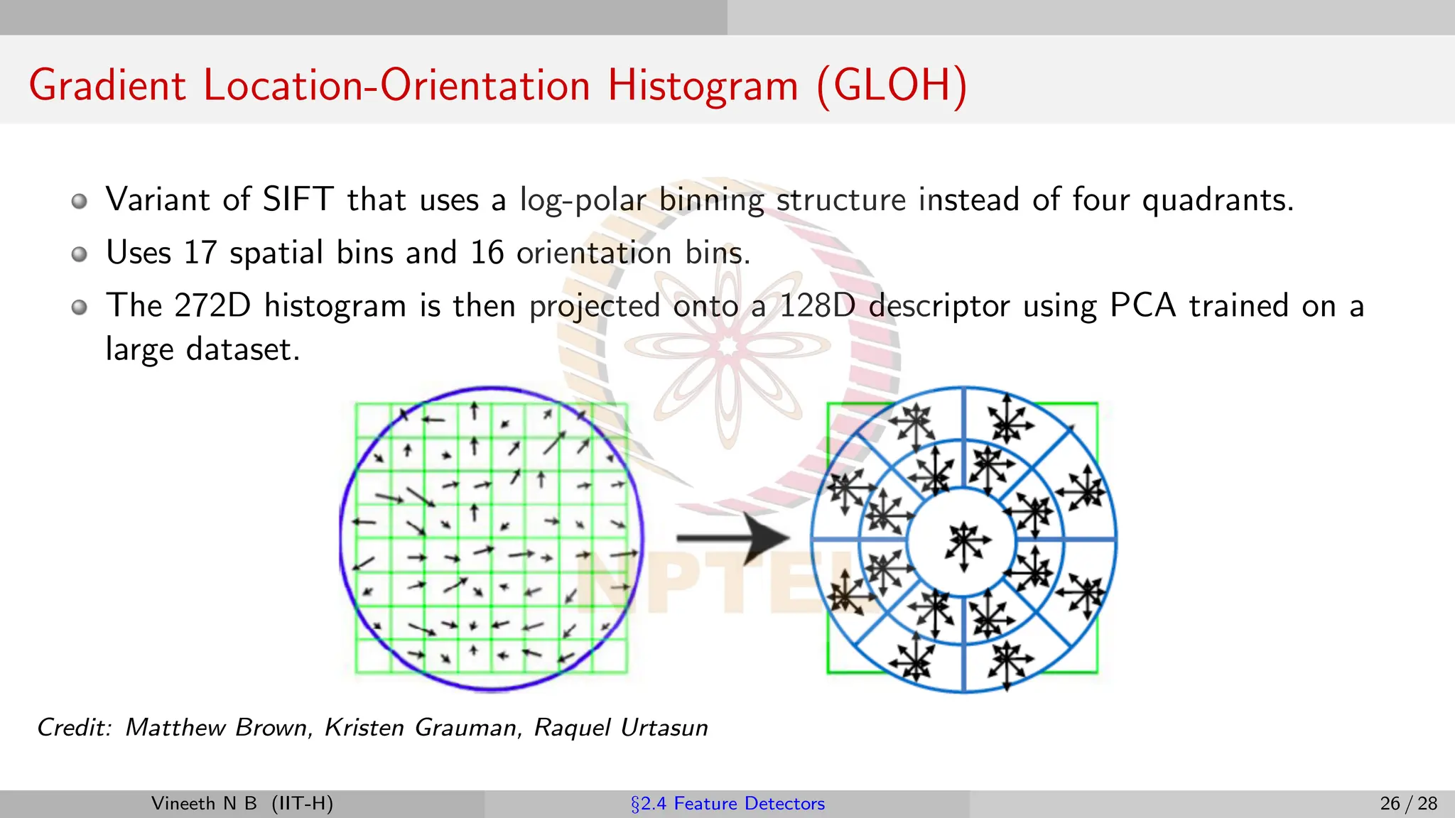
Gradient Location-Orientation Histogram(GLOH)
Variant of SIFT that uses a log-polar binning structure instead of four quadrants.
Uses 17 spatial bins and 16 orientation bins.
The 272D histogram is then projected onto a 128D descriptor using PCA trained on a
large dataset.
Credit: Matthew Brown, Kristen Grauman, Raquel Urtasun
Vineeth N B (IIT-H) §2.4 Feature Detectors 26 / 28
55.
Homework Readings
Homework
Readings
Section 3.5,Szeliski, Computer Vision: Algorithms and Applications
For more information on SURF:
OpenCV-Python Tutorials : Introduction to SURF
Wikipedia: Speeded up robust features
Multi-Scale Oriented Patches
Other links provided on respective slides
Questions
Which descriptor performs better? SIFT or MOPS?
Why is SIFT descriptor better than Harris Corner Detector?
Vineeth N B (IIT-H) §2.4 Feature Detectors 27 / 28
56.
References
References
David G. Lowe.“Distinctive Image Features from Scale-Invariant Keypoints”. In: Int. J. Comput. Vision
60.2 (Nov. 2004), 91–110.
Richard Szeliski. Computer Vision: Algorithms and Applications. Texts in Computer Science. London:
Springer-Verlag, 2011.
David Forsyth and Jean Ponce. Computer Vision: A Modern Approach. 2 edition. Boston: Pearson
Education India, 2015.
Lazebnik, Svetlana, CS 543 Computer Vision (Spring 2019). url:
https://slazebni.cs.illinois.edu/spring19/ (visited on 06/01/2020).
Shah, Mubarak, CAP 5415 - Computer Vision (Fall 2014). url:
https://www.crcv.ucf.edu/courses/cap5415-fall-2014/ (visited on 06/01/2020).
Urtasun, Raquel, Computer Vision (Winter 2013). url:
https://www.cs.toronto.edu/~urtasun/courses/CV/cv.html (visited on 06/01/2020).
Vineeth N B (IIT-H) §2.4 Feature Detectors 28 / 28

![SIFT: Keypoint Localization
The Solution:
Use Taylor series expansion of the scale-space function:
D(s0 + ∆s) = D(s0) +
∂D
∂s
T
s0
∆s +
1
2
∆sT ∂2D
∂s2 s0
∆s
where s0 = (x0, y0, σ0)T and ∆s = (δx, δy, δσ)T
The location of the extremum, ŝ, is determined by taking the derivative of this function
with respect to s and setting it to zero:
ŝ = −
∂2D
∂s2 s0
!−1
∂D
∂s s0
Next, reject low contrast points and points that lie on the edge
Low contrast points elimination:
Reject keypoint if D(ŝ) is smaller than 0.03 (assuming image values are normalized in [0,1])
Vineeth N B (IIT-H) §2.4 Feature Detectors 10 / 28](https://image.slidesharecdn.com/dl4cvweek02part04-251126072720-c9fa131c/75/DL4CV_Week02_Part04-pdfbmmmmmmbmmmmmmmmmmmm-16-2048.jpg)