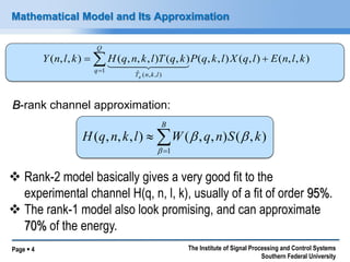
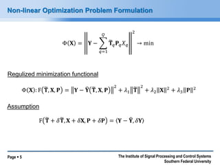
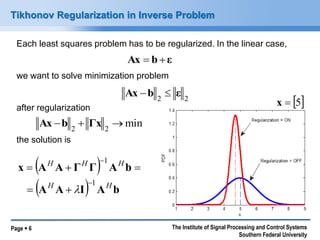
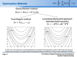
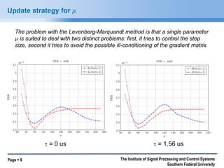
The document presents a non-linear optimization scheme for non-orthogonal multiuser access aimed at future high-capacity communication systems. It discusses the issues related to intra-cell interference and provides mathematical models to address these challenges, along with various optimization methods including Tikhonov regularization and the Levenberg-Marquardt approach. The findings indicate that significant improvements can be achieved in wireless communication systems through these optimizations and highlight future research directions.

1. Vladimir Lyashev, Mikhail Maksimov, Nikolai Merezhin
The Institute of Signal Processing and Control Systems Southern Federal University Rostov-on-Don – Taganrog, Russia
Non-Linear Optimization Scheme for Non-Orthogonal Multiuser Access
TELFOR – 2014 November 25-27, 2014

2. Page  2 The Institute of Signal Processing and Control Systems
Southern Federal University
Problem Definition
1
2
1
2
The reasons to lost orthogonality
 Birth & Death
 Channel Spread
 Low periodicity of Time Align
command – sync. problem
Future high capacity
communication systems
will require non-orthogonal
multiuser
access (METIS-2020)
Today communication systems are
based on orthogonal properties for
V-MIMO and WCDMA users.

3. Page  3
The Institute of Signal Processing and Control Systems Southern Federal University
Intra-cell Interference
Nuser = 6, td = 0 us
Nuser = 6, td = 1.56 us
Desired user
Interference
ξ
Desired user
Interference
ξ
23.7
0.11
-46 dB
14.41
4.12
-11 dB
12.52
0.67
-25 dB
11.23
2.63
-13 dB
13.37
0.95
-23 dB
16.91
1.01
-24 dB
9.83
0.65
-24 dB
2.42
3.15
2 dB
7.5
0.26
-29 dB
7.97
2.71
-9 dB
10.6
0.51
-26 dB
5.11
4.21
-1.7 dB
ETU channel (td=0us)
System model
This is equal power!

4. Page  4 The Institute of Signal Processing and Control Systems
Southern Federal University
Mathematical Model and Its Approximation
( , , ) ( , , , ) ( , ) ( , , ) ( , ) ( , , )
1
ˆ ( , , )
Y n l k H q n k l T q k P q k l X q l E n l k
Q
q
T n k l q
 


B-rank channel approximation:



B
H q n k l W q n S k
1
( , , , ) ( , , ) ( , )

 
 Rank-2 model basically gives a very good fit to the
experimental channel H(q, n, l, k), usually of a fit of order 95%.
 The rank-1 model also look promising, and can approximate
70% of the energy.

5. Page  5
The Institute of Signal Processing and Control Systems Southern Federal University
Non-linear Optimization Problem Formulation
Φ퐗=퐘− 퐓 푞퐏푞푋푞 푄 푞=12→min
Φ퐗:F퐓 ,퐗,퐏=퐘−퐘 퐓 ,퐗,퐏 2+휆1퐓 2+휆2퐗2+휆3퐏2
F퐓 +훿퐓 ,퐗+훿퐗,퐏+훿퐏=퐘−퐘 ,훿퐘
Assumption
Regulized minimization functional

6. Page  6 The Institute of Signal Processing and Control Systems
Southern Federal University
Tikhonov Regularization in Inverse Problem
2 2
Ax b  ε
Each least squares problem has to be regularized. In the linear case,
we want to solve minimization problem
after regularization
the solution is
Ax  b ε
 
A A I A b
x A A Γ Γ A b
H H
H H H
1
1


 
  

min
2 2
Ax b  Γx 
x  5

7. Page  7
The Institute of Signal Processing and Control Systems Southern Federal University
Optimization Methods
Gauss-Newton method
Φ푥=Φ푥푖+Φ′푥푖훿푥
Trust-Region method
훿푥=T(푥푖+1−푥푖)
Levenberg-Marquardt approach (damped least-squares)
훿푥=−퐉퐻퐉+휇퐈−1퐉퐻퐅
Φ퐗=퐘− 퐓 푞퐏푞푋푞 푄 푞=12→min
D. Nion and L. De Lathauwer. Levenberg-Marquardt computation of the block factor model for blind multi-user access in wireless communications.In European Signal Processing Conference (EUSIPCO), Florence, Italy, September 4-8 2006.

8. Page  8
The Institute of Signal Processing and Control Systems Southern Federal University
Update strategy for 휇
t = 1.56 us
t = 0 us
The problem with the Levenberg-Marquandt method is that a single parameter 휇 is suited to deal with two distinct problems: first, it tries to control the step size, second it tries to avoid the possible ill-conditioning of the gradient matrix.

9. Page  9 The Institute of Signal Processing and Control Systems
Southern Federal University
Convergence
0 10 20 30 40 50
-8
-7.9
-7.8
-7.7
-7.6
-7.5
-7.4
-7.3
-7.2
-7.1
-7
Iteration #
EsN0, dB
[Convergence] EsN0 for FER=10-2
the method of gradient descent
Gauss-Newton
Gauss-Newton (휇 = 0)
Gradient descent (휇 → 푖푛푓)
Fix 휇 = 60
Adaptive 휇
If Λ > 0.0,
푠푒푡 휇 <= 휇 max
1
3
, 1 − 2Λ − 1 3 ;
Otherwise,
휇 <= 2휇.
Λ푖 = Λ푖−1 + 2휇 퐻 − 퐻 푅
20 iters.

10. Page  10 The Institute of Signal Processing and Control Systems
Southern Federal University
Simulation Results
-16 -14 -12 -10 -8 -6 -4
10
-4
10
-3
10
-2
10
-1
10
0
SNR, dB
BLER
MRC w/o interference
MRC
ALS
ALS with regularization
ALS Newton
SINR before -4.77 dB -10.4 dB
SINR after

11. Page  11
The Institute of Signal Processing and Control Systems Southern Federal University
Outlook
Pilot contamination problem in massive MIMO
Fast & distributed coherent signal processing
Joint multiuser detection
Joint sector/cell
Adaptive coupling scheme for relaxation based signal processing
MU-pairing for distributed MIMO System
Complexity Reduction of Proposed Method
Conjugate gradients: CG or BiCG
Decomposition methods: waveform relaxation

12. Page  12
The Institute of Signal Processing and Control Systems Southern Federal University
THE END
Any questions ?
Vladimir Lyashev, PhD lyashev@ieee.org