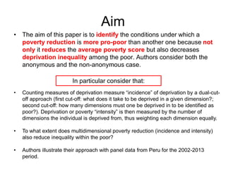
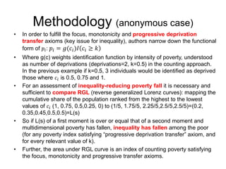
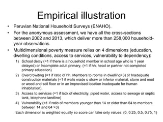
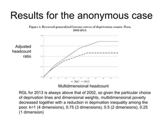
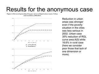
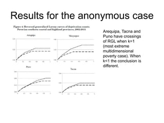
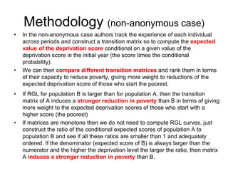
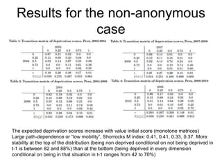
“Pro-poorest” poverty reduction 
with counting measures 
José V. Gallegos 
(Peruvian Ministry of Development and Social Inclusion) 
Gastón Yalonetzky 
(University of Leeds) 
Discussed by: 
Olga Cantó 
(Universidad de Alcalá and EQUALITAS)
Motivation 
• Pro-poorness of GDP growth largely analysed (last two decades) 
assuming that poverty can be adequately measured by a monetary 
variable and just one dimension: household disposable income 
(continuous variable to measure individual well-being). 
• Recently, clear need to connect pro-poor growth with non-monetary 
measures of well-being and multidimensional poverty indices 
(Berenger and Bresson, 2012; Ben Haj Kacem, 2013; Bonccanfuso et al, 
2009). 
• Need a framework for poverty dominance (incidence, intensity and 
inequality) for multidimensional poverty counting measures: when 
poverty indicators are not continuous (no quantile link possible) and 
number of values of poverty indicator small.
Aim 
• The aim of this paper is to identify the conditions under which a 
poverty reduction is more pro-poor than another one because not 
only it reduces the average poverty score but also decreases 
deprivation inequality among the poor. Authors consider both the 
anonymous and the non-anonymous case. 
• Counting measures of deprivation measure “incidence” of deprivation by a dual-cut-off 
approach (first cut-off: what does it take to be deprived in a given dimension?; 
second cut-off: how many dimensions must one be deprived in to be identified as 
poor?). Deprivation or poverty “intensity” is then measured by the number of 
dimensions the individual is deprived from, thus weighting each dimension equally. 
• To what extent does multidimensional poverty reduction (incidence and intensity) 
also reduce inequality within the poor? 
• Authors illustrate their approach with panel data from Peru for the 2002-2013 
period. 
In particular consider that:
Methodology (anonymous case) 
• Consider that our non-monetary poverty counting measure takes into 
account 4 well-being dimensions (d=4) for which weights are equal 
(푤푑=1/4). The deprivation score for each individual (i) would be the 
following: 
푐푖 = 
퐷 
푑=1 
푤푑 퐼 푥푖푑 < 푧푑 
• Deprivation scores can then take the values: 0, 0.25, 0.5, 0.75 and 1. 
If we were to pose a second cut-off 푘 (Alkire and Foster, 2011) then if 
푘=0.5 (2 or more dimensions) then only 3 individuals would be 
identified as multimensionally poor in this society. Authors propose an 
individual poverty measure that is: 푝푖 = 푐푖× 푘, a linear transformation 
of 푐푖 that takes values, 0, 0.125, 0.25, 0.375, 0.5. So that 4 individuals 
are deprived. 
• In this setting the author’s social poverty measure would simply be 
(symmetry, scale invariance, pop. replic. invariance, additively 
decomposable): 푃 = 
1 
푁 
푁 푝푖 
푛=1
Methodology (anonymous case) 
• In order to fulfill the focus, monotonicity and progressive deprivation 
transfer axioms (key issue for inequality), authors narrow down the functional 
form of 푝푖: 푝푖 = 푔(푐푖 )퐼 푐푖 ≥ 푘 
• Where g(c) weights identification function by intensity of poverty, understood 
as number of deprivations (deprivations=2, k=0.5) in the counting approach. 
In the previous example if k=0.5, 3 individuals would be identified as deprived 
those where 푐푖 is 0.5, 0.75 and 1. 
• For an assessment of inequality-reducing poverty fall it is necessary and 
sufficient to compare RGL (reverse generalized Lorenz curves): mapping the 
cumulative share of the population ranked from the highest to the lowest 
values of 푐푖 (1, 0.75, 0.5,0.25, 0) to (1/5, 1.75/5, 2.25/5,2.5/5,2.5/5)=(0.2, 
0.35,0.45,0.5,0.5)=L(s) 
• So if L(s) of a first moment is over or equal that of a second moment and 
multidimensional poverty has fallen, inequality has fallen among the poor 
(for any poverty index satisfying “progressive deprivation transfer” axiom, and 
for every relevant value of k). 
• Further, the area under RGL curve is an index of counting poverty satisfying 
the focus, monotonicity and progressive transfer axioms.
Empirical illustration 
• Peruvian National Household Surveys (ENAHO). 
• For the anonymous assessment, we have all the cross-sections 
between 2002 and 2013, which deliver more than 258,000 household-year 
observations 
• Multidimensional poverty measure relies on 4 dimensions (education, 
dwelling conditions, access to services, vulnerability to dependency): 
1) School delay (=1 if there is a household member in school age who is 1 year 
delayed) or Incomplete adult primary, (=1 if hh. head or partner not completed 
primary education) 
2) Overcrowding (=1 if ratio of hh. Members to rooms in dwelling>3) or Inadequate 
construction materials (=1 if walls made o straw or inferior material, stone and mud 
or wood and soil floor or in an improvised location inadequate for human 
inhabitation). 
3) Access to services (=1 if lack of electricity, piped water, access to sewage or septic 
tank, telephone landline) 
4) Vulnerability (=1 if ratio of members younger than 14 or older than 64 to members 
between 14 and 64 >3) 
Each dimension is weighted equally so score can take only values: (0, 0.25, 0.5, 0.75, 1)
Results for the anonymous case 
Adjusted 
headcount 
ratio 
Multidimensional headcount 
RGL for 2013 is always above that of 2002, so given the particular choice 
of deprivation lines and dimensional weights, multidimensional poverty 
decreased together with a reduction in deprivation inequality among the 
poor. k=1 (4 dimensions), 0.75 (3 dimensions), 0.5 (2 dimensions), 0.25 
(1 dimension)
Results for the anonymous case 
Reduction in urban 
areas was stronger 
even if the poverty 
situation in the cities 
was less serious in 
2002. Urban case 
35% reduction of RGL 
curve area A(0) while 
16.6% in rural case 
(here we consider 
poor those that lack of 
one dimension or 
more).
Results for the anonymous case 
Arequipa, Tacna and 
Puno have crossings 
of RGL when k=1 
(most extreme 
multidimensional 
poverty case). When 
k<1 the conclusion is 
different.
Methodology (non-anonymous case) 
• In the non-anonymous case authors track the experience of each individual 
across periods and construct a transition matrix so to compute the expected 
value of the deprivation score conditional on a given value of the 
deprivation score in the initial year (the score times the conditional 
probability). 
• We can then compare different transition matrices and rank them in terms 
of their capacity to reduce poverty, giving more weight to reductions of the 
expected deprivation score of those who start the poorest. 
• If RGL for population B is larger than for population A, then the transition 
matrix of A induces a stronger reduction in poverty than B in terms of giving 
more weight to the expected deprivation scores of those who start with a 
higher score (the poorest) 
• If matrices are monotone then we do not need to compute RGL curves, just 
construct the ratio of the conditional expected scores of population A to 
population B and see if all these ratios are smaller than 1 and adequately 
ordered. If the denominator (expected score of B) is always larger than the 
numerator and the higher the deprivation level the larger the ratio, then matrix 
A induces a stronger reduction in poverty than B.
Results for the non-anonymous 
case 
The expected deprivation scores increase with value initial score (monotone matrices) 
Large path-dependence or “low mobility”, Shorrocks M index: 0.41, 0.41, 0.33, 0.37. More 
stability at the top of the distribution (being non deprived conditional on not being deprived in 
t-1 is between 82 and 88%) than at the bottom (being deprived in every dimension 
conditional on being in that situation in t-1 ranges from 42 to 70%)
Results for the non-anonymous 
case 
Expected egalitarian poverty reduction 
If the initial score distributions were identical, the expected social poverty induced by matrix 1 
(2002-2004) would be lower than those produced by any other matrix (same for 2 in 
comparison to 3 and 4). The conditional distributions of expected deprivation scores 
produced before the crisis second-order dominate those during the crisis. This means that 
before the crisis (conditioned on different initial deprivation scores) the average expected 
deprivation was lower and less disperse. 
This happened even if deprivation was moving towards smaller values. This means that even 
though the distribution of poverty scores improved with a higher proportion of lower scores, 
each transition conducts somewhat less towards an egalitarian poverty reduction (a 
diminishing marginal return).
Discussion 
• There is room for motivation improvement. 
• There is room for discussion of previous literature and more explicit 
connection with related papers (this will probably ease the reading and put 
the paper in context in the current state of the art). 
• How do RGL relate to TIP curves in one-dimensional poverty 
measurement (anonymous)? Authors could comment on this, it would be 
really helpful for a better understanding of their proposal. 
• Not everybody agrees that reducing “inequality within the poor” is so 
important, in general people believe that incidence and intensity are crucial 
but inequality is less relevant. Maybe authors could comment on that. 
• How does the spurious “regression to the mean” affect your results for 
the “non-anonymous” case? We should not view that effect as pro-poor 
should we? 
Minor comments: 
Improving notation would be interesting (difficult to understand at some points). 
More explicit explanation would be useful at some points too!

Session 6 b gallegos yalonetzky

  • 1.
    “Pro-poorest” poverty reduction with counting measures José V. Gallegos (Peruvian Ministry of Development and Social Inclusion) Gastón Yalonetzky (University of Leeds) Discussed by: Olga Cantó (Universidad de Alcalá and EQUALITAS)
  • 2.
    Motivation • Pro-poornessof GDP growth largely analysed (last two decades) assuming that poverty can be adequately measured by a monetary variable and just one dimension: household disposable income (continuous variable to measure individual well-being). • Recently, clear need to connect pro-poor growth with non-monetary measures of well-being and multidimensional poverty indices (Berenger and Bresson, 2012; Ben Haj Kacem, 2013; Bonccanfuso et al, 2009). • Need a framework for poverty dominance (incidence, intensity and inequality) for multidimensional poverty counting measures: when poverty indicators are not continuous (no quantile link possible) and number of values of poverty indicator small.
  • 3.
    Aim • Theaim of this paper is to identify the conditions under which a poverty reduction is more pro-poor than another one because not only it reduces the average poverty score but also decreases deprivation inequality among the poor. Authors consider both the anonymous and the non-anonymous case. • Counting measures of deprivation measure “incidence” of deprivation by a dual-cut-off approach (first cut-off: what does it take to be deprived in a given dimension?; second cut-off: how many dimensions must one be deprived in to be identified as poor?). Deprivation or poverty “intensity” is then measured by the number of dimensions the individual is deprived from, thus weighting each dimension equally. • To what extent does multidimensional poverty reduction (incidence and intensity) also reduce inequality within the poor? • Authors illustrate their approach with panel data from Peru for the 2002-2013 period. In particular consider that:
  • 4.
    Methodology (anonymous case) • Consider that our non-monetary poverty counting measure takes into account 4 well-being dimensions (d=4) for which weights are equal (푤푑=1/4). The deprivation score for each individual (i) would be the following: 푐푖 = 퐷 푑=1 푤푑 퐼 푥푖푑 < 푧푑 • Deprivation scores can then take the values: 0, 0.25, 0.5, 0.75 and 1. If we were to pose a second cut-off 푘 (Alkire and Foster, 2011) then if 푘=0.5 (2 or more dimensions) then only 3 individuals would be identified as multimensionally poor in this society. Authors propose an individual poverty measure that is: 푝푖 = 푐푖× 푘, a linear transformation of 푐푖 that takes values, 0, 0.125, 0.25, 0.375, 0.5. So that 4 individuals are deprived. • In this setting the author’s social poverty measure would simply be (symmetry, scale invariance, pop. replic. invariance, additively decomposable): 푃 = 1 푁 푁 푝푖 푛=1
  • 5.
    Methodology (anonymous case) • In order to fulfill the focus, monotonicity and progressive deprivation transfer axioms (key issue for inequality), authors narrow down the functional form of 푝푖: 푝푖 = 푔(푐푖 )퐼 푐푖 ≥ 푘 • Where g(c) weights identification function by intensity of poverty, understood as number of deprivations (deprivations=2, k=0.5) in the counting approach. In the previous example if k=0.5, 3 individuals would be identified as deprived those where 푐푖 is 0.5, 0.75 and 1. • For an assessment of inequality-reducing poverty fall it is necessary and sufficient to compare RGL (reverse generalized Lorenz curves): mapping the cumulative share of the population ranked from the highest to the lowest values of 푐푖 (1, 0.75, 0.5,0.25, 0) to (1/5, 1.75/5, 2.25/5,2.5/5,2.5/5)=(0.2, 0.35,0.45,0.5,0.5)=L(s) • So if L(s) of a first moment is over or equal that of a second moment and multidimensional poverty has fallen, inequality has fallen among the poor (for any poverty index satisfying “progressive deprivation transfer” axiom, and for every relevant value of k). • Further, the area under RGL curve is an index of counting poverty satisfying the focus, monotonicity and progressive transfer axioms.
  • 6.
    Empirical illustration •Peruvian National Household Surveys (ENAHO). • For the anonymous assessment, we have all the cross-sections between 2002 and 2013, which deliver more than 258,000 household-year observations • Multidimensional poverty measure relies on 4 dimensions (education, dwelling conditions, access to services, vulnerability to dependency): 1) School delay (=1 if there is a household member in school age who is 1 year delayed) or Incomplete adult primary, (=1 if hh. head or partner not completed primary education) 2) Overcrowding (=1 if ratio of hh. Members to rooms in dwelling>3) or Inadequate construction materials (=1 if walls made o straw or inferior material, stone and mud or wood and soil floor or in an improvised location inadequate for human inhabitation). 3) Access to services (=1 if lack of electricity, piped water, access to sewage or septic tank, telephone landline) 4) Vulnerability (=1 if ratio of members younger than 14 or older than 64 to members between 14 and 64 >3) Each dimension is weighted equally so score can take only values: (0, 0.25, 0.5, 0.75, 1)
  • 7.
    Results for theanonymous case Adjusted headcount ratio Multidimensional headcount RGL for 2013 is always above that of 2002, so given the particular choice of deprivation lines and dimensional weights, multidimensional poverty decreased together with a reduction in deprivation inequality among the poor. k=1 (4 dimensions), 0.75 (3 dimensions), 0.5 (2 dimensions), 0.25 (1 dimension)
  • 8.
    Results for theanonymous case Reduction in urban areas was stronger even if the poverty situation in the cities was less serious in 2002. Urban case 35% reduction of RGL curve area A(0) while 16.6% in rural case (here we consider poor those that lack of one dimension or more).
  • 9.
    Results for theanonymous case Arequipa, Tacna and Puno have crossings of RGL when k=1 (most extreme multidimensional poverty case). When k<1 the conclusion is different.
  • 10.
    Methodology (non-anonymous case) • In the non-anonymous case authors track the experience of each individual across periods and construct a transition matrix so to compute the expected value of the deprivation score conditional on a given value of the deprivation score in the initial year (the score times the conditional probability). • We can then compare different transition matrices and rank them in terms of their capacity to reduce poverty, giving more weight to reductions of the expected deprivation score of those who start the poorest. • If RGL for population B is larger than for population A, then the transition matrix of A induces a stronger reduction in poverty than B in terms of giving more weight to the expected deprivation scores of those who start with a higher score (the poorest) • If matrices are monotone then we do not need to compute RGL curves, just construct the ratio of the conditional expected scores of population A to population B and see if all these ratios are smaller than 1 and adequately ordered. If the denominator (expected score of B) is always larger than the numerator and the higher the deprivation level the larger the ratio, then matrix A induces a stronger reduction in poverty than B.
  • 11.
    Results for thenon-anonymous case The expected deprivation scores increase with value initial score (monotone matrices) Large path-dependence or “low mobility”, Shorrocks M index: 0.41, 0.41, 0.33, 0.37. More stability at the top of the distribution (being non deprived conditional on not being deprived in t-1 is between 82 and 88%) than at the bottom (being deprived in every dimension conditional on being in that situation in t-1 ranges from 42 to 70%)
  • 12.
    Results for thenon-anonymous case Expected egalitarian poverty reduction If the initial score distributions were identical, the expected social poverty induced by matrix 1 (2002-2004) would be lower than those produced by any other matrix (same for 2 in comparison to 3 and 4). The conditional distributions of expected deprivation scores produced before the crisis second-order dominate those during the crisis. This means that before the crisis (conditioned on different initial deprivation scores) the average expected deprivation was lower and less disperse. This happened even if deprivation was moving towards smaller values. This means that even though the distribution of poverty scores improved with a higher proportion of lower scores, each transition conducts somewhat less towards an egalitarian poverty reduction (a diminishing marginal return).
  • 13.
    Discussion • Thereis room for motivation improvement. • There is room for discussion of previous literature and more explicit connection with related papers (this will probably ease the reading and put the paper in context in the current state of the art). • How do RGL relate to TIP curves in one-dimensional poverty measurement (anonymous)? Authors could comment on this, it would be really helpful for a better understanding of their proposal. • Not everybody agrees that reducing “inequality within the poor” is so important, in general people believe that incidence and intensity are crucial but inequality is less relevant. Maybe authors could comment on that. • How does the spurious “regression to the mean” affect your results for the “non-anonymous” case? We should not view that effect as pro-poor should we? Minor comments: Improving notation would be interesting (difficult to understand at some points). More explicit explanation would be useful at some points too!