This document provides a cheat sheet on vector and matrix operations, time series analysis functions, modeling functions, and plotting functions in R. It includes the basic syntax for constructing and selecting vectors and matrices, as well as functions for time series decomposition, modeling, testing, and plotting time series data. Examples are given for accessing Quandl data and plotting it using ggplot2.

1. 1 www.quandl.com
R Cheat Sheet
Vector and Matrix Operations
Construction
c()
cbind()
rbind()
matrix()
Concatenate
Column Concatenate
Row Concatenate
Create matrix
v <- c(1,2,3,4) # 1 2 3 4
cbind(v,v) # 2 Columns
rbind(v,v) # 2 Rows
mat <- matrix(v,nrow=2,ncol=2)
Selection
v[1]
tail(v,1)
mat[2,1]
mat[1,]
mat[,2]
v[c(1,3)]
v[-c(1,3)]
mat[,c(1,2)]
mat[,1:5]
mat[,“col”]
Utility
length()
dim()
sort()
order()
names()
Length of vector
Dimensions of vector/matrix/dataframe
Sorts vector
Index to sort vector e.g. sort(v) == v[order(v)]
Names of columns
Select first
Select last
Select row 2, column 1
Select row 1
Select column 2
Select the first and third values
Select all but the first and third values
Select columns 1 and 2
Select columns 1 to 5
Select column named “col”
Basic Syntax
#
<- or =
<<-
v[1]
*
%*%
/
%/%
%%
Comments
Assignment
Global Assignment
First element in a vector
Scalar Multiplication
Matrix Multiplication
Division
Integer Division
Remainder
# This is not interpreted
a <- 1; b = 2
a <<- 10 # Not recommended
v[1]
c(1,1)*c(1,1) # 1 1
c(1,1)%*%c(1,1) # 2
1/2 # 0.5
1%/%2 # 0
7%%6 # 1
Example

2. 2 www.quandl.com
Time Series
Time Series Classes
ts(data, frequency)
zoo(data, index)
xts(data, index)
tis()
irts()
timeSeries()
Structures
data.frame(…)
list(name=var)
ts(data, frequency)
Tests The package tseries is required for a most of these functions
adf.test
jarque.bera.test
kpss.test
po.test
pp.test
runs.test
terasvirta.test
white.test
box.test
From R base, handles regularly spaced time series
Part of the zoo package, handles irregularily spaced data using arbitrary time
date classes
Modification to zoo, gives more power to selecting date subsets
Uses POSIXct time stamps
From the package tseries and uses POSIXct time stamps
Uses timeDate time stamps
Computes the Augmented Dickey-Fuller test for the null that the series
has a unit root
Tests the null of normaility for the series using the Jarque-Bera test statistics
Computes the KPSS test for the null that the series is level or trend stationary
Computes the Phillips-Ouliaris test for the null that the series in not cointegrated
Computes the Phillips-Perron test for the null that the series has a unit root
Computes the runs test for randomness of the binary series
Generically computes Teraesvirta’s neural network test for neglected
nonlinearity for the time series
Generically computes the White neural network test for neglected
nonlinearity for the time series
Compute the Box-Pierce or Ljung-Box test statistics for examining the null of independence
in a given series
Takes multiple variables with the same number of rows and creates a dataframe
R’s implementation of a hash, takes multiple variables or variable tag pairs
Creates a regularly spaced time series object
Apply
apply(data, axis, fun)
lapply(data, fun)
tapply(data, index, fun)
I/O
read.table(“filename”, sep=”,”)
read.csv()
fromJSON()
xmlTreeParse()
write.csv()
Apply the function fun to data along axis
Apply the function fun to the list or vector data
Apply the function fun to data along the list of factors index
Reads information in from file with a variable delimiter
Read csv file into dataframe
Read JSON formatted file or string into a list - Requires RJSONIO
Read XML formatted file or string into a list - Requires XML
Writes a dataframe or matrix (or tries to convert input to one) and writes to csv
For a great introduction to using apply see this article.

3. 3 www.quandl.com
Quandl is a search engine for numerical data, alowing easy
access to financial, social, and demographic data from
hundreds of sources.
Quandl
The Quandl package enables Quandl API access from
within R which makes acquiring and manipulating
numerical data as quick and easy as possible. In your
first Quandl function call you should specifiy your
authtoken (found on Quandl’s website after signing up)
to avoid certain API call limits.
See www.quandl.com/help/packages/R for more.
Models The package forecast is required for some of these functions
ar()
ma()
arima()
auto.arima()
ets()
HoltWinters()
forecast(model, n)
Utility
index()
coredata()
lag(ts, n)
diff(ts, n)
acf() or Acf()
pacf() or Pacf()
ndiff()
accuracy()
Fits an autoregressive model
Fits a simple moving average model
Fits an arima model with specified parameters
Automatically fits an arima model
Fits an exponential smoothing model
Computes Holt-Winters Filtering of a given time series
Forecasts the next n points from the time series model
Returns the index (dates) of the time series
Returns a matrix of data from the time series sans index
Returns the time series shifted n times
Returns the time series differences n times
Returns the autocorrelation function of the time series (Acf() from the forecast package)
Returns the partial autocorrelation function of the time series (Pacf() from the
forecast package)
Returns the number of differences needed for a time series to have stationarity
Computes the accuracy of a time series model
Decomposition
decompose()
filter()
stl()
Decompoes the series into seasonal, trend and irregular components using moving averages
Applies a linear filter to a series
Decomposes the series into seasonal, trend and irregular components using loess methods
shapiro.test
ks.test
punitroot
Test for normality
Test for specified distribution
Computes the cumulative probability of MacKinnon’s unit root tes statistic
Quandl.auth(“AUTHETICATION_TOKEN”)
Quandl(“QUANDL/CODE”)
Quandl.search(“query”)
Call this first to increase your daily limit
Download Quandl data for a certain Quandl code as a data frame
Search Quandl. Prints first three outputs to screen, returns all in a list.

4. 4 www.quandl.com
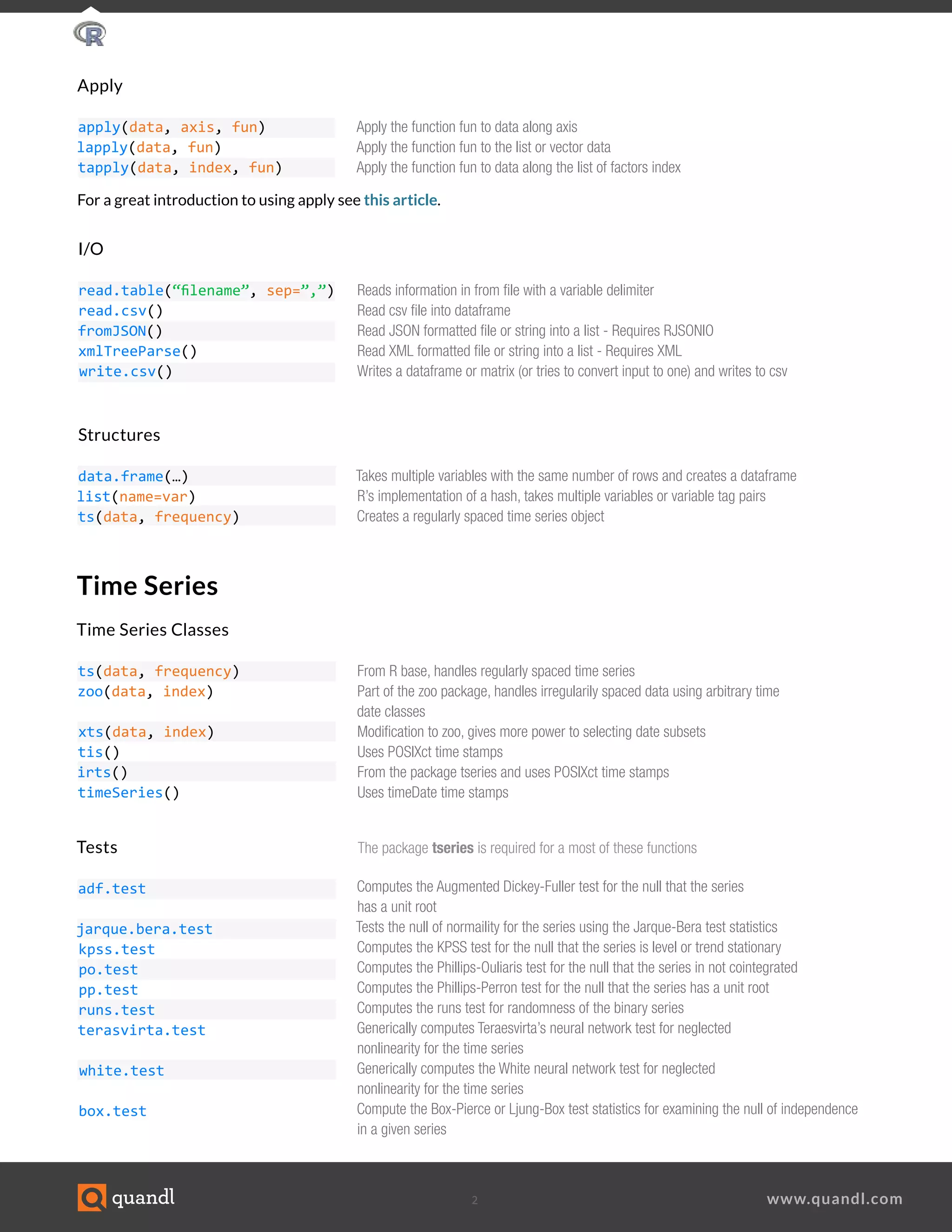
Plotting
plot(ts)
title(main, sub, xlab, ylab)
ggplot()
aes()
geom_line()
geom_boxplot()
xlab()
ylab()
ggtitle()
theme()
R base plot function
Adds labels to the currently open plot
Creates a ggplot object
Creates a properly formatted list of variables for use in ggplot
Plots data with a line connecting them
Plots data in the form of box and whiskers plot
Edit the x axis label
Edit the y axis label
Edit the plot title
Modify a large number of options for the plot from grid elements to colors
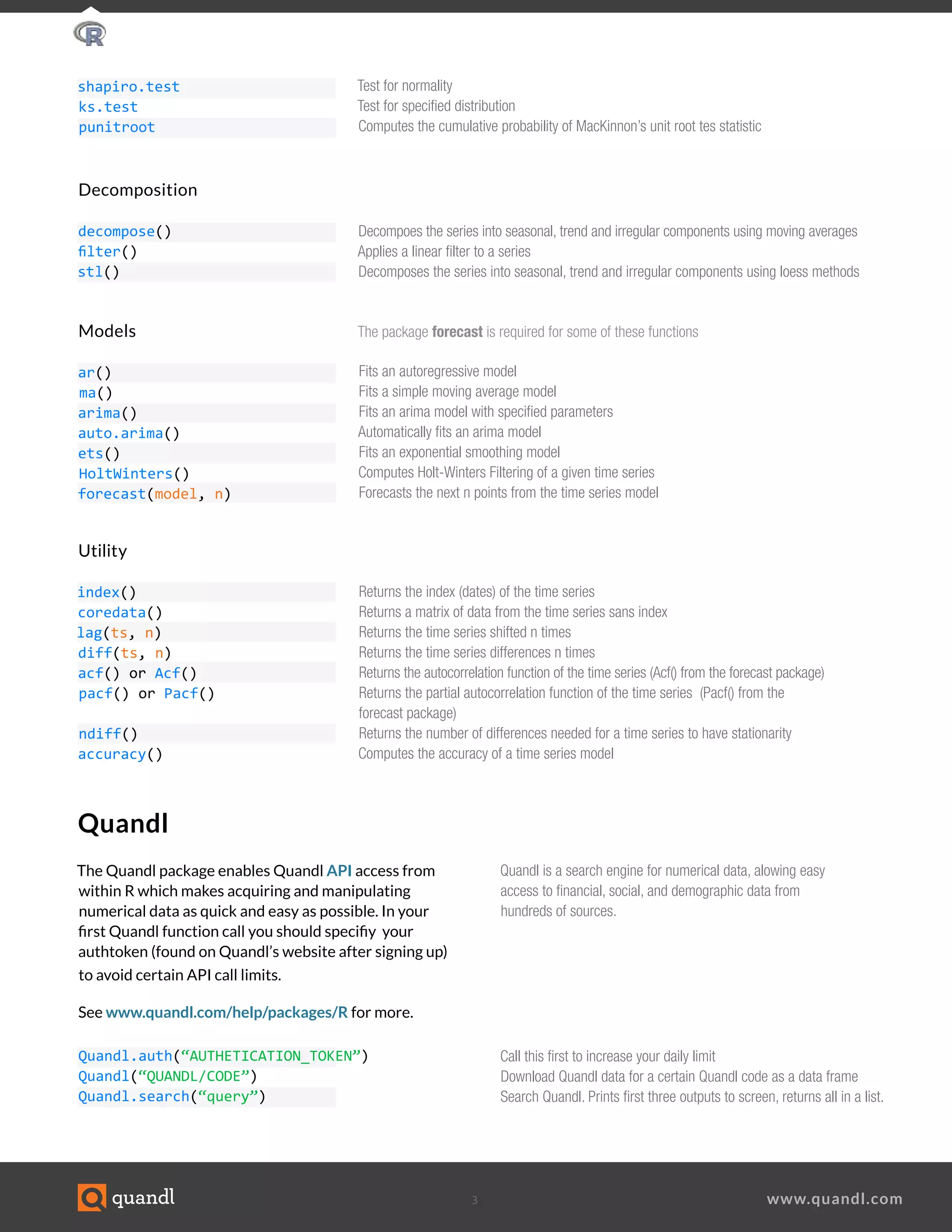
Aside from the built in plotting function in R, ggplot2 is a very powerful plotting package.
See http://docs.ggplot2.org/current/ for complete documentation.
Plotting example with ggplot2
library(Quandl)
library(ggplot2)
data_series <- Quandl(“GOOG/NASDAQ_AAPL”, start_date=”2005-01-01”)[,c(1,5)]
my.plot <- ggplot(data=data_series, aes(x=Date, y=Close)) +
geom_line(color=”#FAB521”) + # Adding a colored line
theme(panel.background = element_rect(fill=’#393939’), panel.grid.major.x = element_blank(),
panel.grid.major.y = element_line(colour=’white’, size=0.1),
panel.grid.minor = element_line(colour=’white’, size=0.1)) + # modifying background color
# and grid options
xlab(“Date”) + ylab(“Closing Price”) + ggtitle(“AAPL”) # Adding titles
my.plot # Generates the plot