Downloaded 114 times


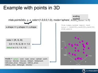
![Mayavi “API” or scripting with mlab # Create the data. from numpy import pi, sin, cos, mgrid dphi, dtheta = pi/250.0, pi/250.0 [phi,theta] = mgrid[0:pi+dphi*1.5:dphi,0:2*pi+dtheta*1.5:dtheta] m0 = 4; m1 = 3; m2 = 2; m3 = 3; m4 = 6; m5 = 2; m6 = 6; m7 = 4; r = sin(m0*phi)**m1 + cos(m2*phi)**m3 + sin(m4*theta)**m5 + cos(m6*theta)**m7 x = r*sin(phi)*cos(theta) y = r*cos(phi) z = r*sin(phi)*sin(theta) # View it. from enthought.mayavi import mlab s = mlab.mesh(x, y, z) mlab.show()](https://image.slidesharecdn.com/scpmayavi-2010-03-19-100319161651-phpapp01/85/Scientific-Computing-with-Python-Webinar-March-19-3D-Visualization-with-Mayavi-8-320.jpg)


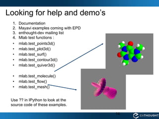
![Mlab and Traits (mlab_traits_ui.py) class ActorViewer(HasTraits): scene = Instance(MlabSceneModel, ()) view = View(Item(name='scene‘, editor=SceneEditor(scene_class=MayaviScene), show_label=False, resizable=True, height=500, width=500), resizable=True) def __init__(self, **traits): HasTraits.__init__(self, **traits) self.generate_data() def generate_data(self): X, Y = mgrid[-2:2:100j, -2:2:100j] R = 10*sqrt(X**2 + Y**2) Z = sin(R)/R self.scene.mlab.surf(X, Y, Z, colormap='gist_earth') if __name__ == '__main__': a = ActorViewer() a.configure_traits()](https://image.slidesharecdn.com/scpmayavi-2010-03-19-100319161651-phpapp01/85/Scientific-Computing-with-Python-Webinar-March-19-3D-Visualization-with-Mayavi-15-320.jpg)


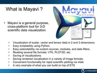
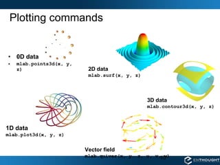
Mayavi is a cross-platform tool designed for 3D scientific data visualization, supporting scalar, vector, and tensor data in multiple dimensions. It offers features like Python scripting, custom modules, and the ability to read and save various file formats. The document provides example code snippets for using Mayavi's mlab interface to generate and display 3D visualizations.