Download as PDF, PPTX
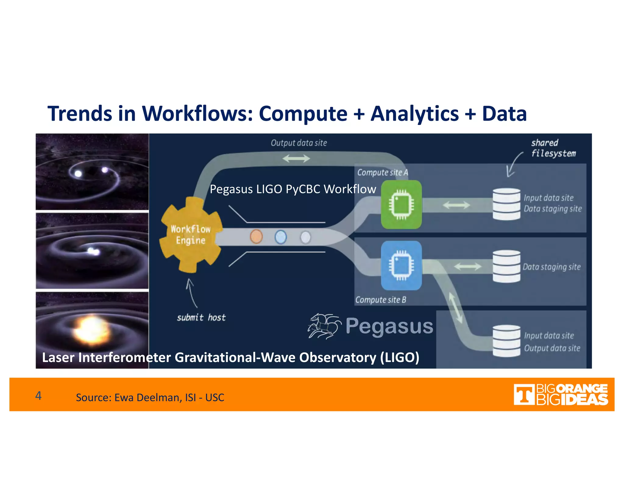
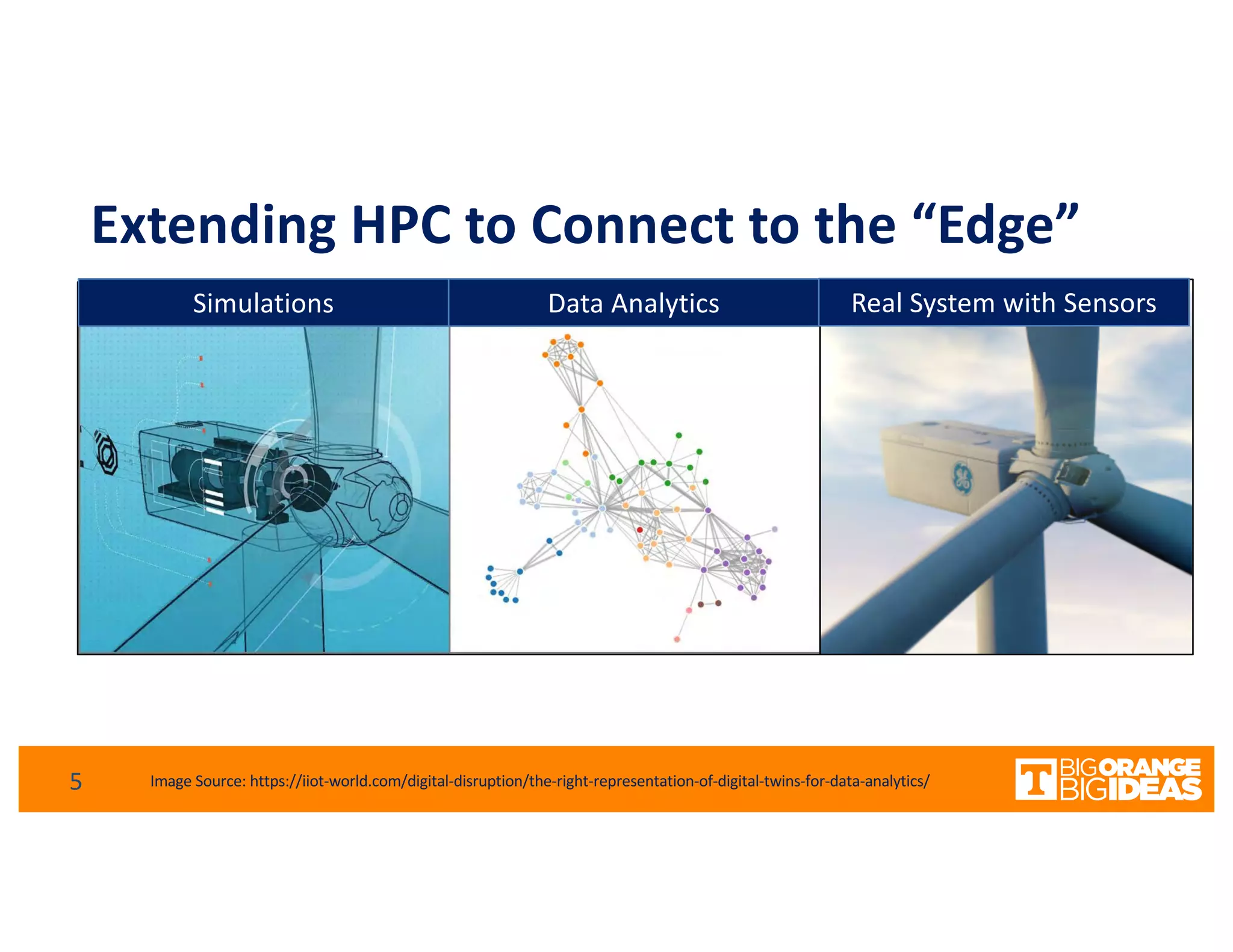
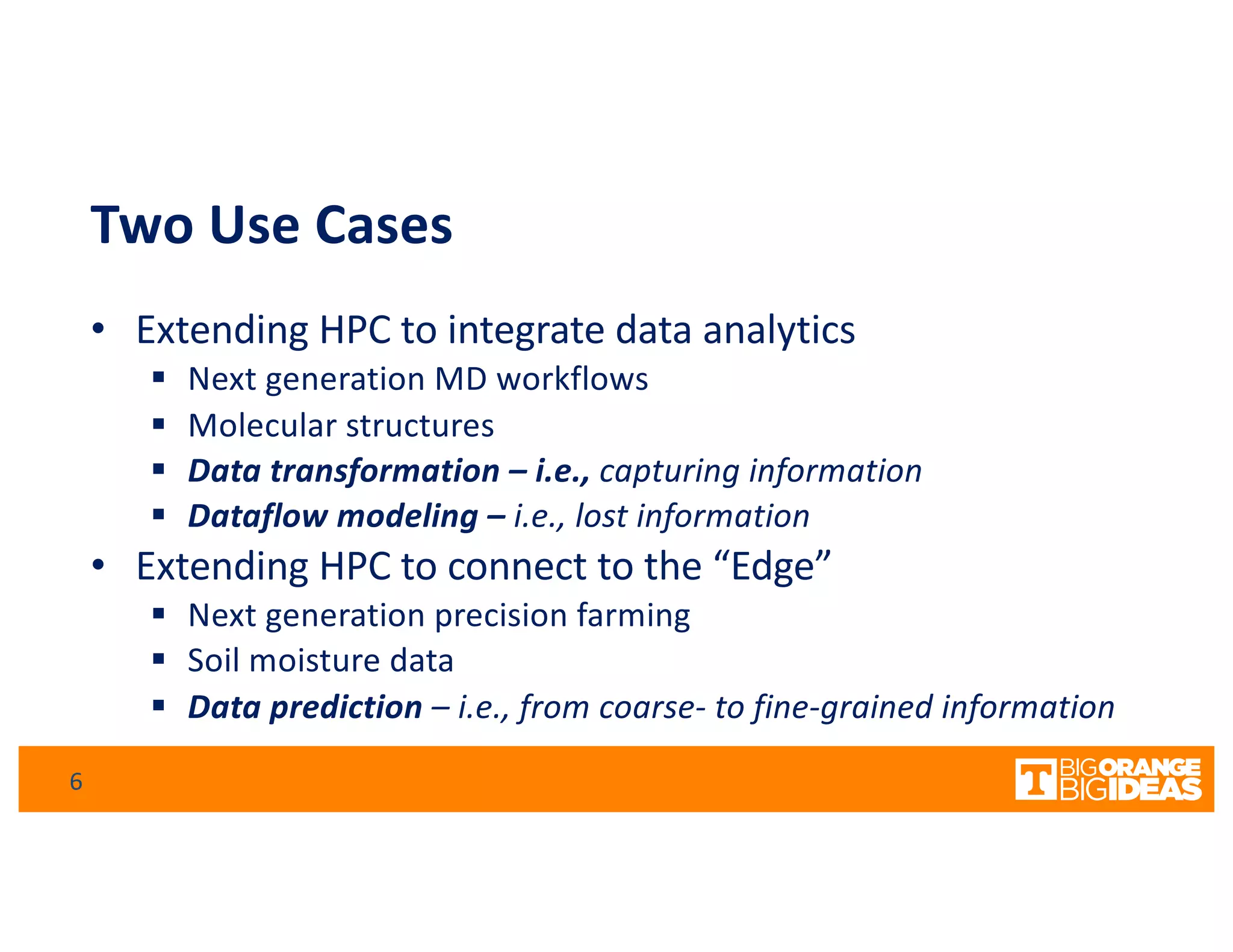
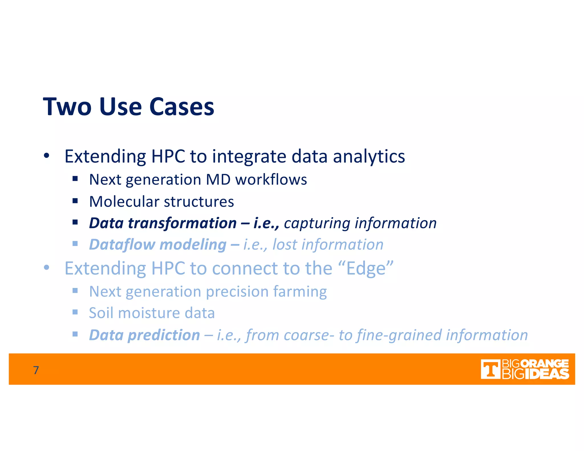
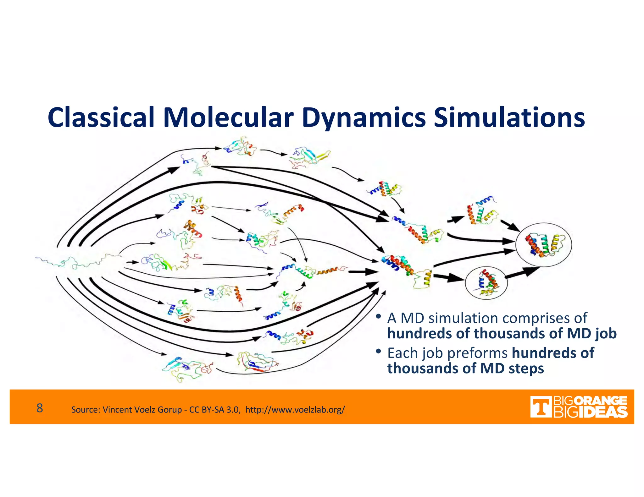
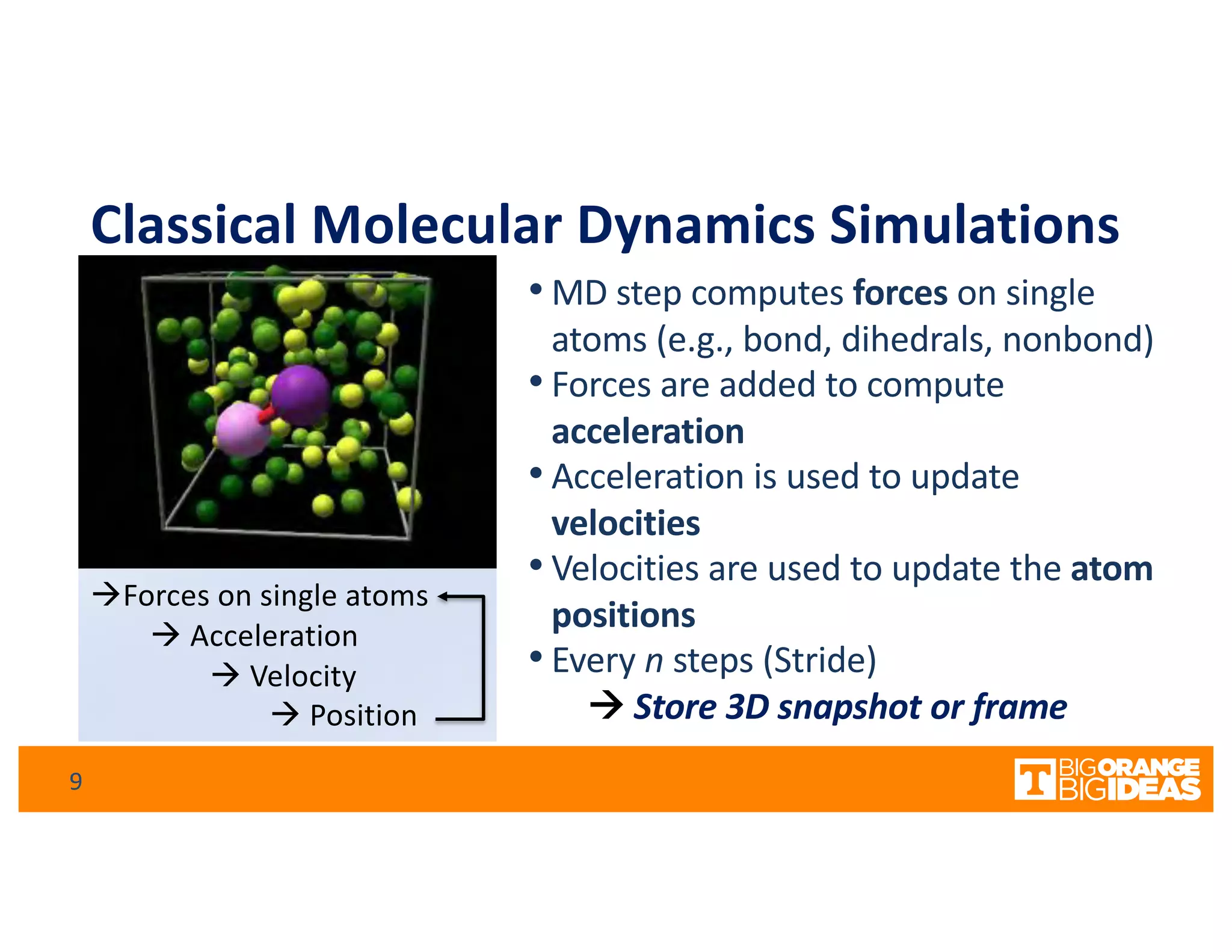
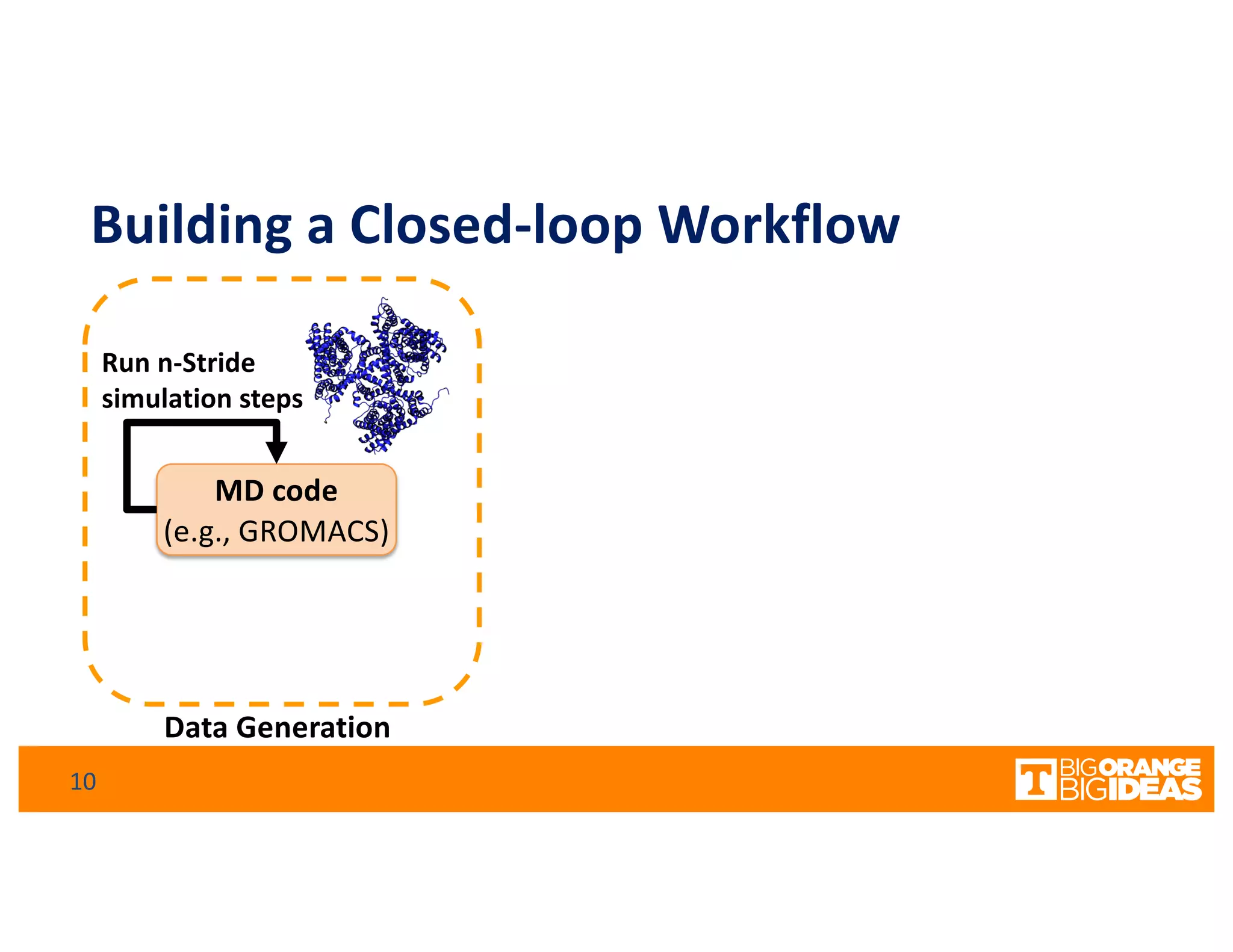
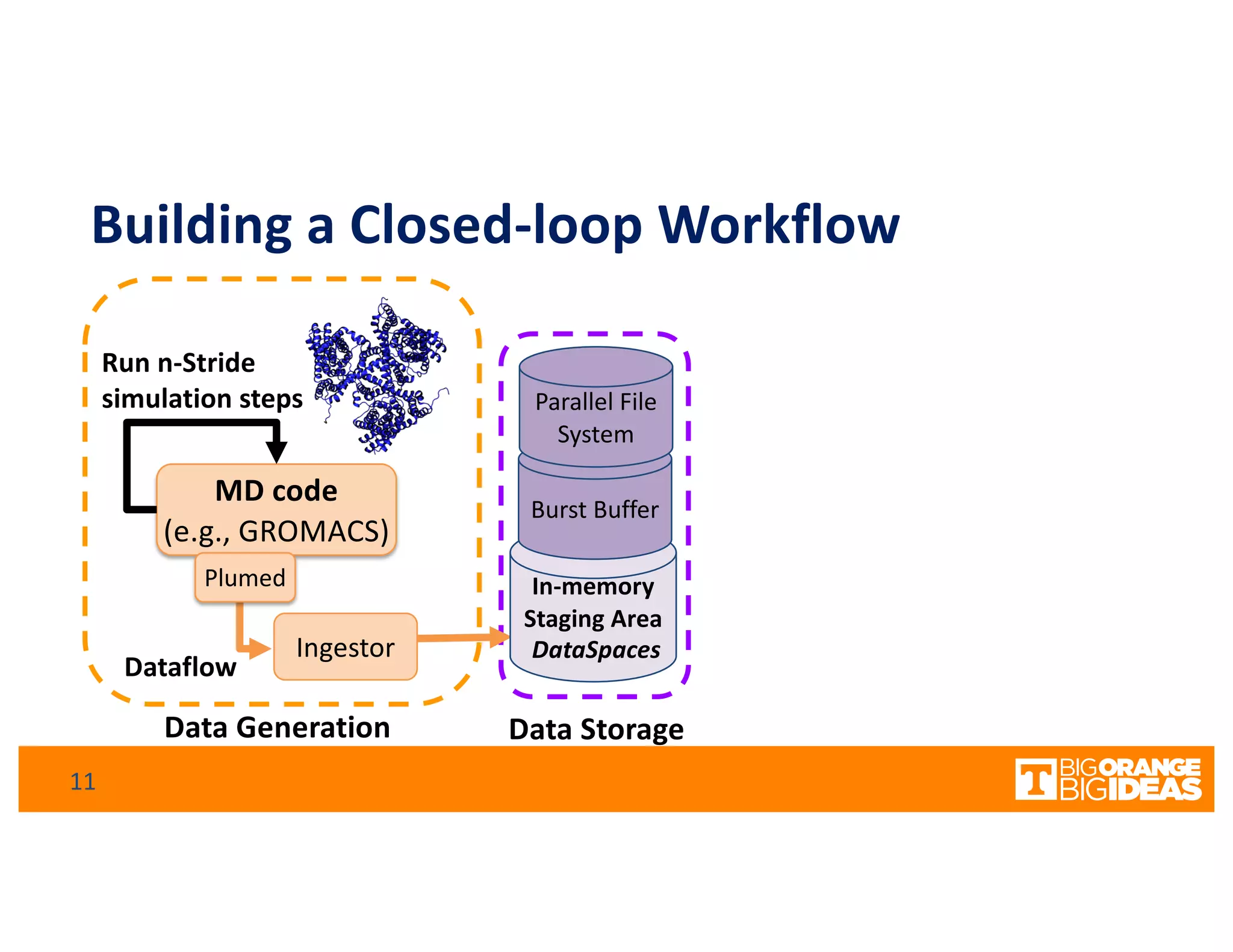
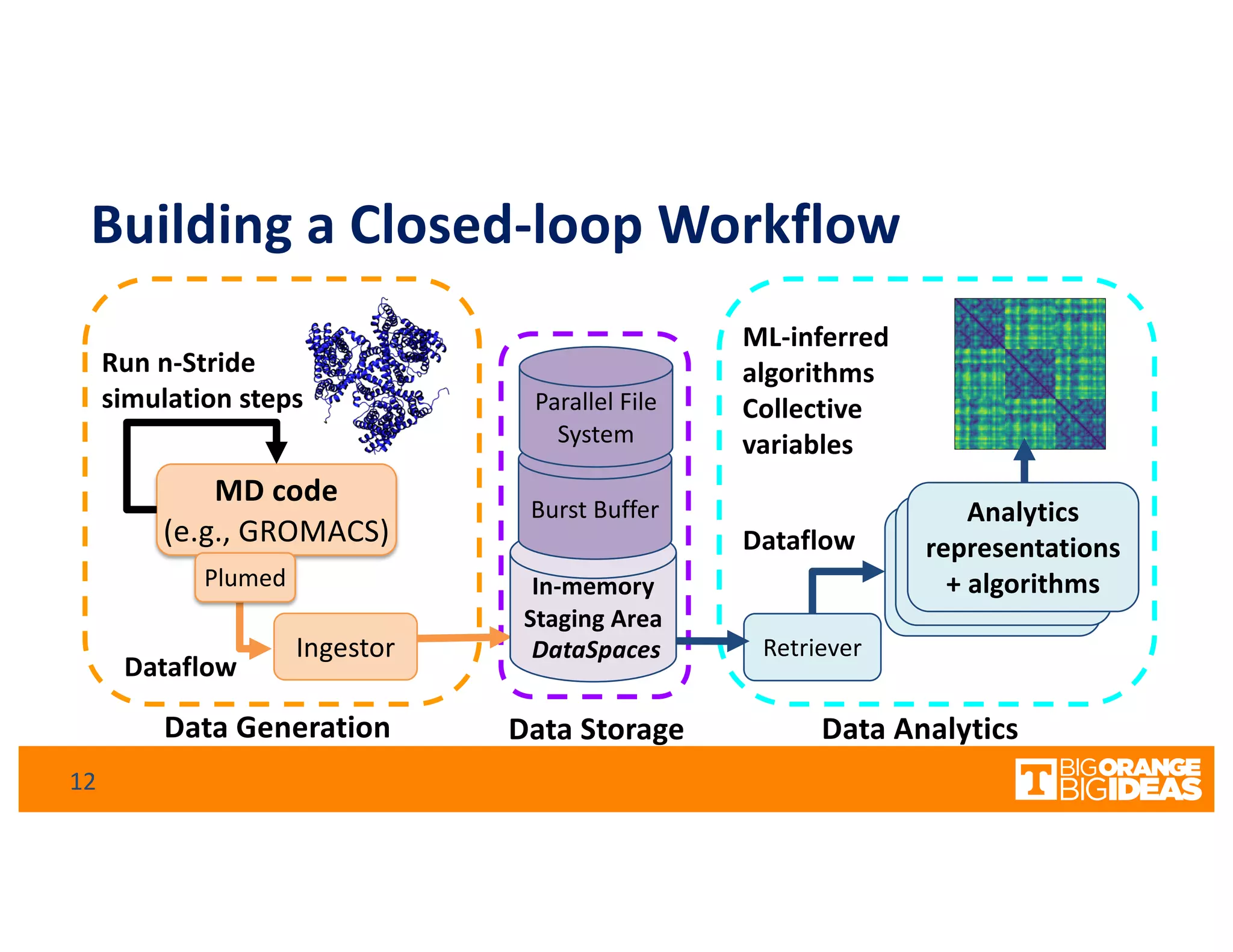
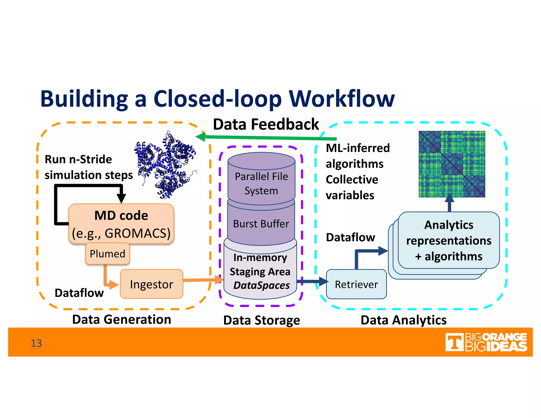
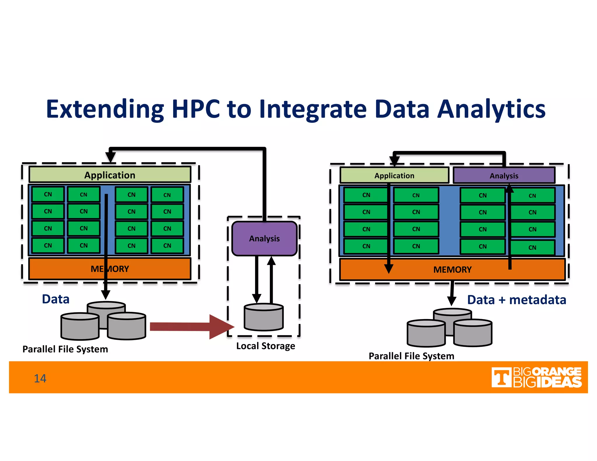
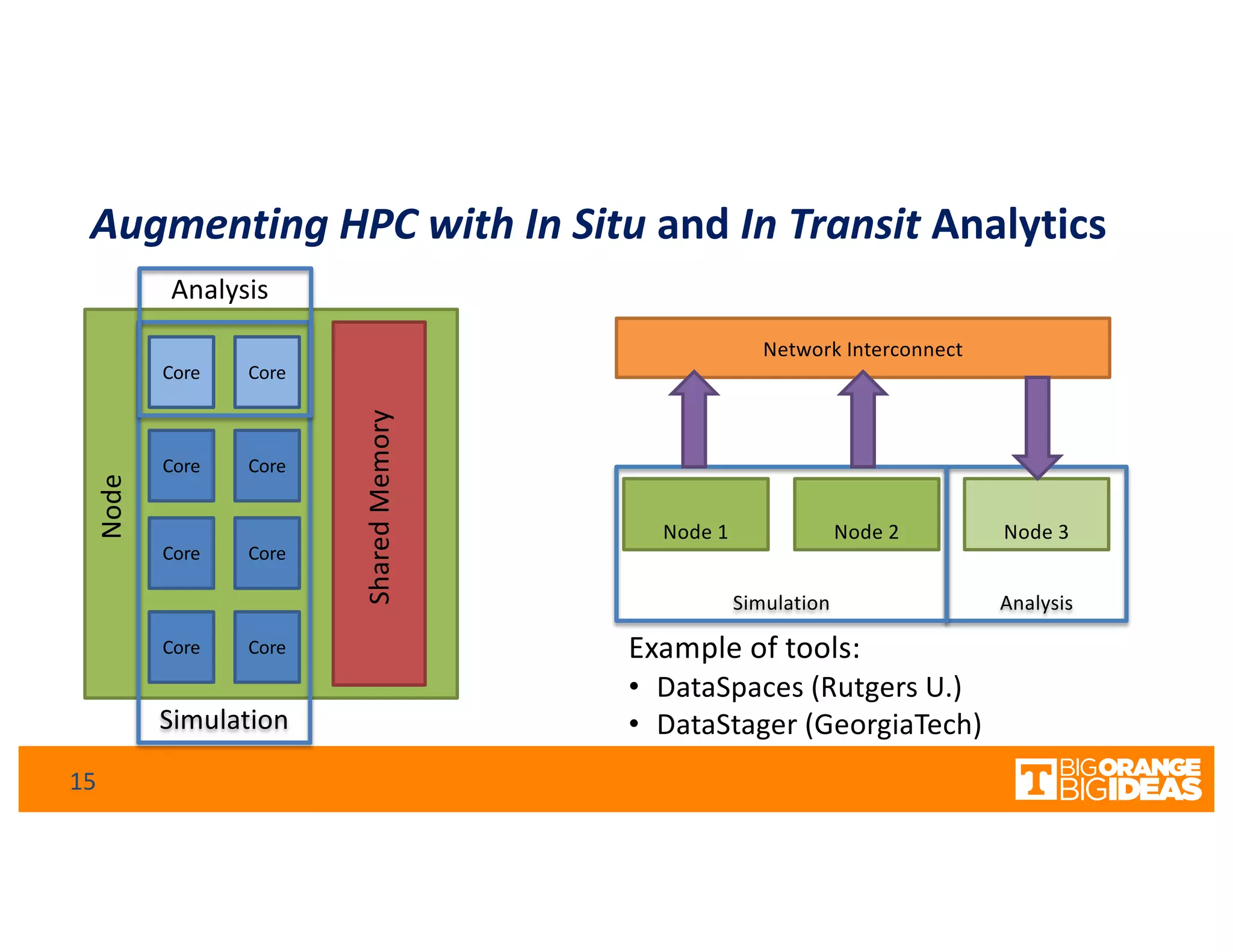
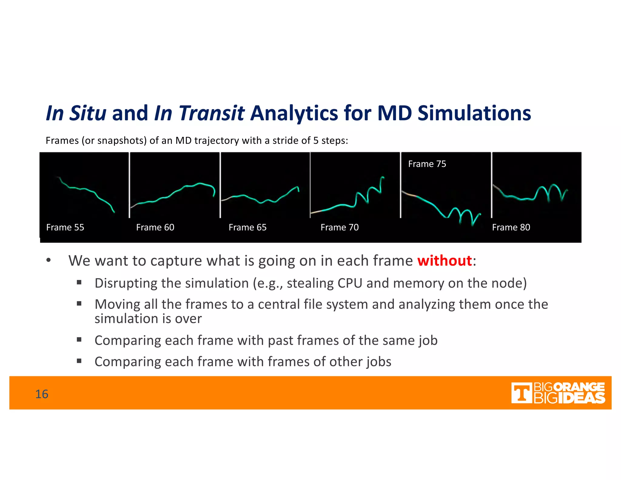

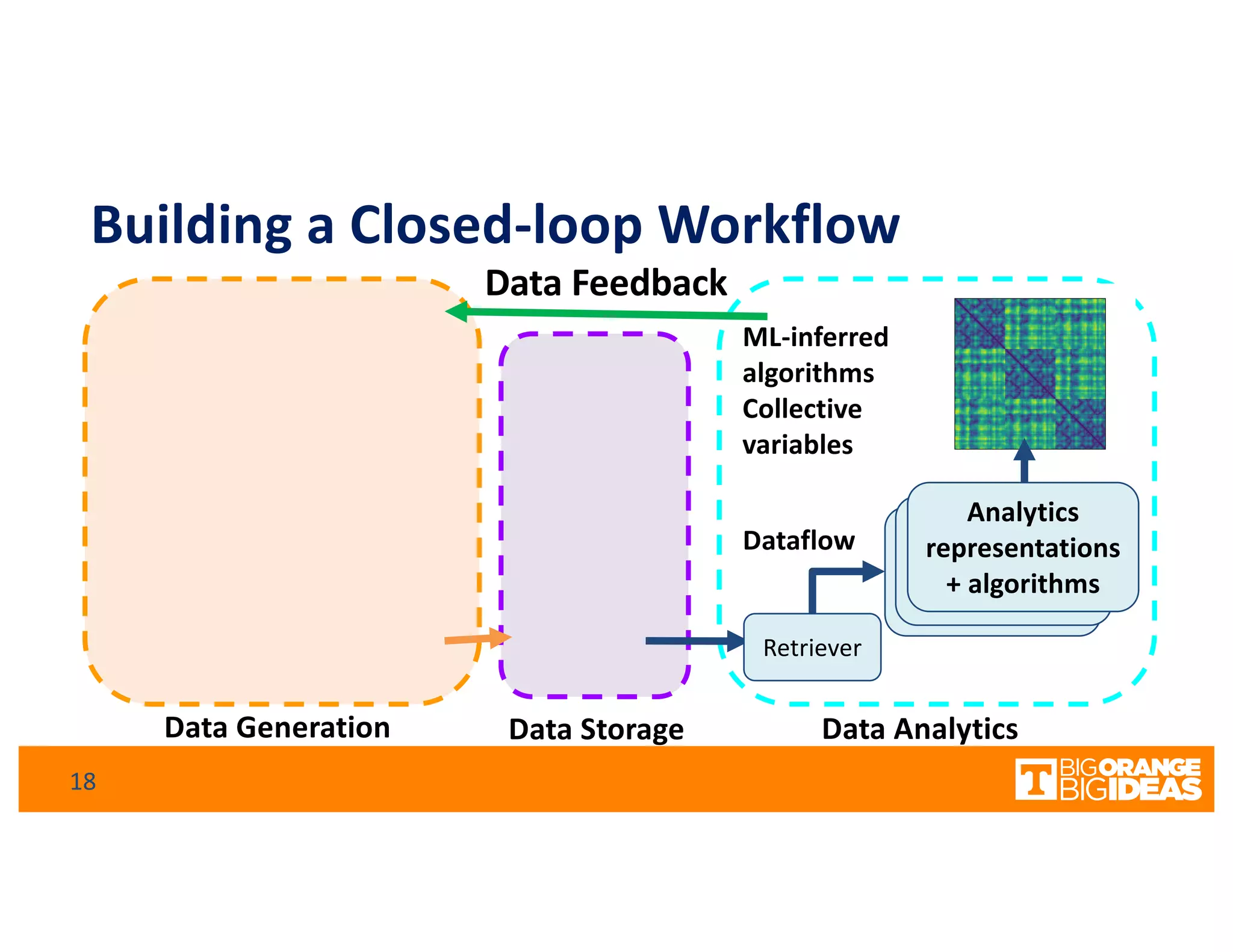
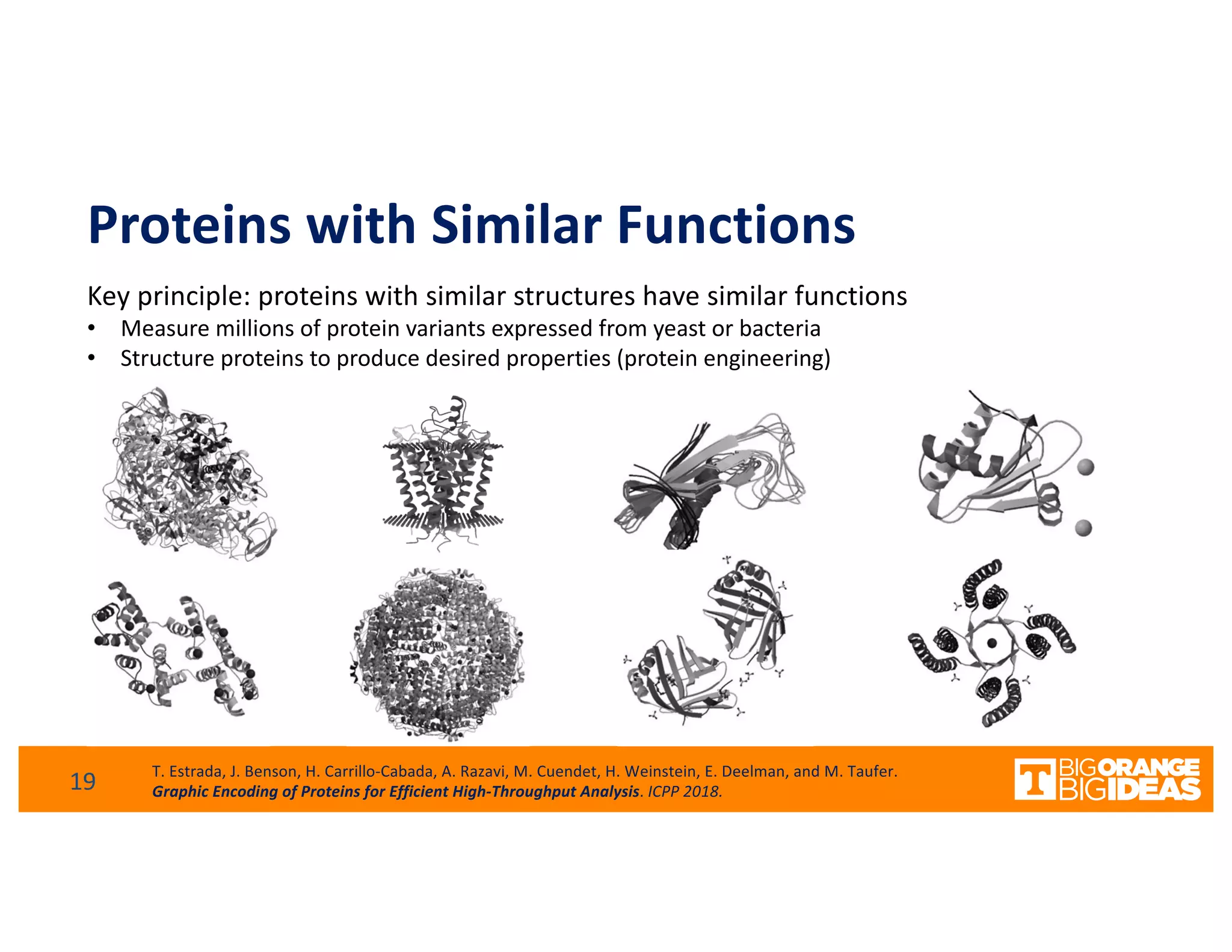
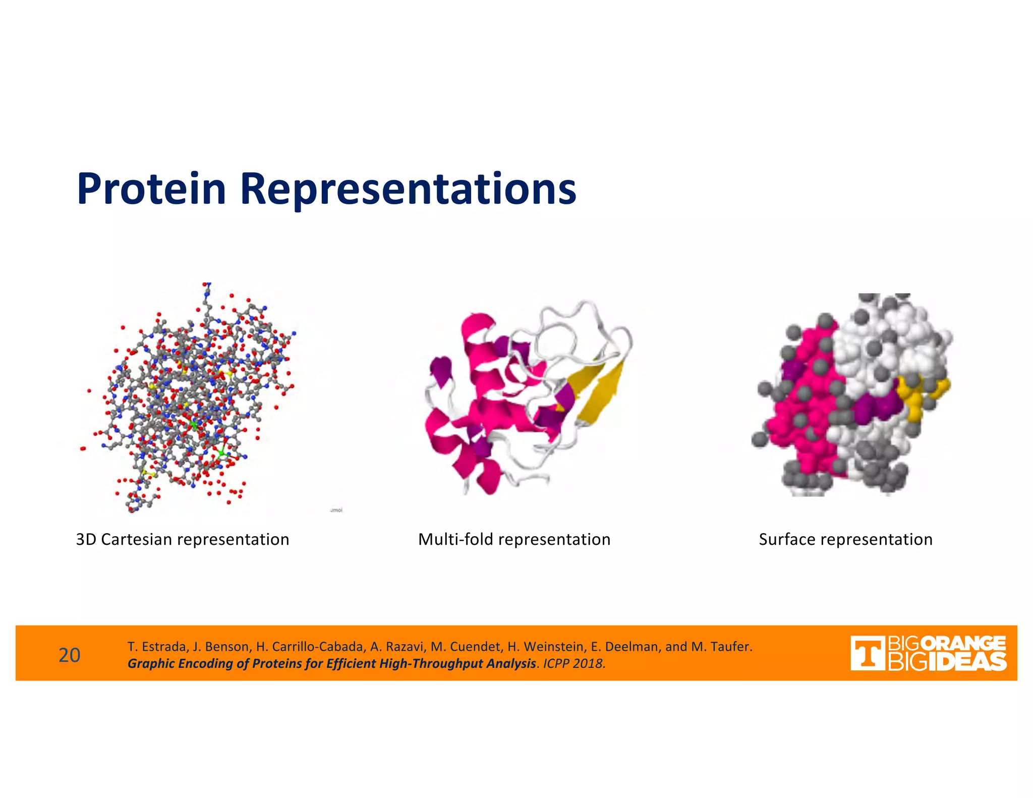
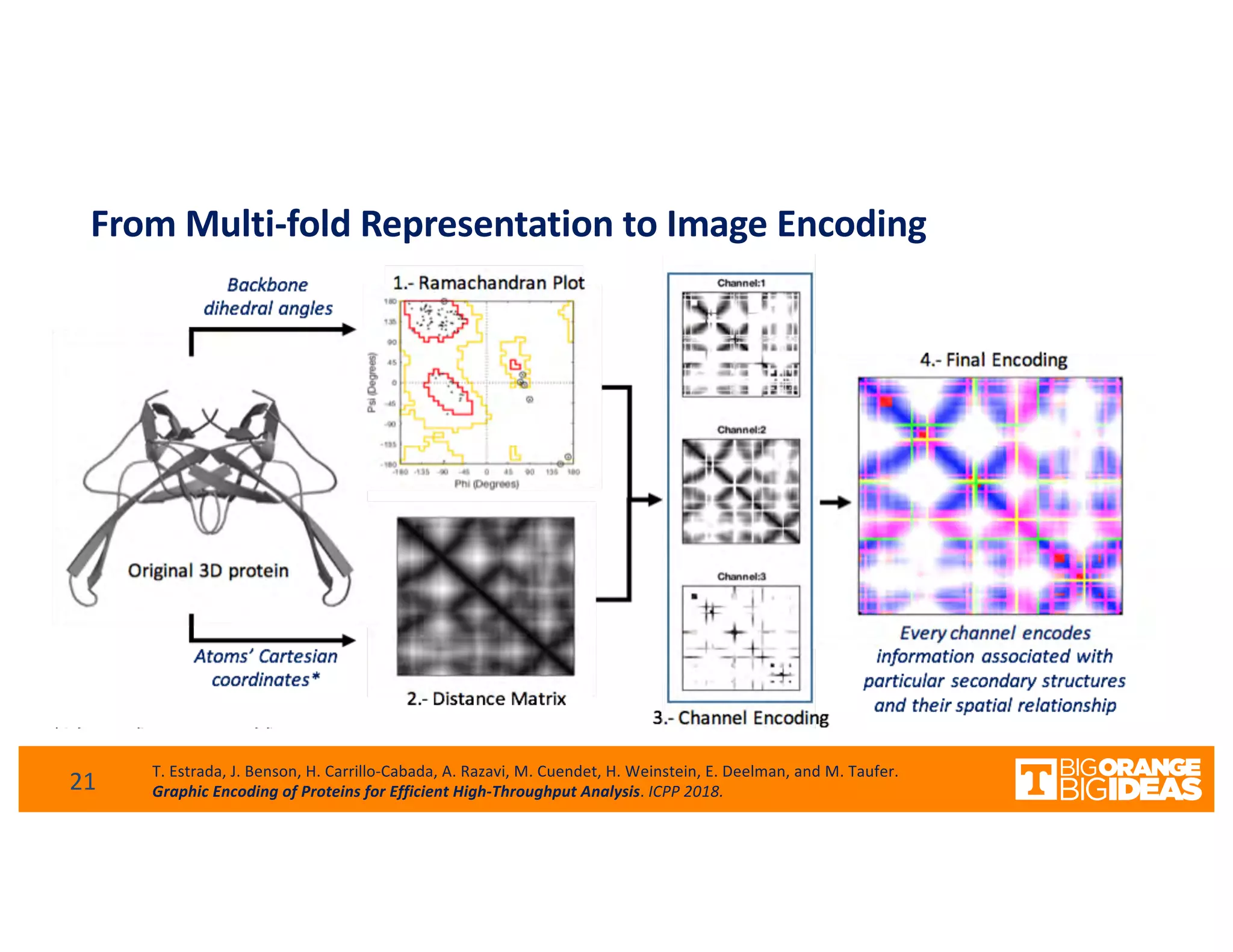
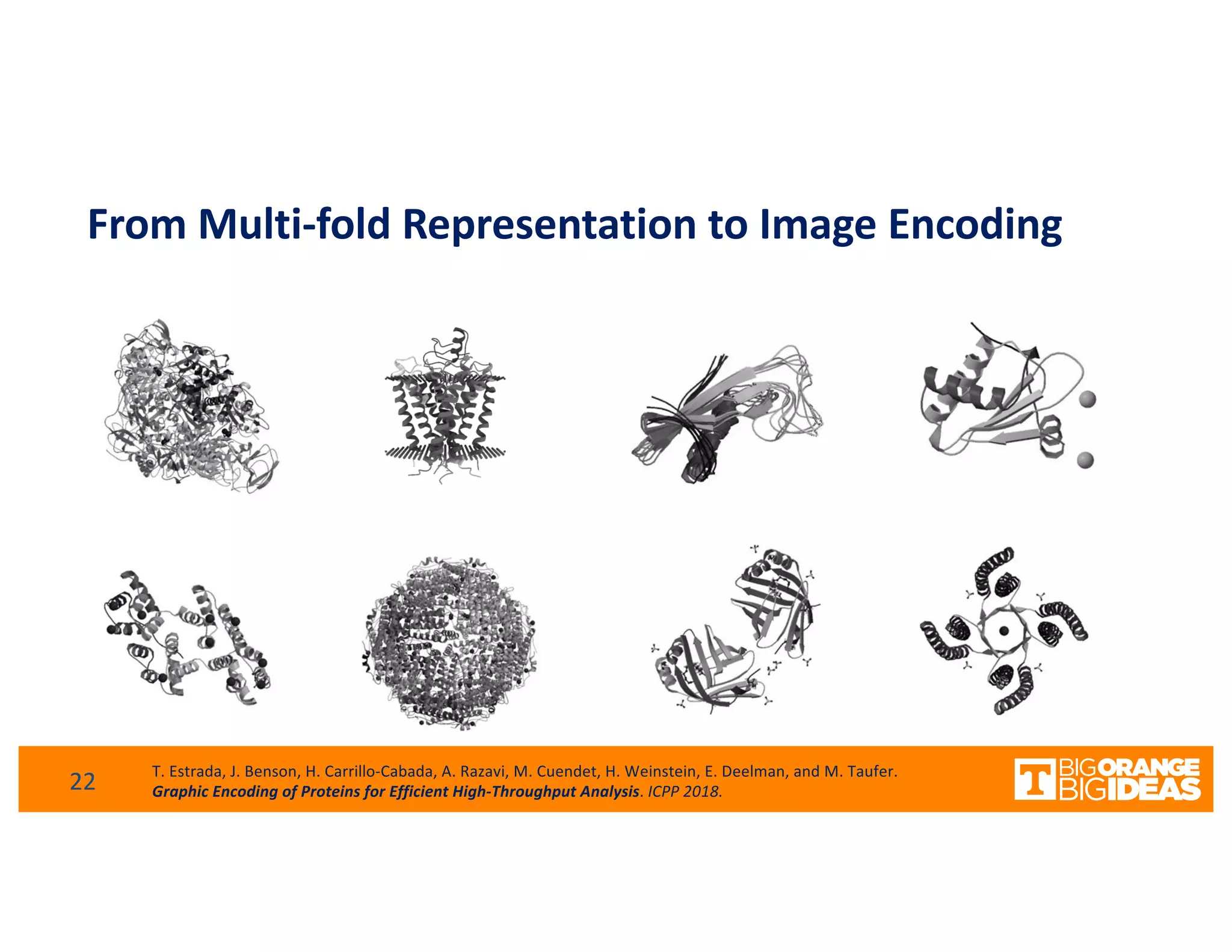
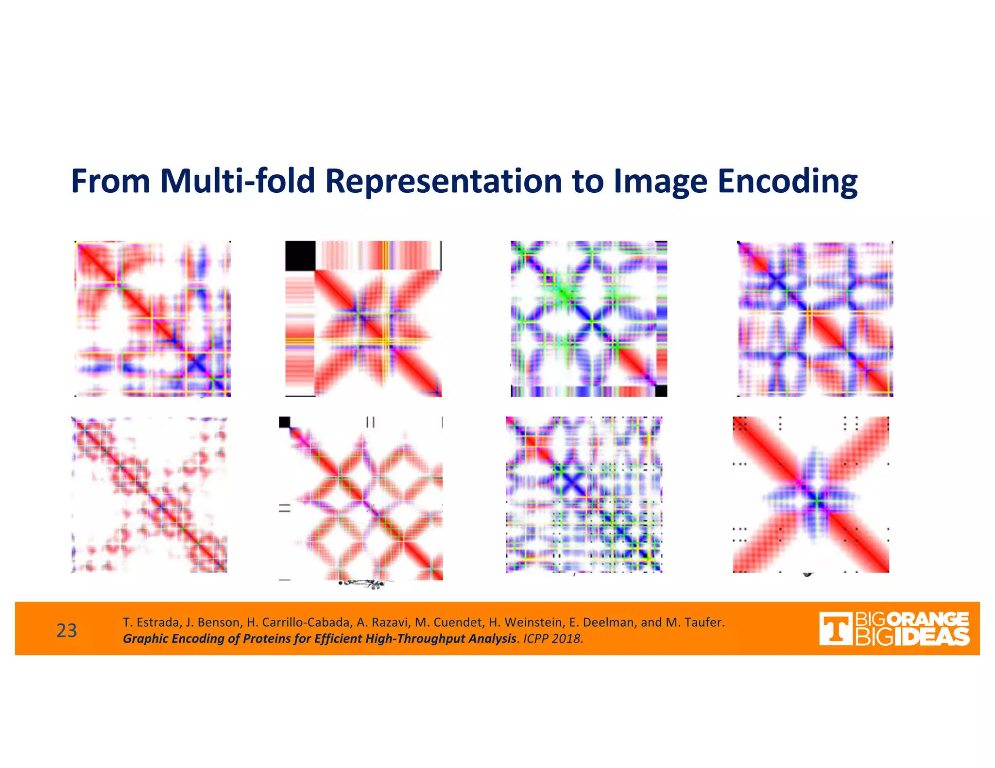
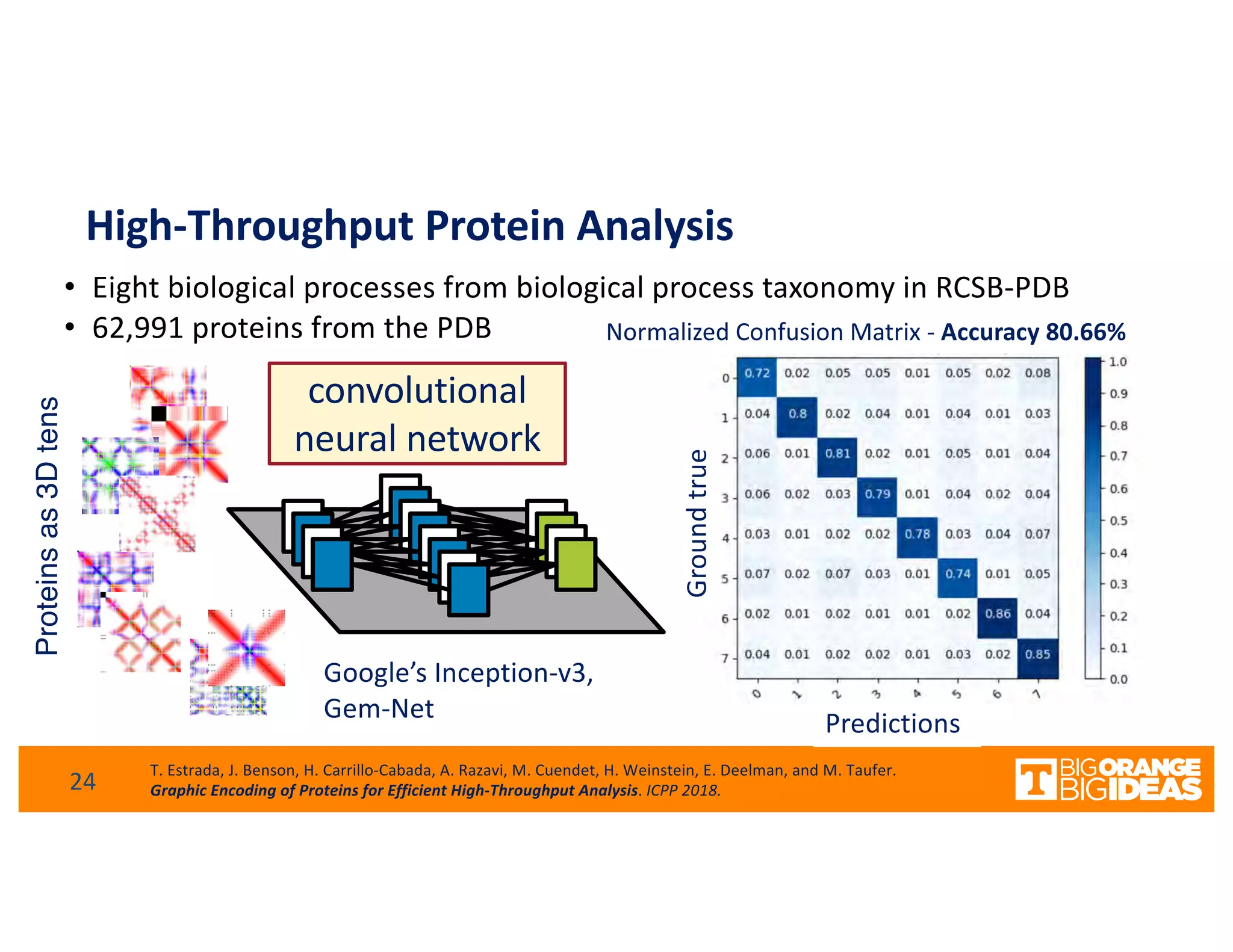
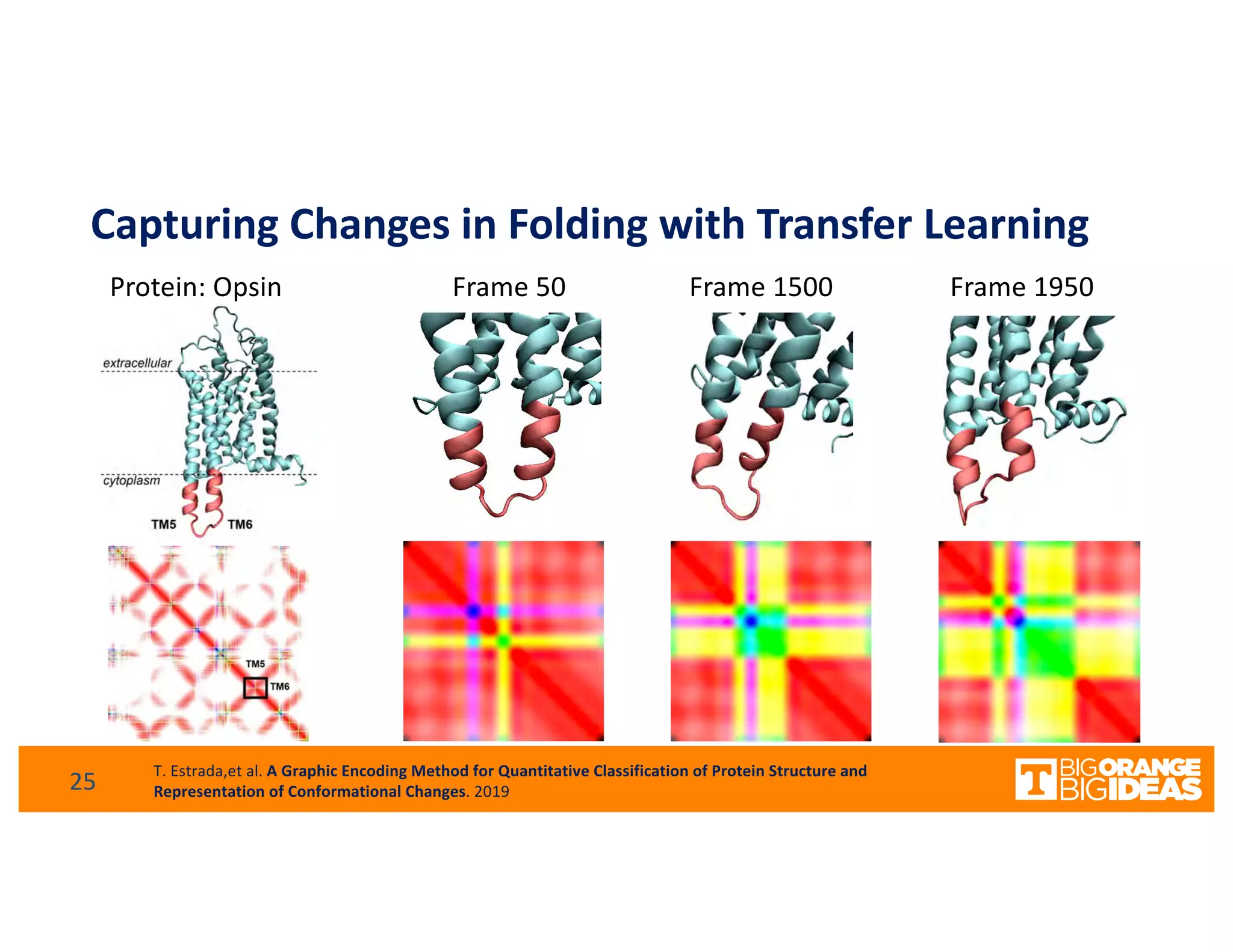
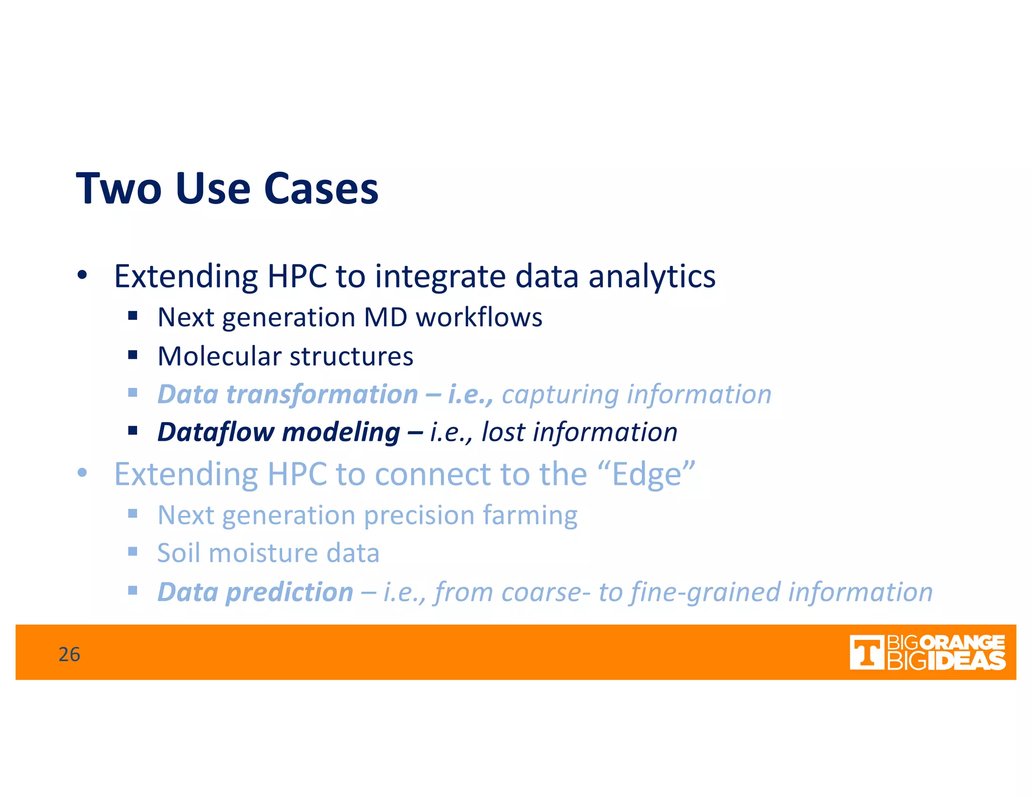

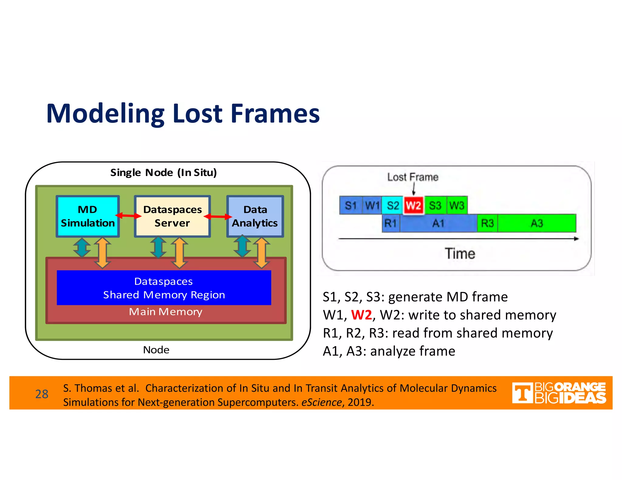
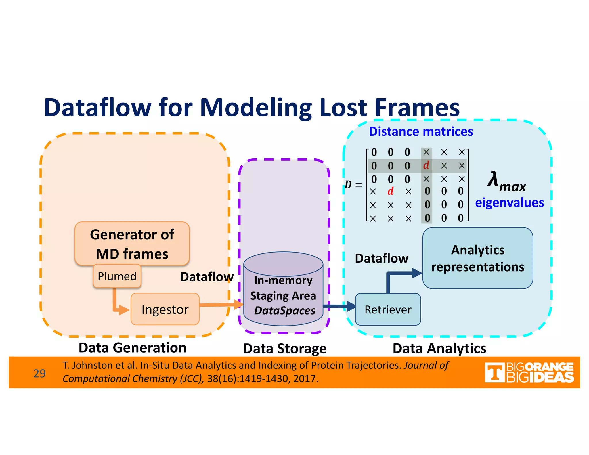
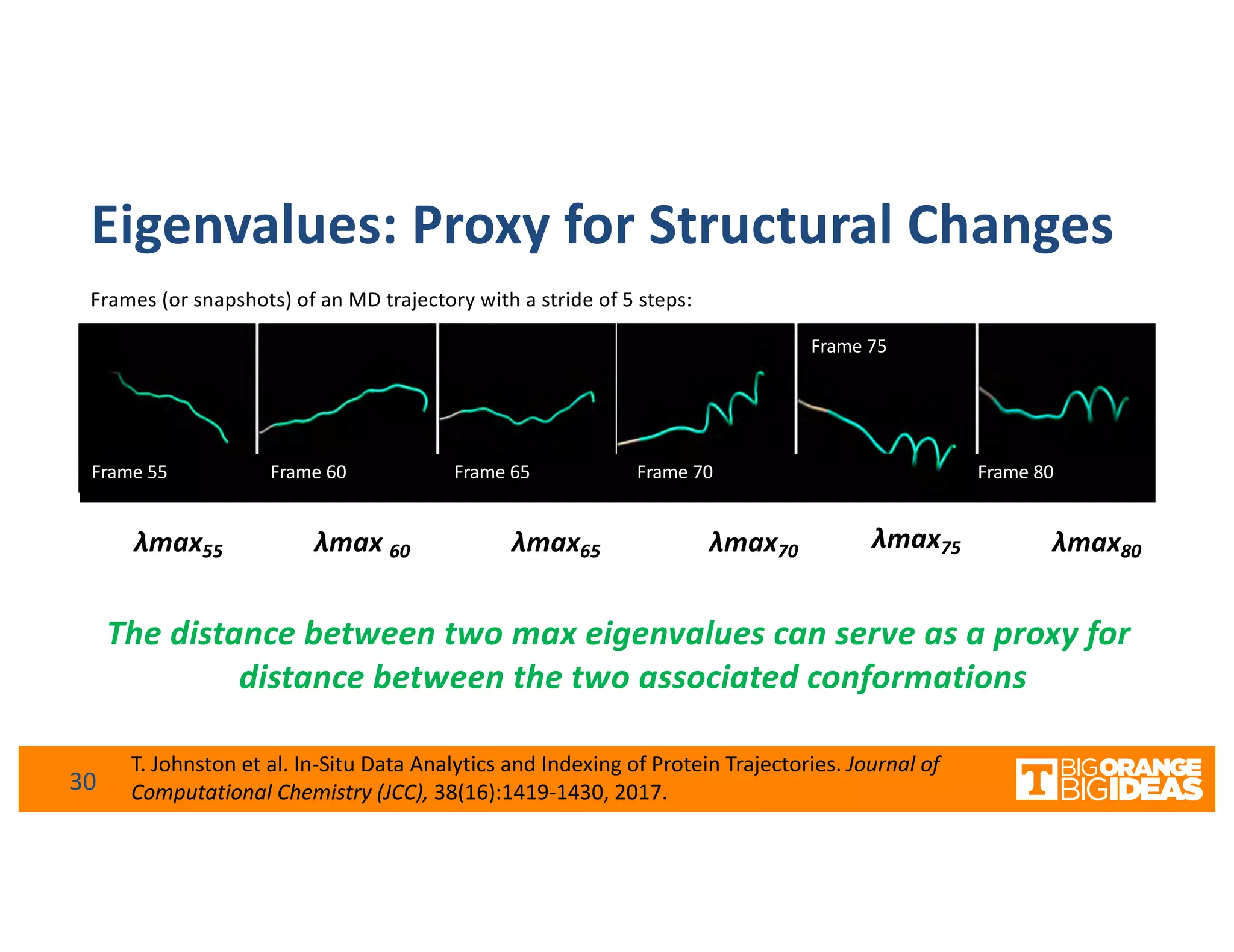
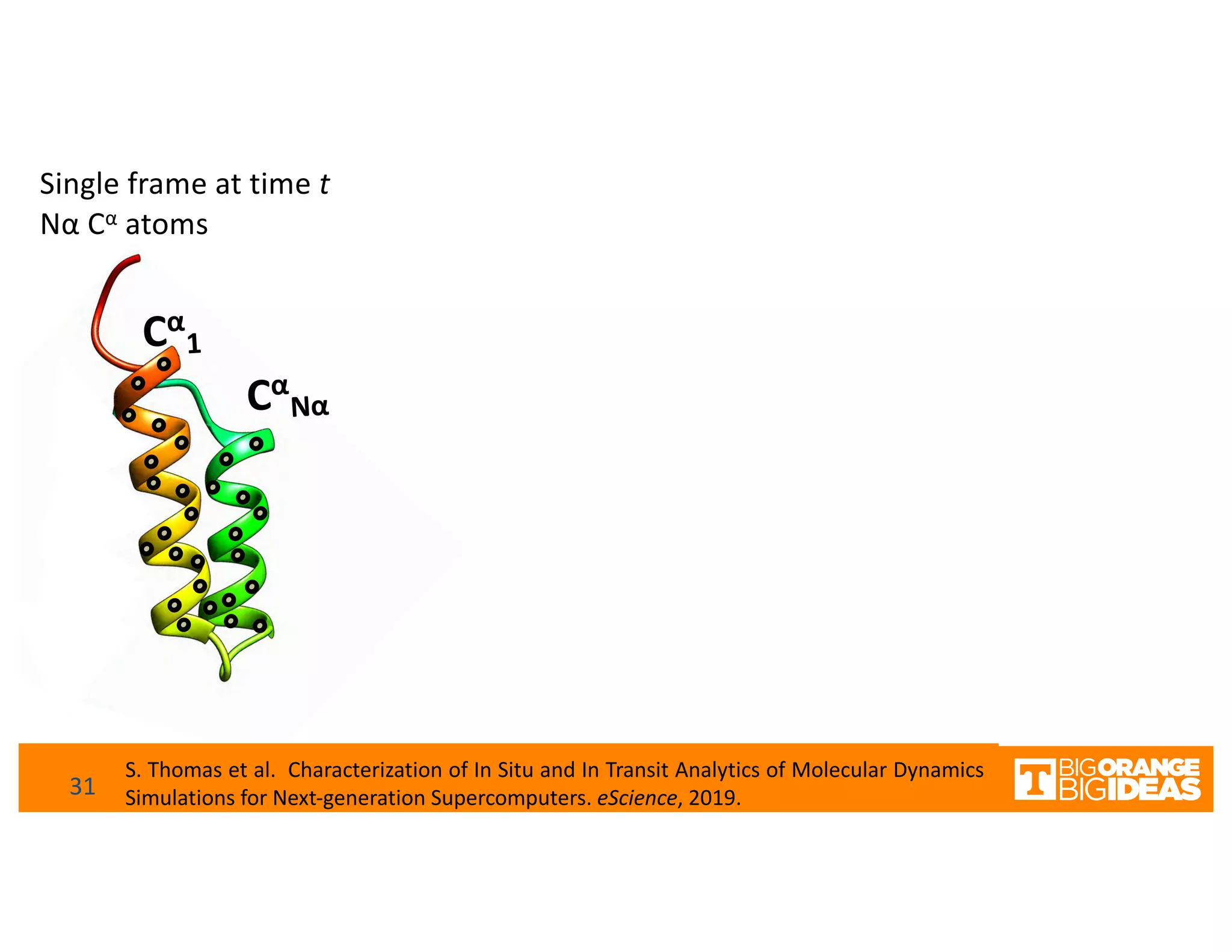
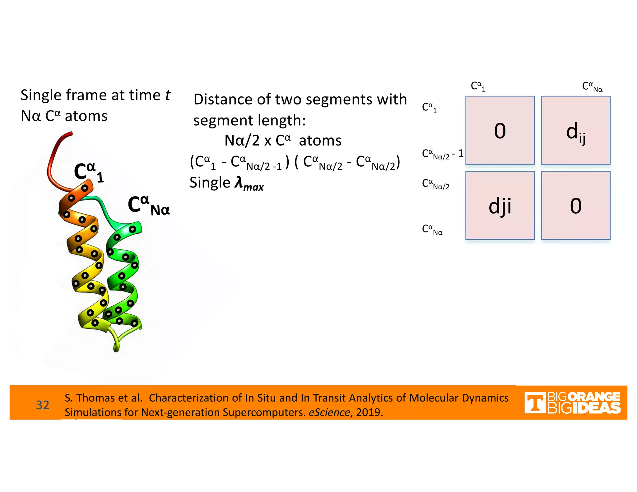
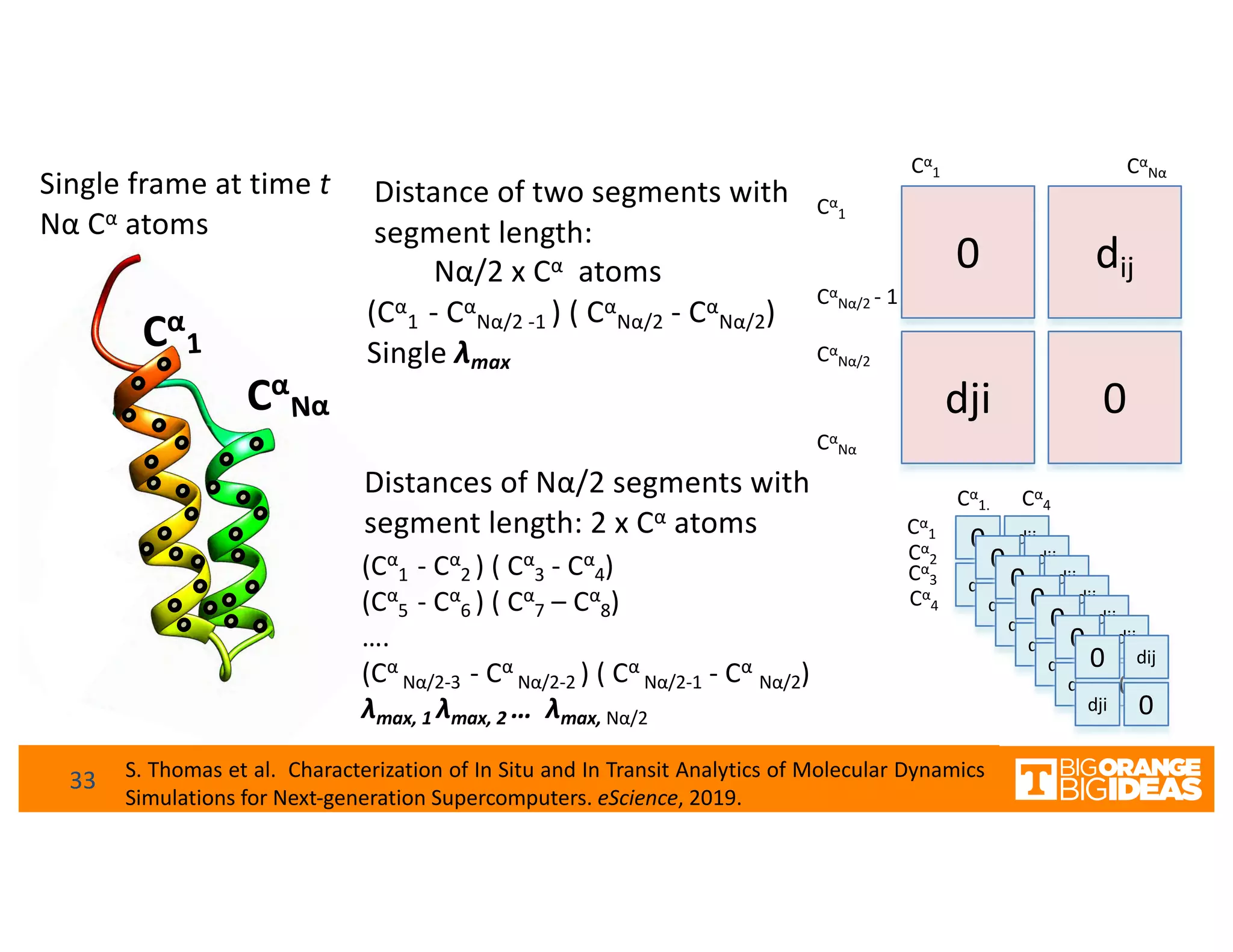
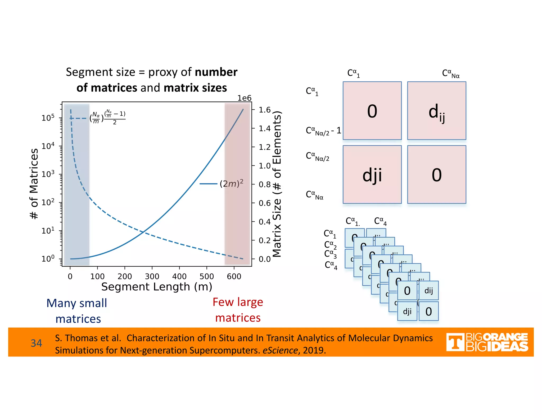
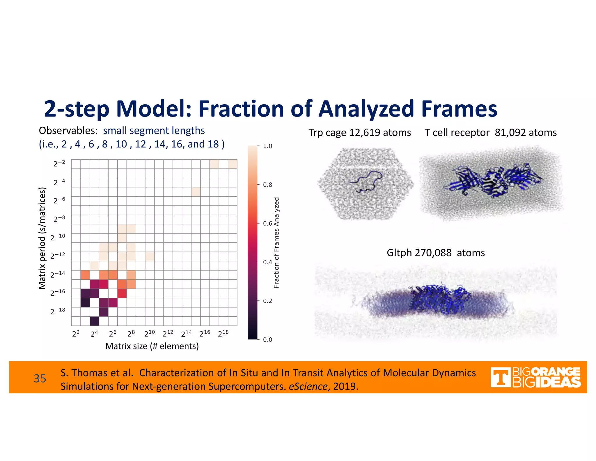
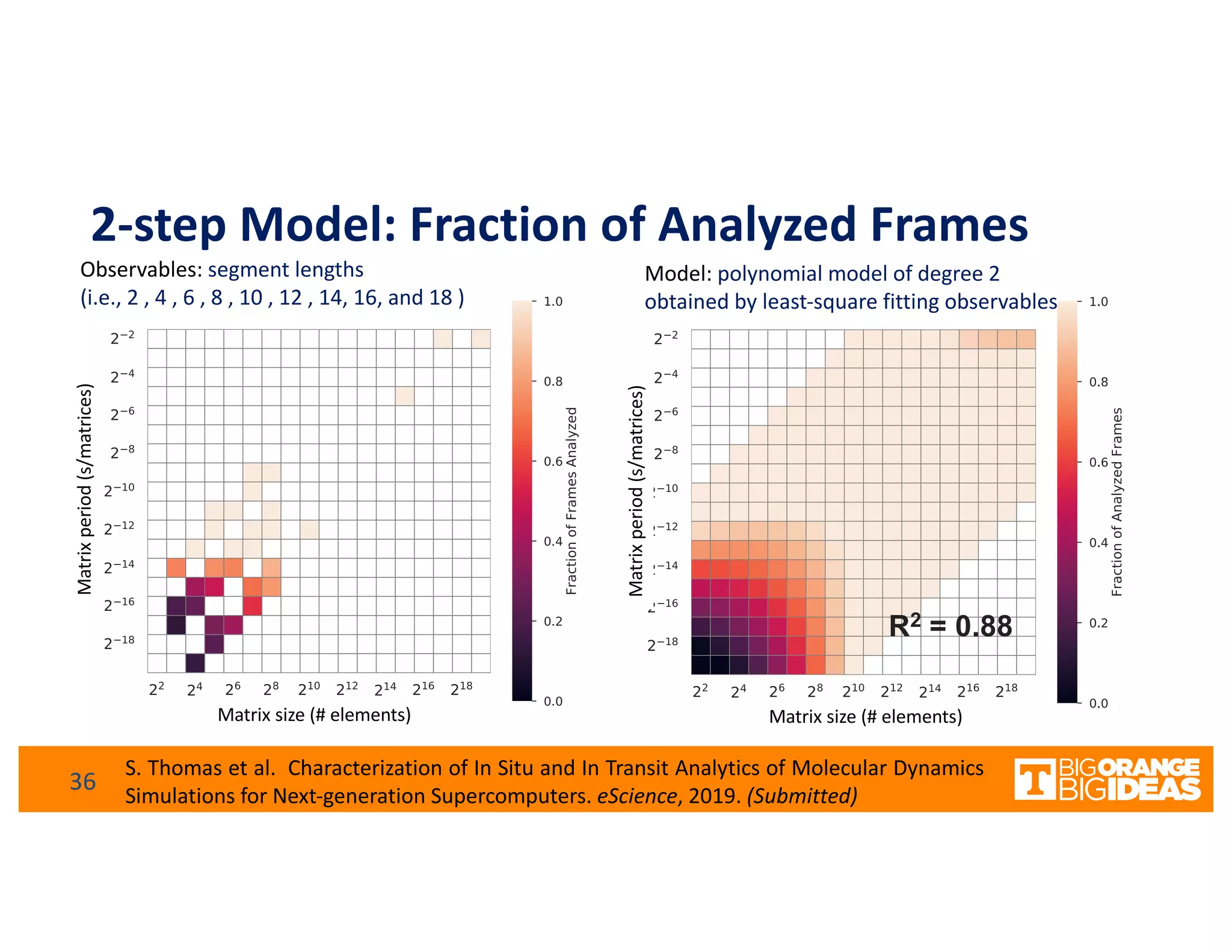
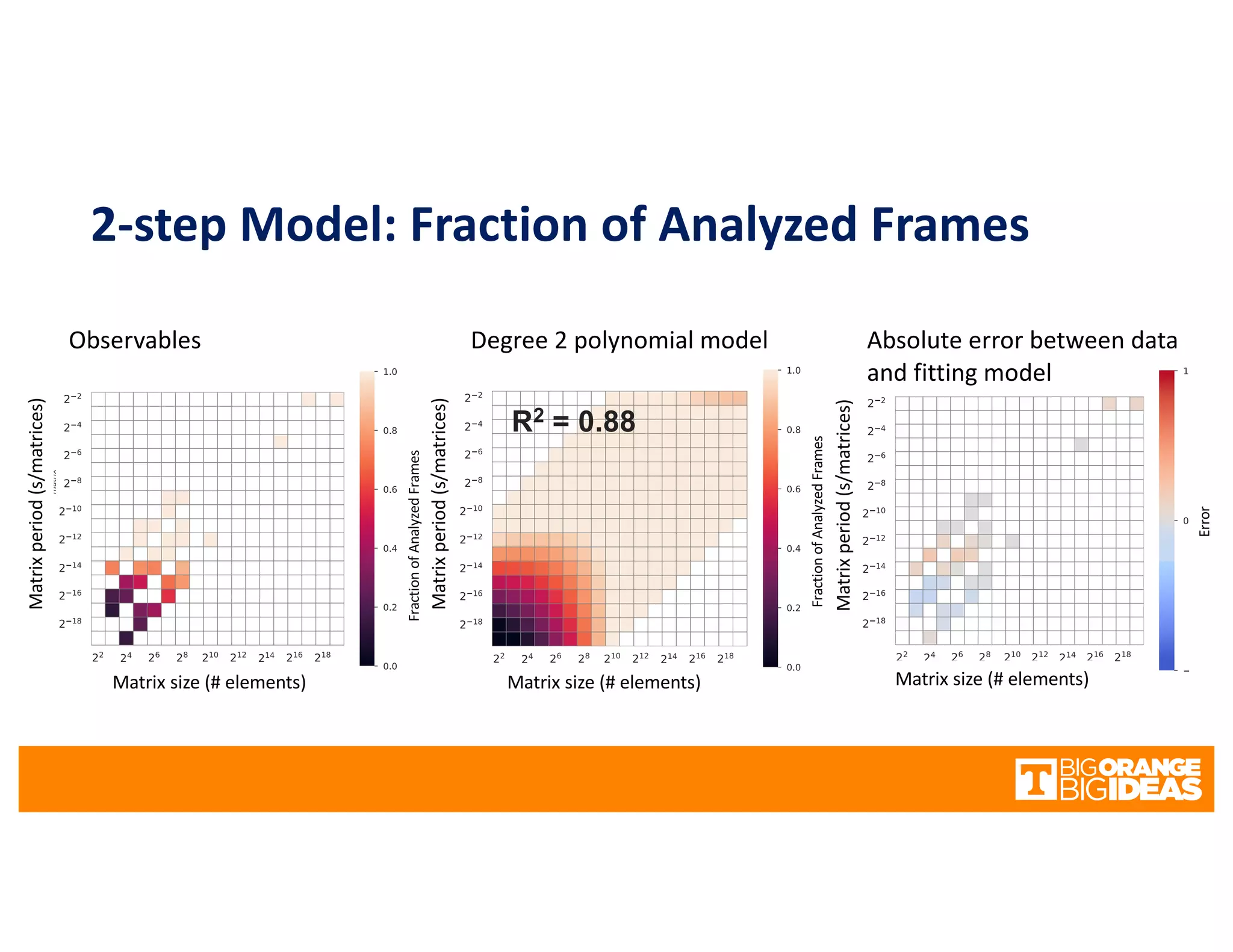
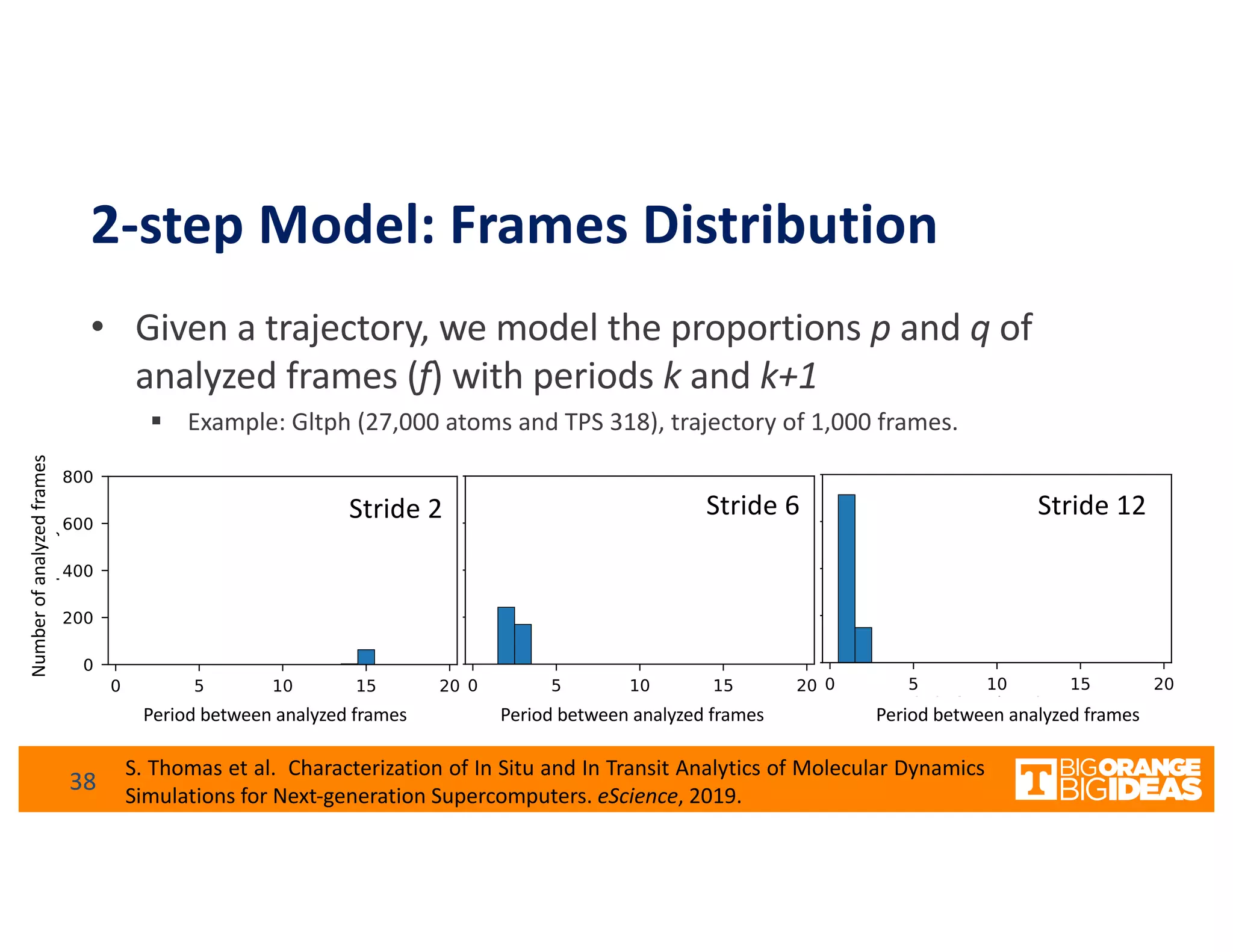
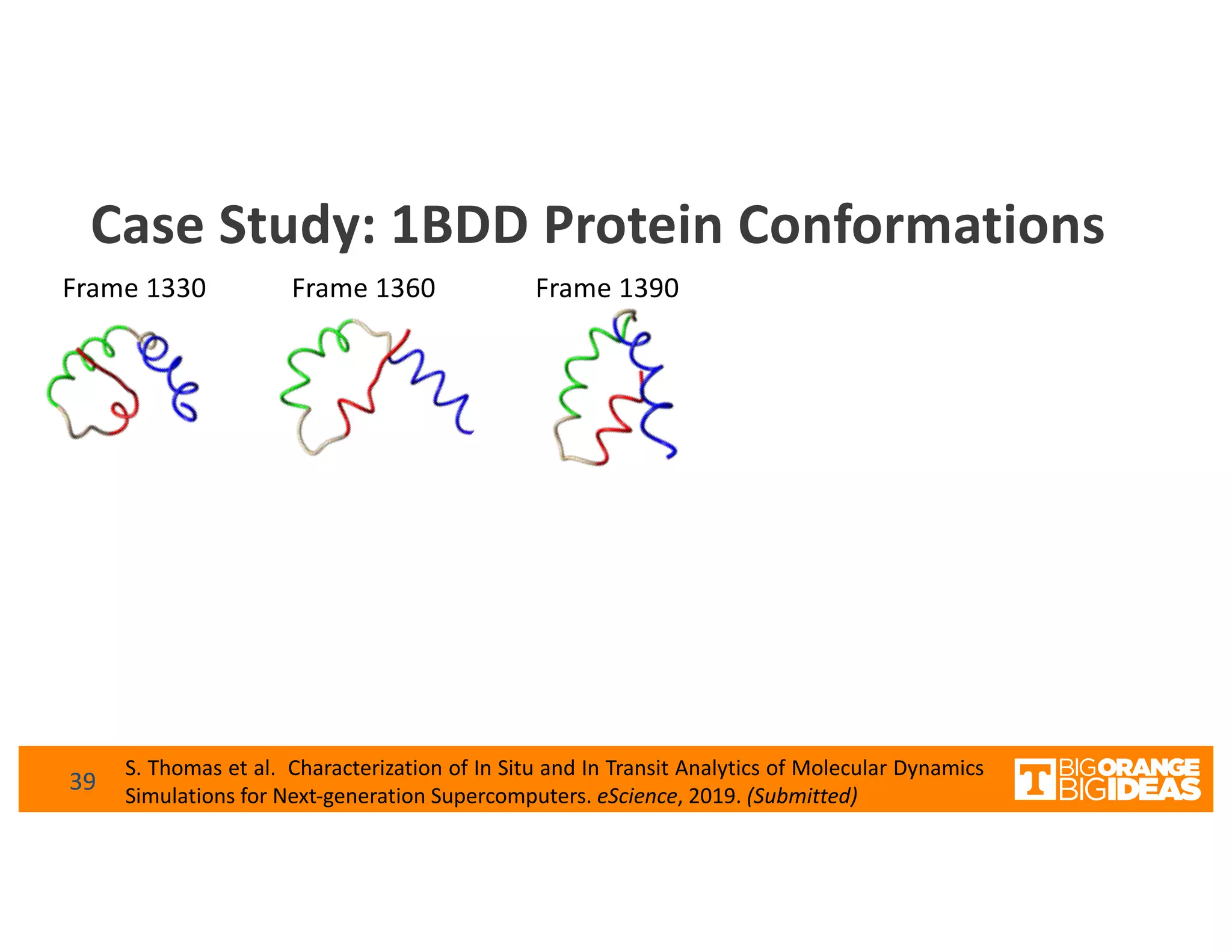
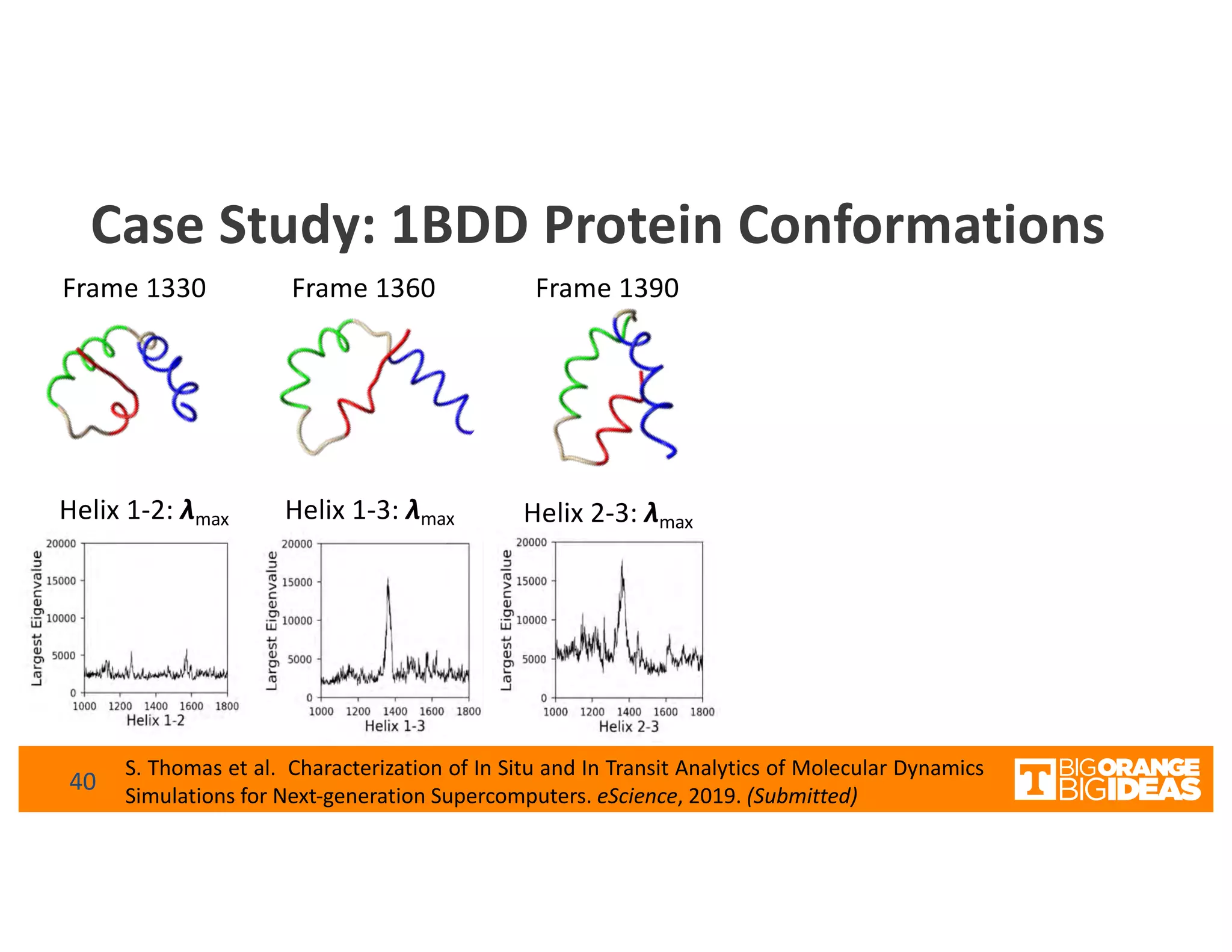
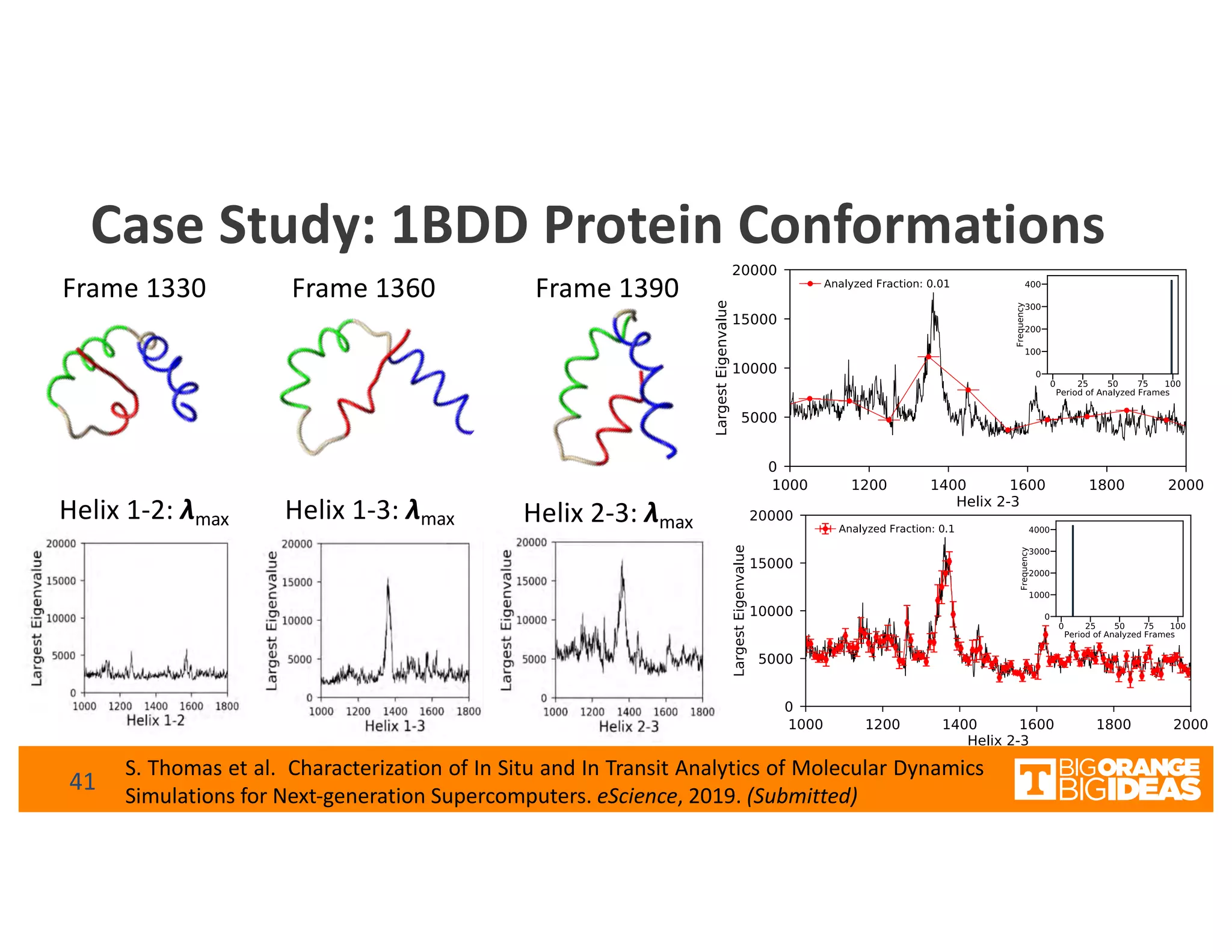
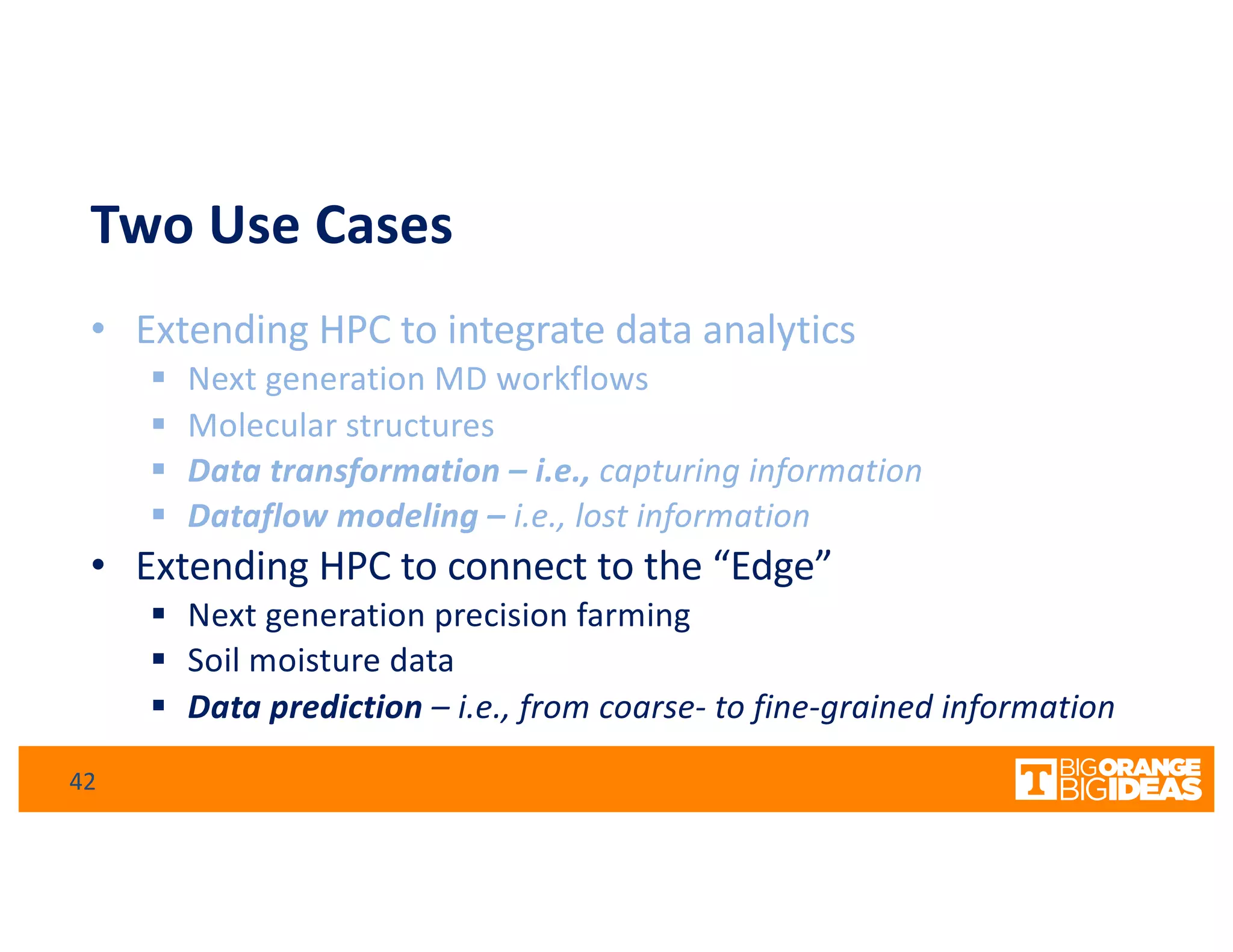
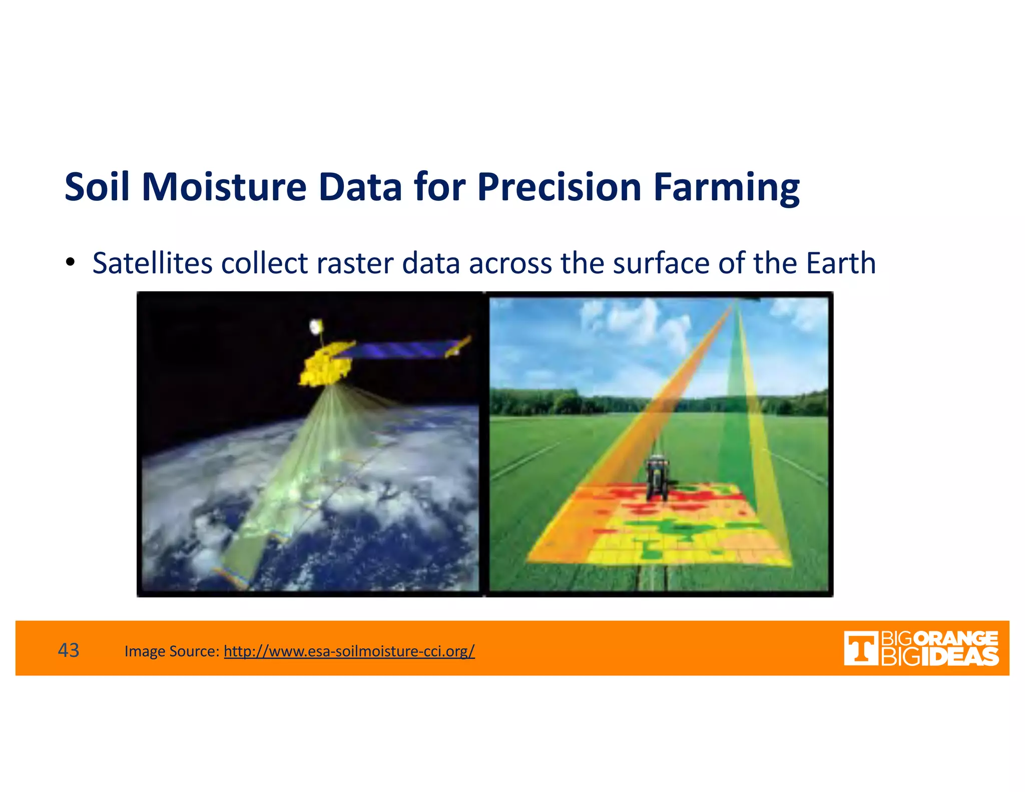
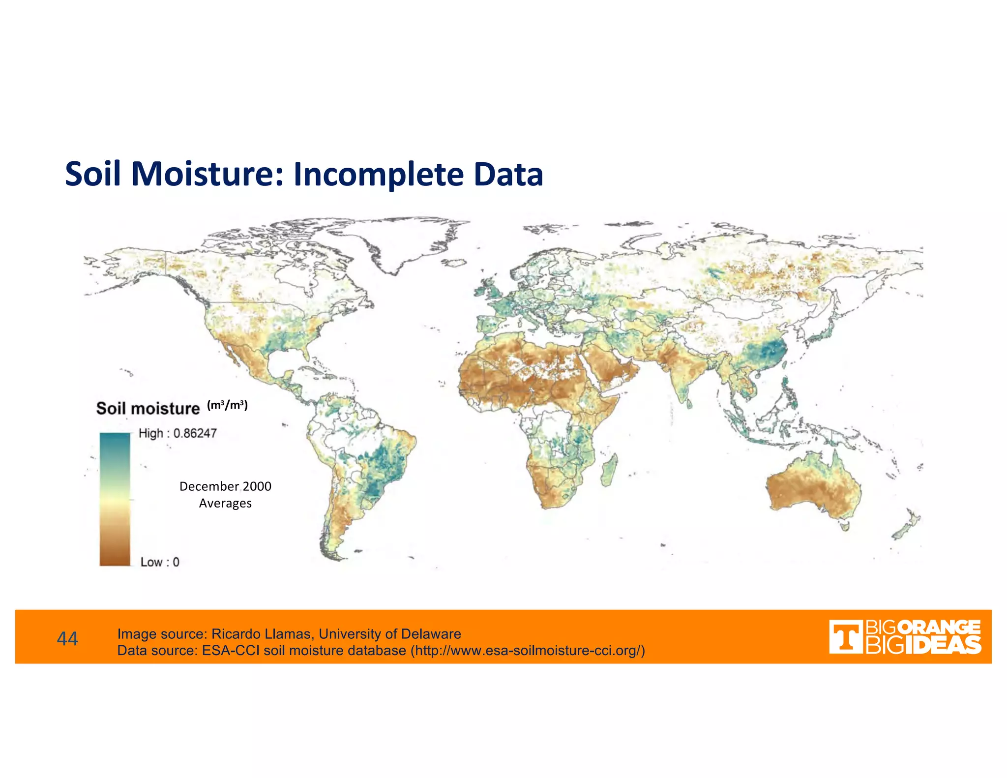
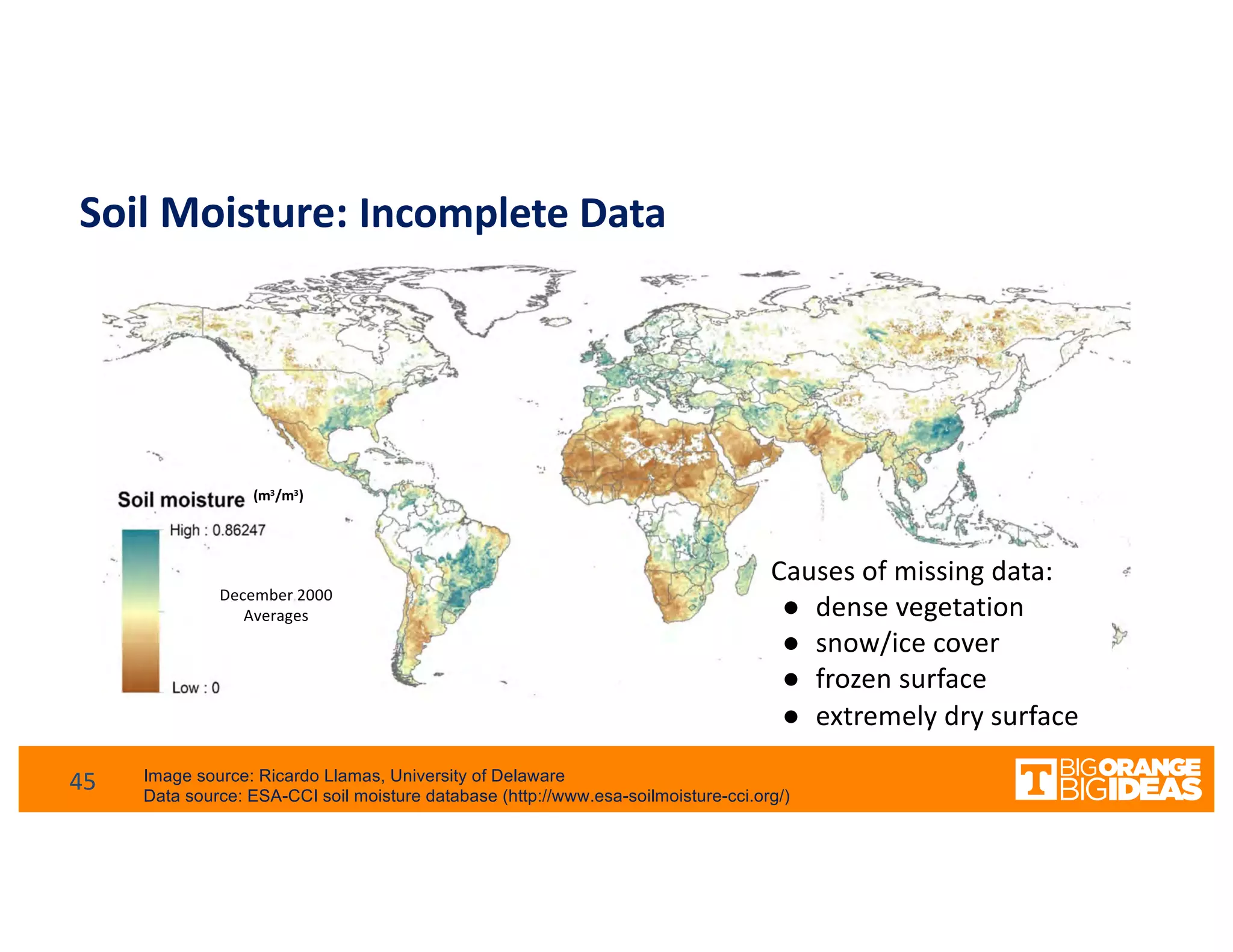
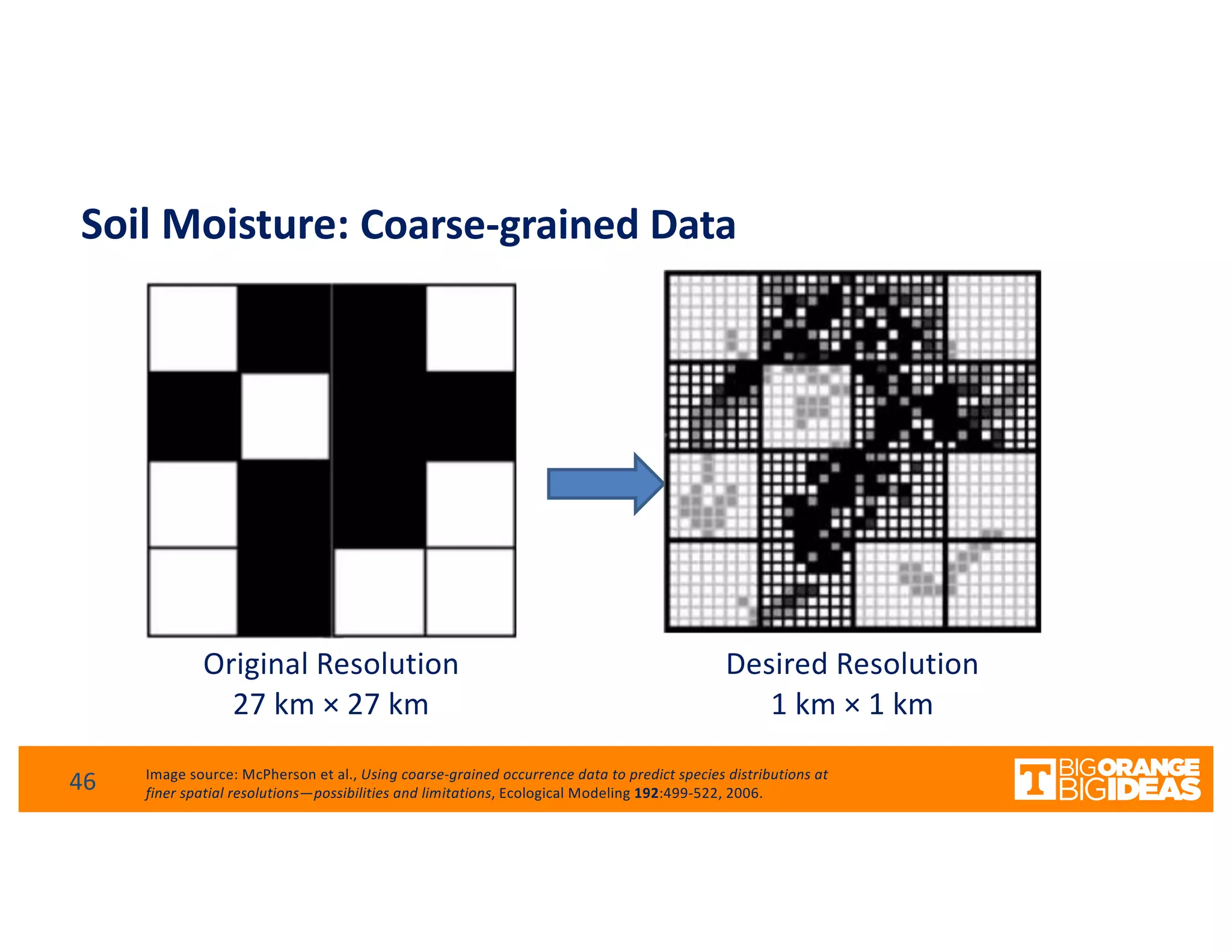
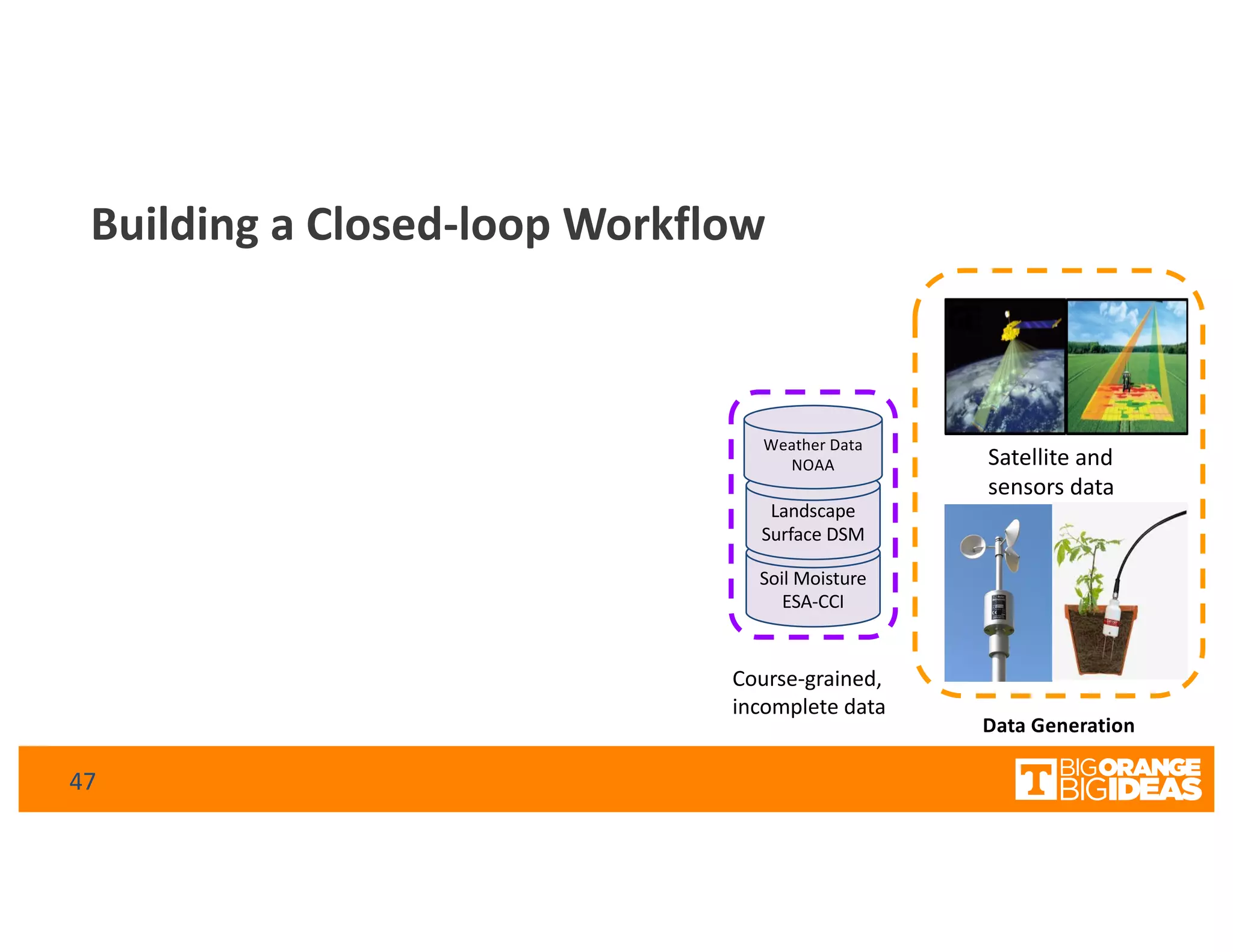
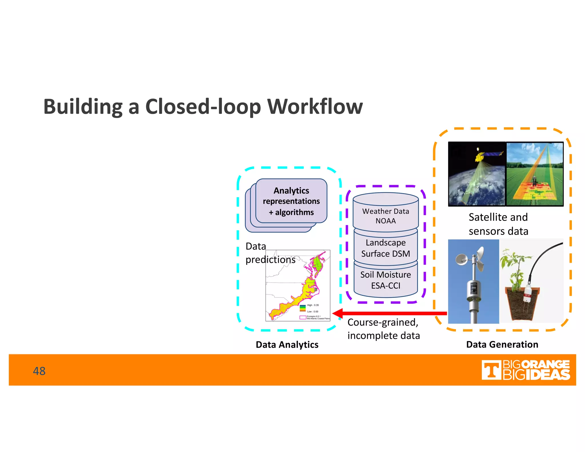
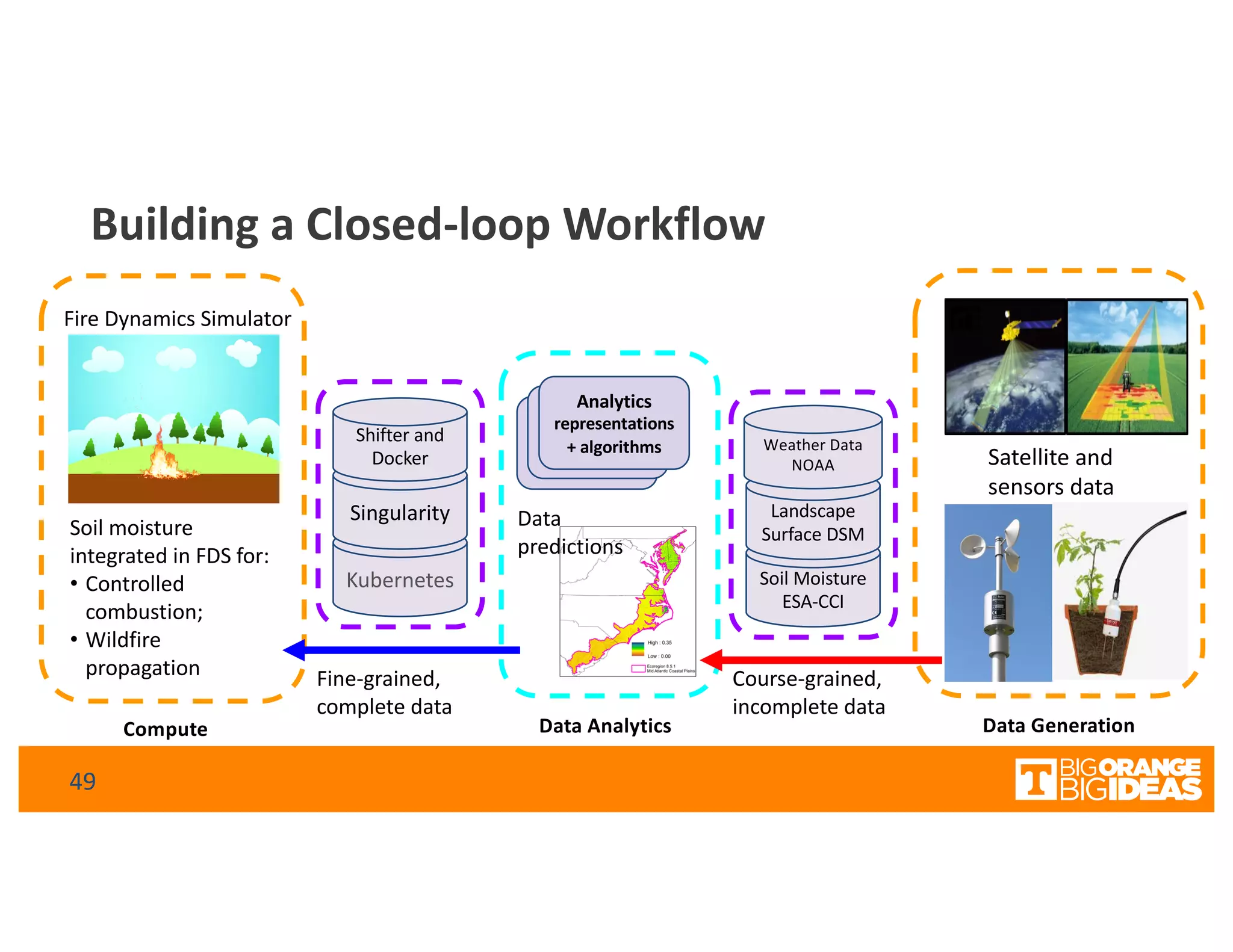
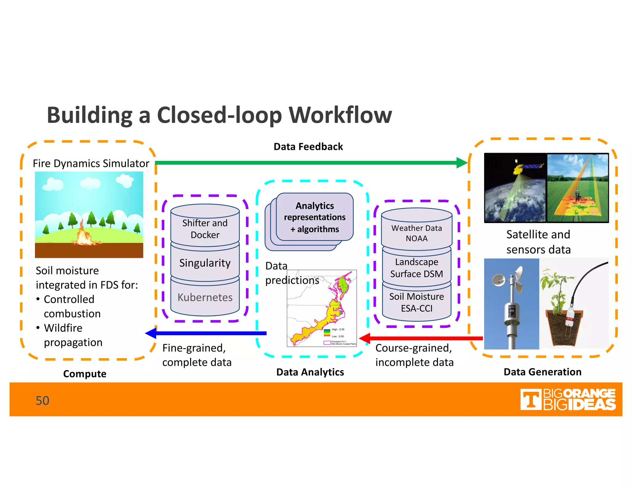
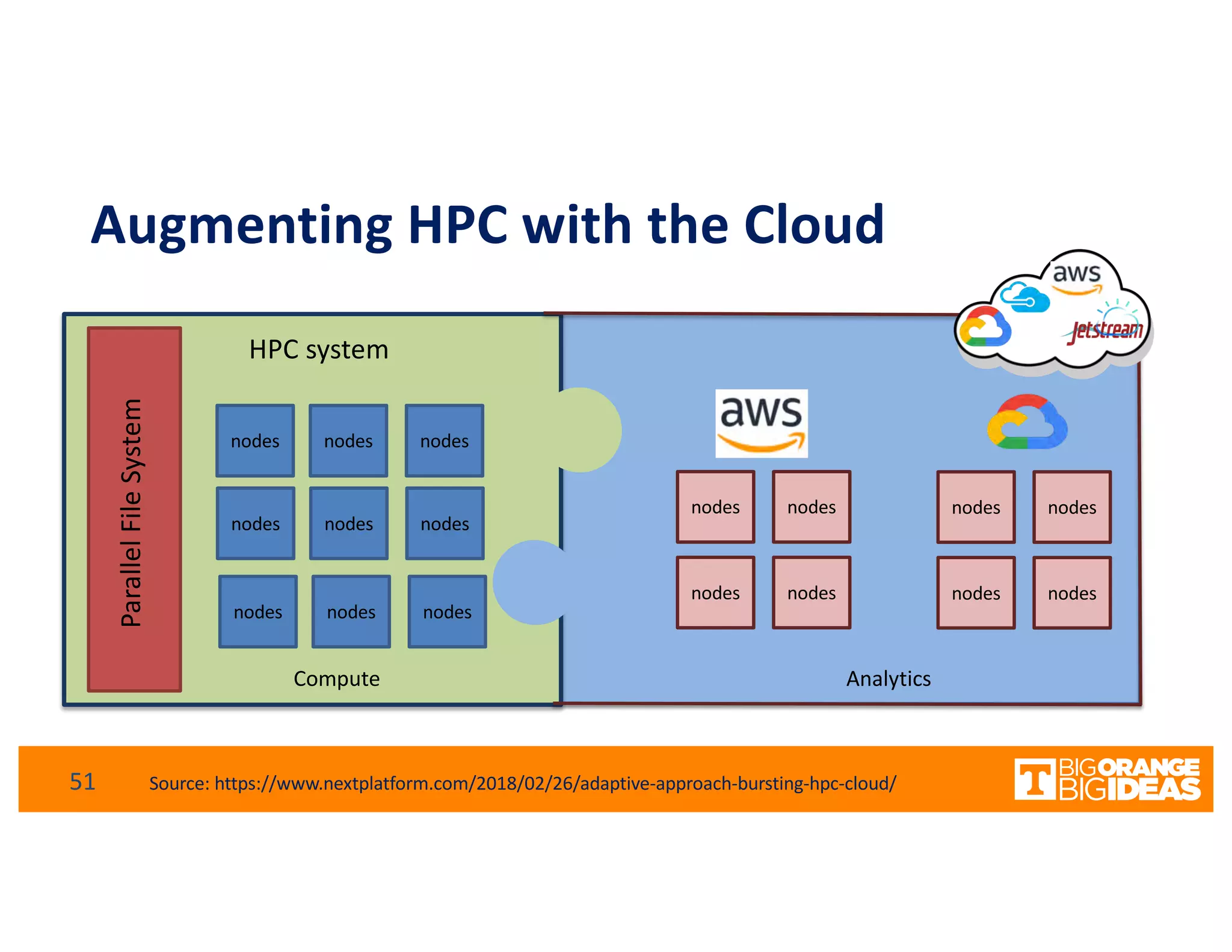

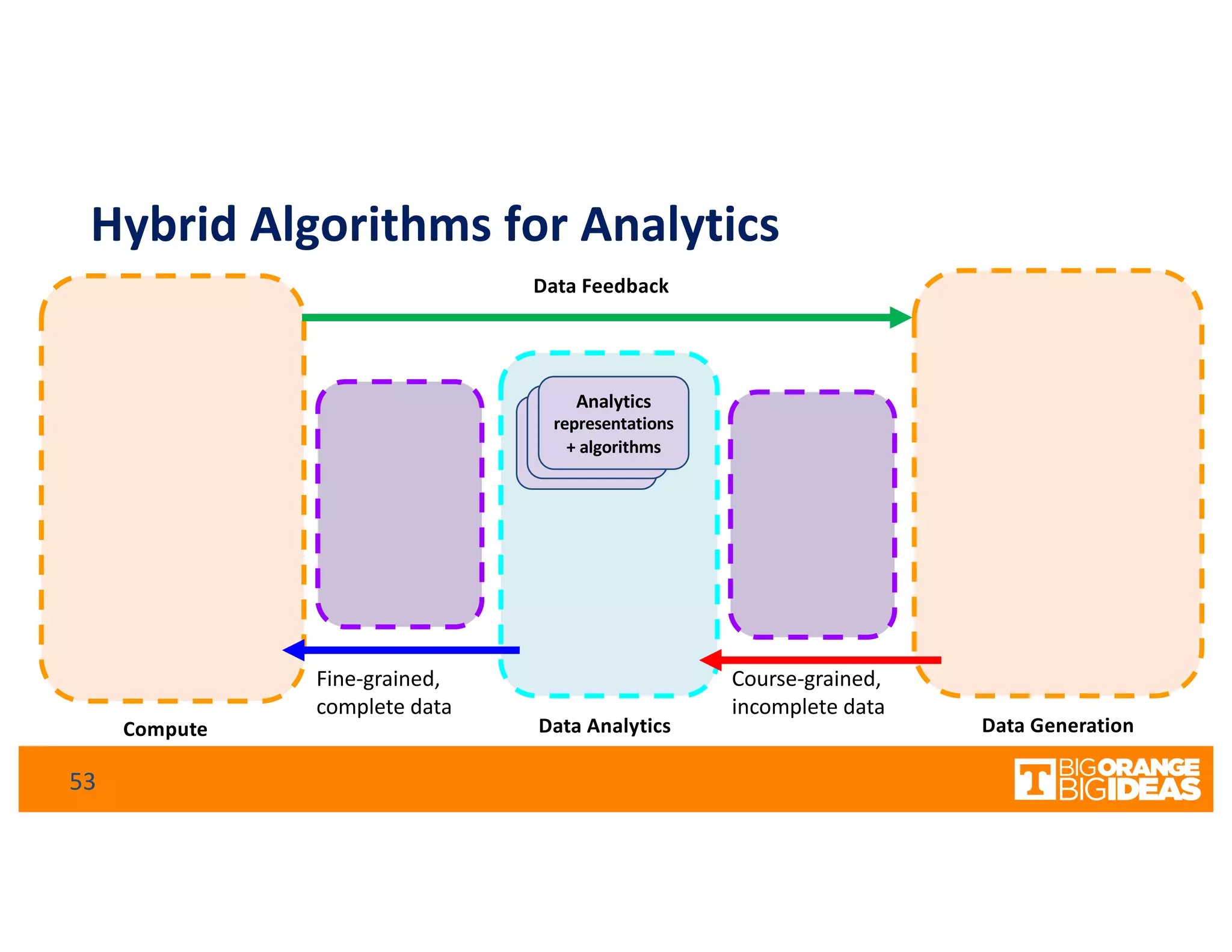
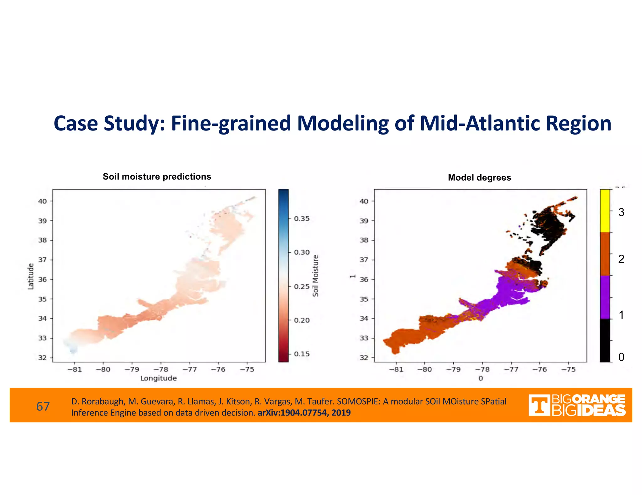
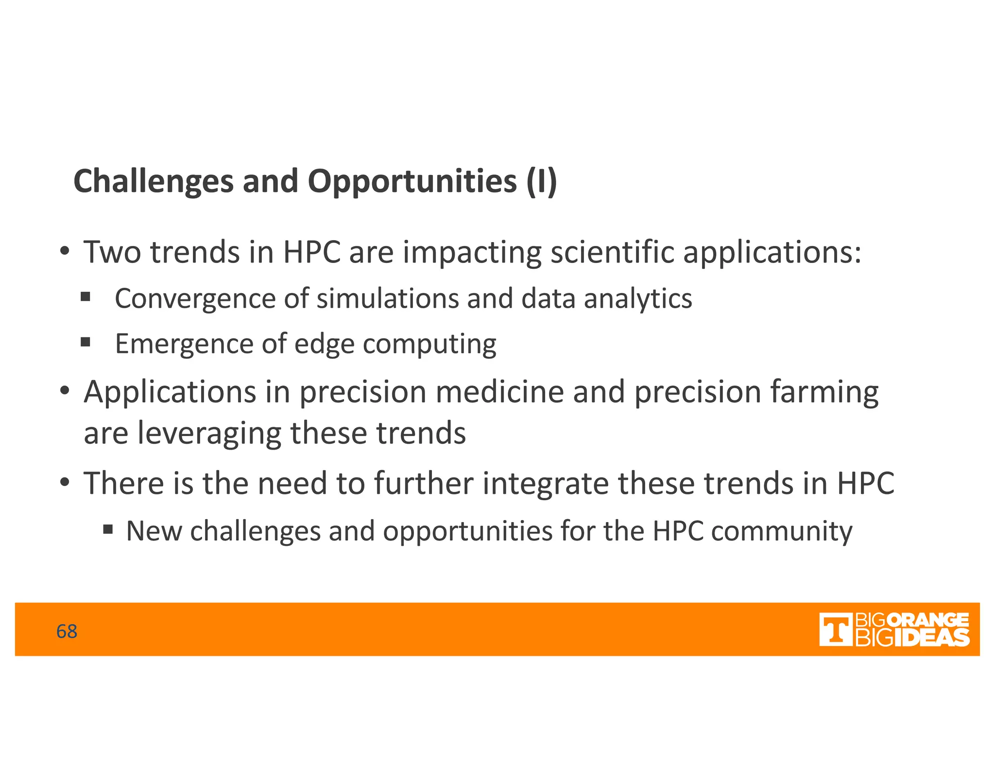
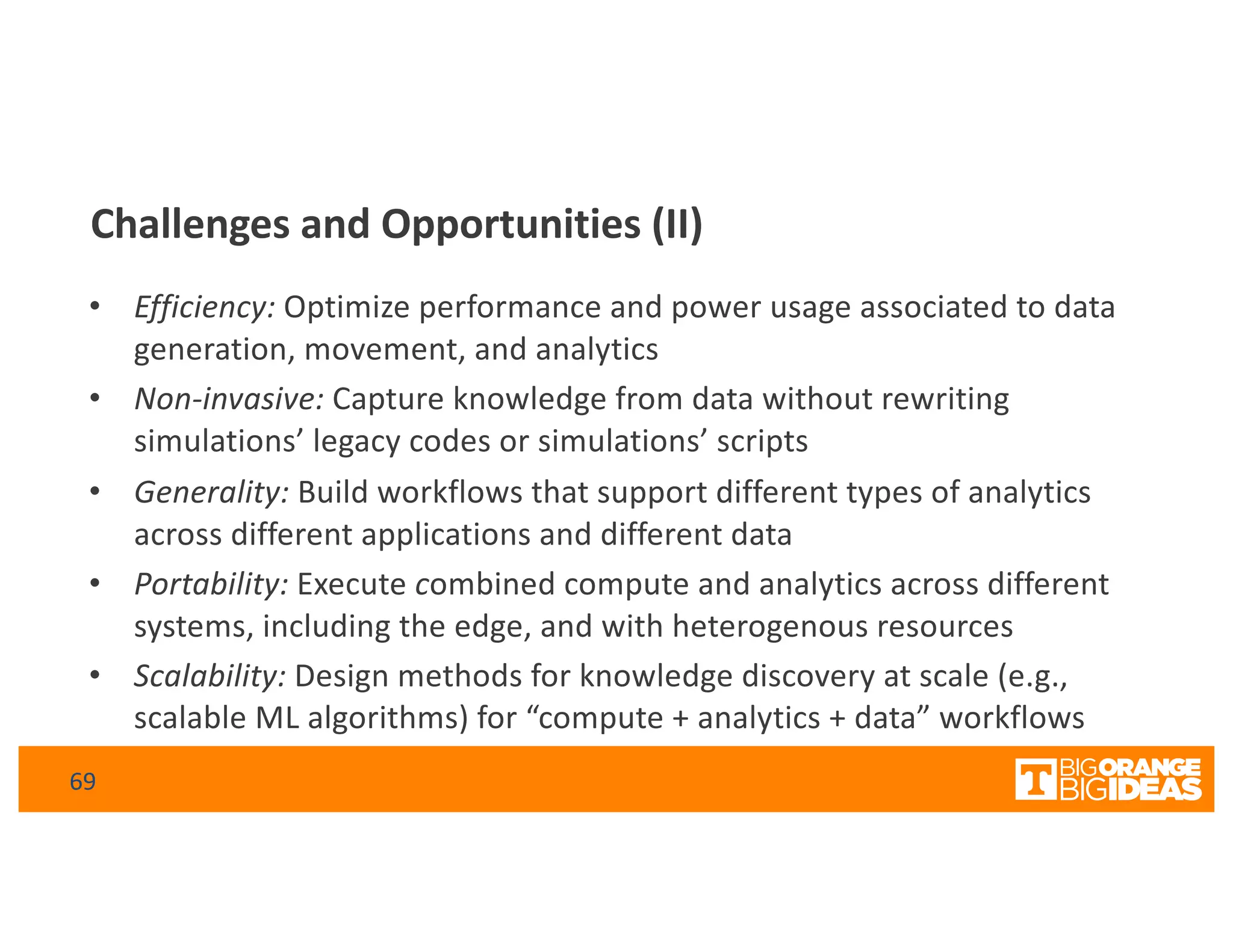


This document discusses extending high-performance computing (HPC) to integrate data analytics and connect to edge computing. It presents two use cases: 1) augmenting molecular dynamics workflows with in situ and in transit analytics to capture protein structural information, and 2) connecting HPC to sensors at the edge for precision farming applications involving soil moisture data prediction. The document outlines approaches for building closed-loop workflows that integrate simulation, data generation, analytics, and data feedback between HPC and edge resources to enable real-time decision making.


![[系列活動] 資料探勘速遊](https://cdn.slidesharecdn.com/ss_thumbnails/0114ycchendmquicktour-170110050658-thumbnail.jpg?width=640&height=640&fit=bounds)