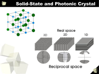
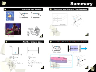
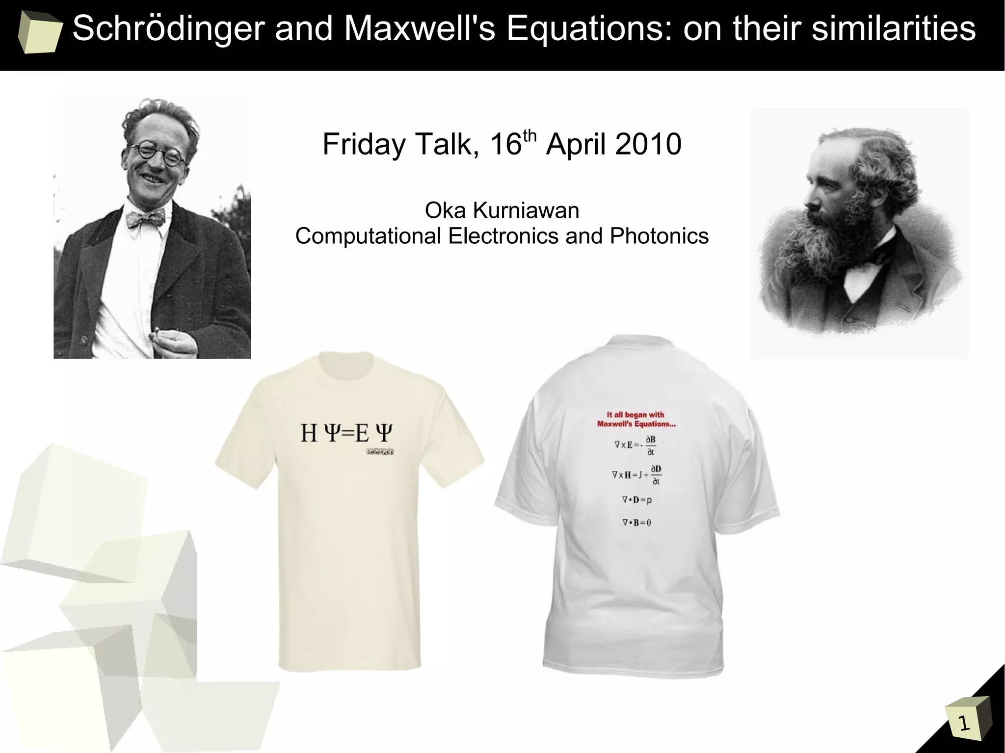
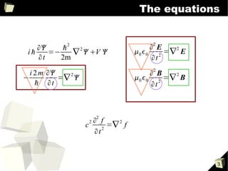
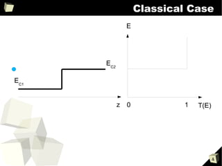
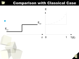
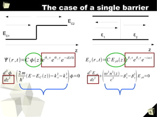
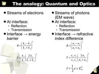
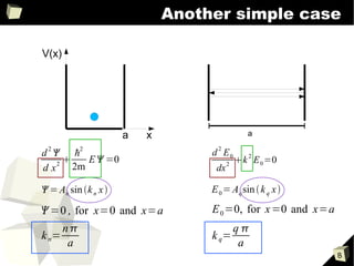
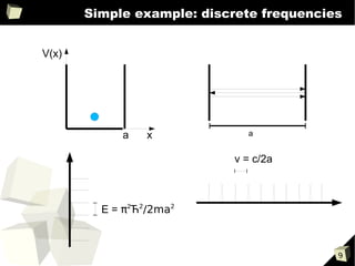
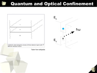
1) Schrödinger's equation for electrons and Maxwell's equations for photons describe wave-like behavior and have similar forms. 2) Both equations can be used to model reflection and transmission of waves at interfaces between different media, analogous to electrons encountering energy barriers or photons encountering changes in refractive index. 3) Simple examples like particles or light in a 1D box show that both systems exhibit quantization of energy levels and discrete frequencies according to the boundary conditions.

1. Schrödinger and Maxwell's Equations: on their similarities
Friday Talk, 16th April 2010
Oka Kurniawan
Computational Electronics and Photonics
1

2. Electron and Photon
E2 E2
ħω ħω
E1 E1
2

3. The equations
2 2
 ℏ 2  E 2
iℏ =−  V  0 0 = E
t 2m t 2
i 2 m  2 B
−
2
=  0 0 2 = 2 B
ℏ t t
2
2 f 2
c 2
= f
t
3

4. Classical Case
E
EC2
EC1
z 0 1 T(E)
4

5. Comparison with Classical Case
E
EC2
EC1
z 0 1 T(E)
5

6. The case of a single barrier
EC2
EC1 ε1 ε2
z z
ik x x ik y y −iEt/ ħ x x y y −i  t
 r ,t =C  z  e e e E y r , t=C E y0  z  e e e
2
   
2
d  2m 2 2 d E y0 2
 n z 
2
2 2
2
 2  E −E C  z −k x −k y =0  − x − y E y0 =0
dz ħ dz 2 c2
6

7. The analogy: Quantum and Optics
■ Streams of electrons ■ Streams of photons
(EM wave)
■ At interface: ■ At interface:
 Reflection  Reflection
 Transmission  Transmission
■ Interface → energy ■ Interface → refractive
barrier index difference
2 2
R=

k 1−k 2
k 1k 2  R=

n1−n2
n1n2 
2 2
T=

k 2 2 k1
k 1 k 1k 2  T=

2 v 2 2 n1
1 v 1 n1n 2 
1 2
I =  v E0
2 7

8. Another simple case
V(x)
a x a
d 2  ħ2 d 2 E0 2
2
 E =0 k E 0 =0
dx 2m dx
2
= An sin k n x  E 0 = Aq sin  k q x 
=0 , for x=0 and x=a E 0 =0, for x =0 and x=a
n q
k n= k q=
a a
8

9. Simple example: discrete frequencies
V(x)
a x a
v = c/2a
E = π2Ћ2/2ma2
9

10. Quantum and Optical Confinement
EC
ħω
EV
Taken from wikipedia
10

11. Laser: Light Amplification by Stimulated Emission of Radiation
E2
ħω ħω
ħω Active medium
E1
Active medium
a
EC
ħω
EV
11

12. Nano Laser
[1] M.T. Hill,et al., “Lasing in metallic-coated nanocavities,”
Nat Photon, vol. 1, Oct. 2007, pp. 589-594.
12

13. References
■ Datta, “Quantum Phenomena,” Modular Series on Solid State Devices, Vol VIII, Addison-
Wesley (1989). page 12-28.
■ Joannopoulus, et al., “Photonic Crystals: Molding the flow of light,” 2nd Ed, Princeton
(2008). page 22 and Appendix A. (E-book download from TWiki)
13

14. Solid-State and Photonic Crystal
14

15. Summary
15