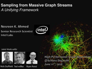
Download as PDF, PPTX


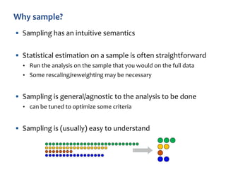
![t=1 t=2
[1, 5] [6, 10]
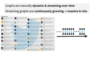
Discrete-time models: represent dynamic network as a sequence
of static snapshot graphs where
User-defined aggregation time-interval
Very coarse representation with
noise/error problems
Difficult to manage at a large scale
Streaming Model](https://image.slidesharecdn.com/dagstuhl-graph18-180717125839/85/Sampling-from-Massive-Graph-Streams-A-Unifying-Framework-6-320.jpg)


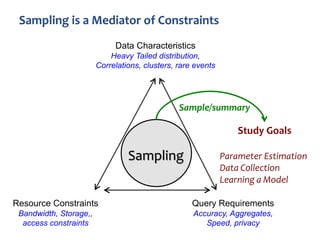

![“Reservoir sampling” described by [Knuth 69, 81]; enhancements
[Vitter 85]
§ Fixed size k uniform sample from arbitrary size N stream in one
pass
§ No need to know stream size in advance
§ Include first k items w.p. 1
§ Include item n > k with probability p(n) = k/n, n > k
— Pick j uniformly from {1,2,…,n}
— If j ≤ k, swap item n into location j in reservoir, discard
replaced item
Easy to prove the uniformity of the sampling method](https://image.slidesharecdn.com/dagstuhl-graph18-180717125839/85/Sampling-from-Massive-Graph-Streams-A-Unifying-Framework-15-320.jpg)
![§ Single-pass algorithms for arbitrary-ordered graph streams
• Streaming-Triangles – [Jha et al. KDD’13]
— Sample edges using reservoir sampling, then sample pairs of incident
edges (wedges), and finally scan for closed wedges (triangles)
• Neighborhood Sampling – [Pavan et al. VLDB’13]
— Sampling vectors of wedge estimators, scan the stream for closed wedges
(triangles)
• TRIEST– [De Stefani et al. KDD’16]
— Uses standard reservoir sampling to maintain the edge sample
• MASCOT– [Lim et al. KDD’15]
— Bernoulli edge sampling with probability p
• Graph Sample & Hold– [Ahmed et al. KDD’14]
— Weighted conditionally independent edge sampling](https://image.slidesharecdn.com/dagstuhl-graph18-180717125839/85/Sampling-from-Massive-Graph-Streams-A-Unifying-Framework-16-320.jpg)


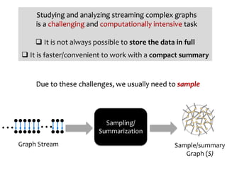
![(1) Challenges for streaming graph analysis
(2) A framework for sampling/summarization of massive
streaming graphs
✓
[Ahmed et al., VLDB 2017], [Ahmed et al., IJCAI 2018]](https://image.slidesharecdn.com/dagstuhl-graph18-180717125839/85/Sampling-from-Massive-Graph-Streams-A-Unifying-Framework-19-320.jpg)
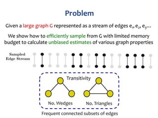
![§ Order sampling a.k.a. bottom-k sample, min-hashing
§ Uniform sampling of stream into reservoir of size k
§ Each arrival n: generate one-time random value rn Î U[0,1]
• rn also known as hash, rank, tag…
§ Store k items with the smallest random tags
§ Each item has same chance of least tag, so still uniform
0.391 0.908 0.291 0.555 0.619 0.273](https://image.slidesharecdn.com/dagstuhl-graph18-180717125839/85/Sampling-from-Massive-Graph-Streams-A-Unifying-Framework-20-320.jpg)

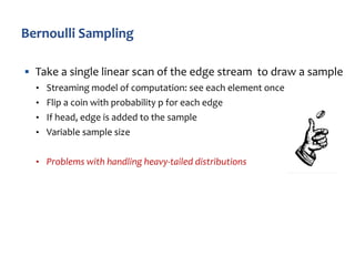
![Input
Graph Priority Sampling Framework
GPS(m)
Output
For each edge k
Generate a random number
u(k) ⇠ Uni(0, 1]
Edge stream
k1, k2, ..., k, ...
Sampled Edge stream ˆK
Stored State m = O(| ˆK|)
Compute edge weight
w(k) = W(k, ˆK)
Compute edge priority
r(k) = w(k)/u(k)
ˆK = ˆK [ {k}](https://image.slidesharecdn.com/dagstuhl-graph18-180717125839/85/Sampling-from-Massive-Graph-Streams-A-Unifying-Framework-22-320.jpg)


![For each edge i,
we construct a sequence of edge estimators ˆSi,t
We achieve unbiasedness by
establishing that the sequence is a Martingale (Theorem 1)
E[ ˆSi,t] = Si,t
ˆSi,t = I(i 2 ˆKt)/min{1, wi/z⇤
}
where ˆSi,t are unbiased estimators of the corresponding edge
ˆKt is the sample at time t
Edge Estimation
[Ahmed et al, VLDB 2017]](https://image.slidesharecdn.com/dagstuhl-graph18-180717125839/85/Sampling-from-Massive-Graph-Streams-A-Unifying-Framework-25-320.jpg)
![For each subgraph J ⇢ [t],
we define the sequence of subgraph estimators as
ˆSJ,t =
Q
i2J
ˆSi,t
E[ ˆSJ,t] = SJ,t
We prove the sequence is a Martingale (Theorem 2)
Subgraph Estimation
[Ahmed et al, VLDB 2017]](https://image.slidesharecdn.com/dagstuhl-graph18-180717125839/85/Sampling-from-Massive-Graph-Streams-A-Unifying-Framework-26-320.jpg)
![Subgraph Counting
For any set J of subgraphs of G,
ˆNt(J ) =
P
J2J :J⇢Kt
ˆSJ,t
is an unbiased estimator of Nt(J ) = |Jt|
(Theorem 2)
[Ahmed et al, VLDB 2017]](https://image.slidesharecdn.com/dagstuhl-graph18-180717125839/85/Sampling-from-Massive-Graph-Streams-A-Unifying-Framework-27-320.jpg)
![§ We provide a cost minimization approach
• inspired by IPPS sampling in i.i.d data [Cohen et al. 2005]
§ By minimizing the conditional variance of the increment
incurred by the arriving edge in
How the ranks ri,t should be distributed in order to minimize
the variance of the unbiased estimator of Nt(J )?
Nt(J )](https://image.slidesharecdn.com/dagstuhl-graph18-180717125839/85/Sampling-from-Massive-Graph-Streams-A-Unifying-Framework-28-320.jpg)


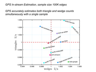
![In-stream Estimation
We define a snapshot as an edge subset J, with a family of
stopping times T such that T = {Tj : j 2 J}
We prove the sequence is a stopped Martingale (Theorem 4)
ˆST
J,t =
Q
j2J
ˆS
Tj
j,t =
Q
j2J
ˆSj,min{Tj ,t}
E[ ˆST
J,t] = SJ,t
[Ahmed et al, VLDB 2017]](https://image.slidesharecdn.com/dagstuhl-graph18-180717125839/85/Sampling-from-Massive-Graph-Streams-A-Unifying-Framework-31-320.jpg)
![q Different weighting schemes lead to
different algorithms
- Uniform weights -> uniform sampling
q Ability to incorporate auxiliary variables
- Using the weight function
q Post-stream estimation
- construction of reference samples
for retrospective queries
q In-stream Estimation
- Maintains the desired query answer
(/variance) and update it accordingly
-> in a sketching fashion
For each edge k
Generate a random number
u(k) ⇠ Uni(0, 1]
Compute edge weight
w(k) = W(k, ˆK)
Compute edge priority
r(k) = w(k)/u(k)](https://image.slidesharecdn.com/dagstuhl-graph18-180717125839/85/Sampling-from-Massive-Graph-Streams-A-Unifying-Framework-33-320.jpg)


![(1) Challenges for streaming graph analysis
(2) A framework for sampling/summarization of massive
streaming graphs
✓
✓
[Ahmed et al., VLDB 2017], [Ahmed et al., IJCAI 2018]](https://image.slidesharecdn.com/dagstuhl-graph18-180717125839/85/Sampling-from-Massive-Graph-Streams-A-Unifying-Framework-44-320.jpg)
![§ Queries Beyond triangles
• Higher-order subgraphs
§ Streaming bipartite network projection
§ Approximate one-mode bipartite graph projection
§ To estimate similarity among one set of the nodes
§ Adaptive sampling
• Adaptive weights vs fixed weight
• Insertion/deletion streams – other dynamics
§ Batch computations, libraries …
To appear [Ahmed et al., IJCAI 2018]
To appear [Ahmed et al., IJCAI 2018]](https://image.slidesharecdn.com/dagstuhl-graph18-180717125839/85/Sampling-from-Massive-Graph-Streams-A-Unifying-Framework-45-320.jpg)

![§ On sampling from massive graph streams. VLDB 2017, [Ahmed et al.]
§ Sampling for Bipartite Network Projection. IJCAI 2018, [Ahmed et al.]
§ A space efficient streaming algorithm for triangle counting using the birthday paradox. KDD 2013, [Jha et. al]
§ Counting and Sampling Triangles from a Graph Stream. VLDB 2013. {Pavan et. al]
§ Efficient Graphlet Counting for Large Networks. ICDM 2015, [Ahmed et al.]
§ Graphlet Decomposition: Framework, Algorithms, and Applications. J. Know. & Info. 2016 [Ahmed et al.]
§ Estimation of Graphlet Counts in Massive Networks. IEEE TNNLS 2018 [Rossi-Zhou-Ahmed]
§ MASCOT: Memory-efficient and Accurate Sampling for Counting Local Triangles in Graph Streams. KDD 2015. [Lim et. al]
§ Network Motifs: Simple Building Blocks of Complex Networks. Science 2002, [Milo et al.]
§ Graph Sample and Hold: A Framework for Big Graph Analytics. KDD 2014 [Ahmed-Duffield-Neville-Kompella]
§ Role Discovery in Networks. IEEE TKDE 2015 [Rossi-Ahmed]
§ Efficient semi-streaming algorithms for local triangle counting in massive graphs. KDD 2008 [Becchetti et al.]
§ Random sampling with a reservoir. ACM Transactions on Mathematical Software (TOMS) 1985. [Vitter]](https://image.slidesharecdn.com/dagstuhl-graph18-180717125839/85/Sampling-from-Massive-Graph-Streams-A-Unifying-Framework-47-320.jpg)

The document discusses advanced techniques for streaming graph analysis, focusing on sampling and unbiased estimation methods to handle massive dynamic graphs. It introduces a priority sampling framework that efficiently estimates various graph properties while addressing challenges such as computational feasibility and memory constraints. The work demonstrates the effectiveness of the proposed methods through real-world applications and empirical results.


![Differential privacy without sensitivity [NIPS2016読み会資料]](https://cdn.slidesharecdn.com/ss_thumbnails/nipsyomi2016slideshare-170122091905-thumbnail.jpg?width=640&height=640&fit=bounds)


![[DSC Europe 25] Dragan Jerosimovic - The Anatomy of a Narrative Simulation.pdf](https://cdn.slidesharecdn.com/ss_thumbnails/vzputuprdqr6zwbrwdcw-1-dragan-jerosimovic-the-anatomy-of-a-narrative-simulation-260114111931-9d04fba2-thumbnail.jpg?width=640&height=640&fit=bounds)


![[DSC Europe 25] Stefan Brankovic - #ResumeIsDead. AI-Powered Interviews and C...](https://cdn.slidesharecdn.com/ss_thumbnails/qnmbsv0xq3uysdrq3sev-2-stefan-brankovic-job-bolt-260114111931-a065aa3d-thumbnail.jpg?width=640&height=640&fit=bounds)


![[DSC Europe 25] Slobodan Dolinic - Smart and Intelligent Green Region.pptx](https://cdn.slidesharecdn.com/ss_thumbnails/0bribinjsp6ghwtvsvor-2-sigre-slobodan-dolinic-260115093812-c9c10e90-thumbnail.jpg?width=640&height=640&fit=bounds)


![[DSC Europe 25] Ivica Milaric - The Future of Gaming and AI Tools.pptx](https://cdn.slidesharecdn.com/ss_thumbnails/tijgzsmgse2kj2y5pzzp-5-ivica-milaric-the-future-of-gaming-x-ai-tools-260114111931-87c2b3ac-thumbnail.jpg?width=640&height=640&fit=bounds)
